Static versus dynamic heterogeneities in the Edwards-Anderson-Ising spin glass
Abstract
We numerically study the aging properties of the dynamical heterogeneities in the Ising spin glass. We find that a phase transition takes place during the aging process. Statics-dynamics correspondence implies that systems of finite size in equilibrium have static heterogeneities that obey Finite-Size Scaling, thus signaling an analogous phase transition in the thermodynamical limit. We compute the critical exponents and the transition point in the equilibrium setting, and use them to show that aging in dynamic heterogeneities can be described by a Finite-Time Scaling Ansatz, with potential implications for experimental work.
pacs:
75.50.Lk, 75.40.Mg, 75.10.NrSpin glasses, fragile molecular glasses, polymers, colloids, and many other materials display a dramatic increase of characteristic times when cooled down to their glass temperature, Cavagna (2009). This is probably due to the collective movements of an increasing number of elements in the system, with a (free) energy barrier growing with the size of the cooperative regions Adam and Gibbs (1965) (the cooperative regions become larger as the temperature gets closer to ). Experimentally, one can get the fingerprints of these movements by observing dynamical heterogeneities Weeks et al. (2000) or non-linear susceptibilities Berthier et al. (2005).
Below , aging appears Vincent et al. (1996). Consider a rapid quench from a high temperature to the working temperature (), where the system is left to equilibrate for time and probed at a later time . One finds that the response functions (e.g., magnetic susceptibility) depend on , with Vincent et al. (1996); Rodriguez et al. (2003); Dupuis et al. (2005). The age of the glass, , remains the relevant time scale even for days.
Dynamical heterogeneities age as well, as found numerically in their characteristic length Jaubert et al. (2007); Belletti et al. (2009). Recent measurements of aging correlation and response functions with space-time resolution Oukris and Israeloff (2009) suggest that will soon be experimentally investigated. Characterizing aging for is our main concern here.
We focus on spin glasses, an easier case for a number of reasons: (i) the sluggish dynamics is known to be due to a thermodynamic phase transition at Gunnarsson et al. (1991); Palassini and Caracciolo (1999); Ballesteros et al. (2000); (ii) the size of the glassy magnetic domains, , is experimentally accessible Joh et al. (1999); Bert et al. (2004) ( lattice spacings at Joh et al. (1999), larger than comparable measurements for structural glasses Berthier et al. (2005)); (iii) , Belletti et al. (2009) suggests that free-energy barriers grow in spin glasses as , rather than with a power law as in fragile glasses; (iv) equilibrium physics is known to rule nonequilibrium dynamics Franz et al. (1998). A quantitative correspondence exists between equilibrium and nonequilibrium spatial correlation functions Belletti et al. (2008); Álvarez Baños et al. (2010) (equilibrium on systems of size matches nonequilibrium at time ). Finally, the Janus dedicated computer Belletti et al. (2006) allows us to simulate nonequilibrium dynamics from picoseconds to a tenth of a second Belletti et al. (2008, 2009), and to compute equilibrium correlation functions on lattices as large as , and temperatures as low as Álvarez Baños et al. (2010).
In this paper we show that a phase transition occurs in the aging dynamic heterogeneities. As time proceeds, when the spin correlation function (see below) becomes smaller than the spin glass order parameter , the length scale of the dynamic heterogeneities diverges in the limit of large . We use the statics-dynamics correspondence to investigate this phase transition in the equilibrium setting, focusing on spatial correlation functions (static heterogeneities). Finite-Size Scaling (FSS) yields an accurate estimate of (something never achieved before for a spin glass) as well as of the relevant critical exponents. Back to nonequilibrium, aging turns out to be amazingly well described by a Finite-Time Scaling Ansatz, with critical parameters taken verbatim from the equilibrium computation.
We consider the Edwards-Anderson model on a cubic lattice of size (volume ), with periodic boundary conditions, at . We use Ising spins, , and binary nearest-neighbor couplings. The average over the quenched disorder, denoted by an overline, is taken after the thermal average . We consider two clones of the system, evolving independently under the same set of coupling constants, and taken at the same time . The replica field is and the spin overlap is its spatial average . See Refs. Álvarez Baños et al. (2010) and Belletti et al. (2009) for full details of our equilibrium and nonequilibrium simulations.
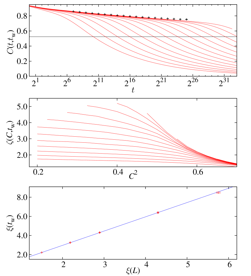
Out of equilibrium, correlation functions depend either on a single time , or on and . Let . The spin correlator, see Fig. 1–top, is
| (1) |
Naive aging is approximatively valid: for finite , decays for long , but the decay slows down with increasing . In fact, there is an enveloping curve with a non-zero limiting value, the order parameter . The lack of a reliable parameterization of precludes a controlled extrapolation of , in contrast with the equilibrium computation shown below.
As for space dependencies, we consider . Using integral estimators Belletti et al. (2008, 2009) we extract the coherence length , the size of regions where the two clones of the system are similar. Yet, to learn about heterogeneities on the dynamics probed at time , at distance , we consider Using an integral estimator Belletti et al. (2009), we extract from the correlation-length , the characteristic length for heterogeneities, displayed in the central panel of Fig. 1. We replace with Cugliandolo and Kurchan (1993), as independent variable. For large , reaches a -independent value, which increases when decreases. On the other hand, for small , grows strongly with . Clearly, something happens when goes through some special value and we intend to exploit the statics-dynamics correspondence to clarify it.
How does all this appear from an equilibrium viewpoint? In the limit of large system size , the probability density function for , , has two Dirac’s delta contributions of equal weight at . Replica Symmetry Breaking (RSB) theory Marinari et al. (2000) predicts that has a support for , while droplet theory expects no support in that region Bray and Moore (1987).
Our approach focuses on the study of equilibrium connected correlation functions Contucci et al. (2009), regarded as a function of the spin overlap . Varying at fixed a phase transition is encountered for . As in Álvarez Baños et al. (2010), our conditional correlation function at fixed , , is obtained as a quotient of the convolutions of and with a Gaussian of width . This combines levels, thus smoothing the comb-like Fernandez et al. (2009).
It has been recently found Belletti et al. (2008); Álvarez Baños et al. (2010) that the equilibrium , computed in a system of size , accurately matches the nonequilibrium if one chooses time such that and time such that (at least at ). It is tempting to assume that the correspondence will become exact in the limit of large and . In Fig. 1–bottom we show an example of this correspondence in the limit .
To proceed with the equilibrium analysis, we observe that tends to for large . In a finite system, one needs to perform a subtraction that complicates the analysis Contucci et al. (2009). We instead consider the Fourier transform at wave vector , , blind to a constant subtraction for . Defining (or permutations), we have
| (2) |
For and , one expects that
| (3) |
(scaling in Fourier space holds only if ). The dots in (3) stand for scaling corrections, subleading in the limit of large (or small ). On the other hand Contucci et al. (2009),
| (4) |
The correlation length diverges when from above, . In principle, is different from the thermal critical exponent at . We note as well the scaling law 111If we add an interaction to the Hamiltonian, (i) the correlation length diverges as ; (ii) , since ; and (iii) (see, e.g., Amit and Martin-Mayor (2005)). Observe that .
| (5) |
The theories for the spin-glass phase differ in the precise form of , but agree that a crossover can be detected in for finite . Indeed, for , while for , see Eqs. (3,4). For large , and the crossover becomes a phase transition. FSS tells us that, see e.g. Amit and Martin-Mayor (2005),
| (6) |
up to scaling corrections. is a scaling function.
We have exploited Eq. (6) in the following non-standard way. We focus on quantities depending on the continuous parameter ():
| (7) |
When is smaller than , vanishes in the large- limit for , while it diverges for . Hence, fixing , the curves for pairs of lattices , will cross at a point , see Fig. 2. To leading order in , the crossing point approaches for large as
| (8) |
Note that the amplitude changes sign at .

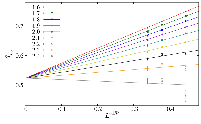
We could use a fit to Eq. (8) in order to obtain the order parameter, but, for a fixed , there are only three crossing points () for three parameters (zero degrees of freedom). Fortunately, one can extract more information from the data by computing the crossings for several values and performing a joint fit, sharing and . Since these additional crossing points are not statistically independent, this procedure requires a proper consideration of the cross-correlations. This can be achieved by computing the fit goodness estimator with the full covariance matrix for the . The number of values considered is a compromise between adding more degrees of freedom and keeping the covariance matrix invertible. We have chosen 9 values of obtaining , reasonable for a fit with degrees of freedom (see Fig. 3). The result is
| (9) |
These numbers are remarkably stable to variations in the set of values. Also, removing the data for (the outliers in Fig. 3) shifts our results by one fifth of the error bars. Note as well that the slope changes sign at . Hence, , in reasonable agreement with Eq. (5).
The value of computed above should be the same as the large- extrapolation of the position of the peak in : a fit , with from (9), yields Álvarez Baños et al. (2010).
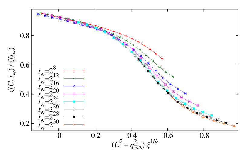
We are finally ready to discuss aging in the dynamic heterogeneities. The statics-dynamics correspondence suggests that it will take the form of a Finite-Time Scaling (FTS) Ansatz, similar to Eq. (6), in which plays the role of . Since it is a length, should have the same scaling dimensions of . Setting short-time corrections aside, Fig. 4 shows indeed that behaves as a function of . FTS also provides a natural explanation for the extremely small exponents found in -extrapolations for 222 In Belletti et al. (2009), we find with . Clearly enough, FTS implies that []. Now, full-aging (as well as empirical evidence Belletti et al. (2009)) suggest that , just as . Therefore ..
In summary, we have studied aging properties in glassy dynamic heterogeneities for the Ising spin glass, characterized through their characteristic length . Aging takes the form of a Finite-Time Scaling Ansatz, which describes the crossover from a regime where is of order one, to a regime where it is of order , the coherence length yielding the size of the glassy magnetic domains. In the limit of an infinite waiting time, the crossover evolves into a phase transition. We have profited from the statics-dynamics correspondence Belletti et al. (2008); Álvarez Baños et al. (2010) to study this phase transition via equilibrium spatial correlation functions, thus obtaining the critical exponents and, for the first time, the spin-glass order parameter. These critical parameters, taken verbatim, describe our nonequilibrium data. For a discussion of the mode-coupling transition in glass-forming liquids in a similar vein see Franz et al. (2010).
Janus was supported by EU FEDER funds (UNZA05-33-003, MEC-DGA, Spain), and developed in collaboration with ETHlab. We were partially supported by MICINN (Spain), through contracts No. TEC2007-64188, FIS2007-60977, FIS2009-12648-C03, by Junta de Extremadura (GRU09038), and by UCM-Banco de Santander. BS and DY were supported by the FPU program (Spain) and SPG by FECYT (Spain).
References
- Cavagna (2009) A. Cavagna, Physics Reports 51, 476 (2009); P. G. Debenedetti and F. H. Stillinger, Nature 410, 259 (2001).
- Adam and Gibbs (1965) G. Adam and J. H. Gibbs, J. Chem. Phys. 43, 139 (1965).
- Weeks et al. (2000) E. R. Weeks, et al., Science 287, 627 (2000).
- Berthier et al. (2005) L. Berthier, et al., Science 310, 1797 (2005).
- Vincent et al. (1996) E. Vincent, et. al in Complex Behavior of Glassy Systems, edited by M. Rubí and C. Pérez-Vicente (Springer, 1997), no. 492 in Lecture Notes in Physics.
- Rodriguez et al. (2003) G. F. Rodriguez, G. G. Kenning, and R. Orbach, Phys. Rev. Lett. 91, 037203 (2003).
- Dupuis et al. (2005) V. Dupuis et al., Pramana J. of Phys. 64, 1109 (2005).
- Jaubert et al. (2007) L. C. Jaubert, C. Chamon, L. F. Cugliandolo, and M. Picco, J. Stat. Mech P05001 (2007).
- Belletti et al. (2009) F. Belletti, et al. (Janus Collaboration), J. Stat. Phys. 135, 1121 (2009).
- Oukris and Israeloff (2009) H. Oukris and N. E. Israeloff, Nature Physics 06, 135 (2010).
- Gunnarsson et al. (1991) K. Gunnarsson, et al., Phys. Rev. B 43, 8199 (1991).
- Palassini and Caracciolo (1999) M. Palassini and S. Caracciolo, Phys. Rev. Lett. 82, 5128 (1999).
- Ballesteros et al. (2000) H. G. Ballesteros, et al., Phys. Rev. B 62, 14237 (2000).
- Joh et al. (1999) Y. G. Joh, et al., Phys. Rev. Lett. 82, 438 (1999).
- Bert et al. (2004) F. Bert, et al., Phys. Rev. Lett. 92, 167203 (2004).
- Franz et al. (1998) S. Franz, M. Mézard, G. Parisi, and L. Peliti, Phys. Rev. Lett. 81, 1758 (1998).
- Belletti et al. (2008) F. Belletti, et al. (Janus Collaboration), Phys. Rev. Lett. 101, 157201 (2008).
- Álvarez Baños et al. (2010) R. Álvarez Baños, et al. (Janus Collaboration), J. Stat. Mech. (2010) P06026.
- Belletti et al. (2006) F. Belletti, et al. (Janus Collaboration), Computing in Science and Engineering 8, 41 (2006).
- Cugliandolo and Kurchan (1993) L. F. Cugliandolo and J. Kurchan, Phys. Rev. Lett. 71, 173 (1993).
- Marinari et al. (2000) E. Marinari, et al., J. Stat. Phys. 98, 973 (2000).
- Bray and Moore (1987) A. J. Bray and M. A. Moore, in Heidelberg Colloquium on Glassy Dynamics, edited by J. L. van Hemmen and I. Morgenstern (Springer, Berlin, 1987), no. 275 in Lecture Notes in Physics.
- Contucci et al. (2009) P. Contucci, et al., Phys. Rev. Lett 103, 017201 (2009).
- Fernandez et al. (2009) L. A. Fernandez, V. Martin-Mayor, and D. Yllanes, Nucl. Phys. B 807, 424 (2009).
- Amit and Martin-Mayor (2005) D. J. Amit and V. Martin-Mayor, Field Theory, the Renormalization Group and Critical Phenomena (World Scientific, Singapore, 2005), 3rd ed.
- Franz et al. (2010) S. Franz, G. Parisi, F. Ricci-Tersenghi, and T. Rizzo (2010), eprint arXiv:1001.1746.