The Jefferson Lab Hall A Collaboration
Exclusive Neutral Pion Electroproduction in the Deeply Virtual Regime
Abstract
We present measurements of the cross section extracted at two values of four-momentum transfer and at Jefferson Lab Hall A. The kinematic range allows one to study the evolution of the extracted cross section as a function of and . Results are confronted with Regge-inspired calculations and GPD predictions. An intepretation of our data within the framework of semi-inclusive deep inelastic scattering is also discussed.
pacs:
13.60.Hb, 13.60.Le, 13.87.Fh, 14.20.Dh, 25.30.RwI Introduction
The past decade has shown a strong evolution of the study of hadron structure through exclusive processes, allowing access to the three-dimensional structure of hadrons.
Exclusive processes include deeply virtual Compton scattering (DVCS) and deeply virtual meson production (DVMP).
This document focuses on the latter, and more precisely on neutral pion production.
We present measurements of the differential cross section for the forward exclusive electroproduction reaction , through virtual photoabsorption.
A diagram of this process, including definitions of the kinematic variables, is presented in Figure 1.
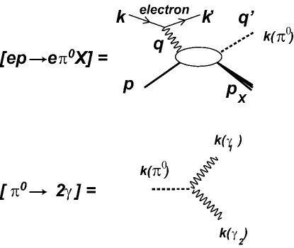
Results will be presented for four kinematics. Two of them are defined by the same value of and are called Kin2 (at ) and Kin3 (at ) The two remaining ones are defined by the same value of and are called Kin2 (at ) and Kin3 (at ).
The behavior of the cross section will be compared to different models that are available to describe electroproduction, including the Regge model and the generalized parton distribution (GPD) framework.
Forward photo-production at asymptotically high energies can be described by the Regge theory, which exploits the analytic properties of the scattering amplitude in the limit Goldstein and Owens (1973). Previous analyses have applied Regge phenomenology to exclusive photo- and electro-production in the kinematic range presented here Guidal et al. (1997a, b). Recent computations with Regge-inspired models exist for our kinematics. These models include , , and meson exchange as well as rescattering. Among these, there is the -channel meson-exchange (TME) model by Laget et al. A brief description of this model has been given in De Masi et al. (2008), and it is described extensively in Laget (2007, 2011). Recent JLab Hall C experiments studying the dependence of charged-pion electroproduction with a longitudinal-transverse separation were analyzed using the TME formalism Horn et al. (2008). Another Regge-inspired computation by Ahmad, Goldstein and Liuti Ahmad et al. (2009) is available for our kinematics.
In the Bjorken limit , and at fixed , the scattering amplitude is dominated by the leading order (or leading twist) amplitude of GPDs and the pion distribution amplitude (DA) Collins et al. (1997); Goeke et al. (2001); Vanderhaeghen et al. (1999). The GPDs are light-cone matrix elements of non-local bilinear quark and gluon operators Mueller et al. (1994); Ji (1997); Radyushkin (1997), unifying the elastic electroweak form factors with the forward parton distributions of deep-inelastic lepton scattering. Cross section predictions within the GPD framework exist for the longitudinal cross section Goeke et al. (2001); Vanderhaeghen et al. (1999). With the definitions of Collins et al. (1997); Goeke et al. (2001); Vanderhaeghen et al. (1999), the cross sections are predicted to scale as and . Thus at sufficiently high , will dominate over . Beam spin asymmetries for forward exclusive electroproduction have been measured for De Masi et al. (2008). We performed measurements at two values at fixed in order to test these predictions of dependence. An interpretation of exclusive data with semi-inclusive mechanisms also exists to explain transverse cross sections of hard exclusive charged-pion electroproduction Kaskulov et al. (2008).
In the second section details of the experiment are presented, while the third section is devoted to the calibration of the calorimeter. The formalism of electroproduction by Drechsel and Tiator Drechsel and Tiator (1992) is presented in the fourth section with a special emphasis on the expressions for the hadronic tensors. The fifth section is devoted to the extraction of the cross sections and the sixth and seventh sections to the radiative corrections and the evaluation of the systematic errors. Finally, our results are presented in Sec. VIII, with a discussion and conclusions in Secs. IX and X, respectively.
II Experiment
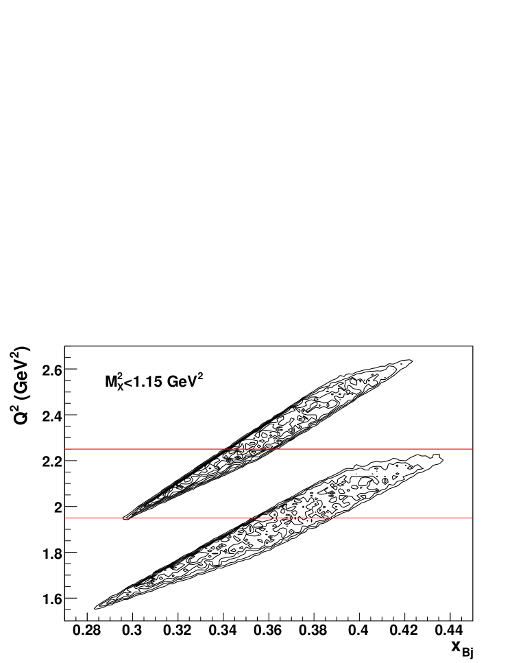
The present data were acquired as part of Jefferson Lab Hall A experiment E00-110 Bertin et al. (2000). Additional details about the experimental configuration, calibrations, and analysis can be found in Muñoz Camacho (2005); Munoz Camacho et al. (2006). This paper reports on the analysis of the triple coincidence events. A 5.75 GeV electron beam was incident on a 15 cm liquid hydrogen target, for a typical luminosity of . Electrons were detected in a high resolution spectrometer (HRS). Photons were detected in a 132 element calorimeter, each of the elements measuring . The high resolution allows one to accurately define (1) the virtual photon, having the kinematics centered at a fixed and two values of and , as shown in Figure 2 and (2) the real photon momentum unit vector, thanks to the vertex resolution of the HRS, and the position resolution of the electromagnetic calorimeter.
The validation threshold for the data acquisition trigger was set to about 1 GeV for each photon cluster. For the exclusive events, the minimum distance between the centroids of the two clusters that guarantees separation is about 10 cm. This is achieved by the minimal opening angle and the distance from the center of the target to the calorimeter front face cm. The achieved coincidence resolving time between the scattered electron and either photon cluster is 0.6 ns, rms.
Figure 2 shows the distribution of events in the [, ] plane, for missing mass squared . The analysis relies only on two specific qualities of the experiment:
-
i
Thanks to the resolution of the spectrometer and the calorimeter, one can use the missing-mass squared to ensure exclusivity. The exclusive sample is selected by putting a cut on the missing-mass squared at the proton plus the pion mass squared.
-
ii
For exclusive events, the reconstruction of the invariant momentum transfer and relies on the positions of the reconstructed photons, of which the resolution is better than that of the energy. From this, a resolution in better than that in the energy is obtained. All data are presented as a function of , which is directly linked to the angle of the pion production relative to the virtual photon direction in the center of mass : .
In the reaction, there are six four-vectors, equivalent to 24 independent kinematic variables. The measured four-vectors , , and , and four-momentum conservation, reduce the number of independent variables to eight. The measurement of the two directional vectors and from the target vertex (reconstructed by the HRS) to the two cluster positions in the calorimeter provides four more kinematic constraints. Finally, the hypothesis that the observed calorimeter showers are due to photons () provides two more kinematic constraints. The remaining two unknowns, which we express as and , are determined by the previous constraints plus the energy of the two photons. Figure 3 displays the distribution of the events in the [, ] plane, for Kin3.
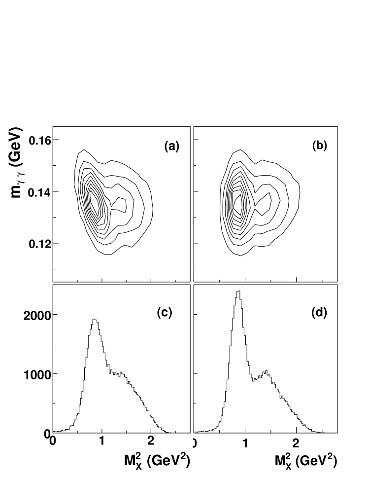
The upper left panel of this figure shows a clear correlation between the two variables in the exclusive region (). This is a consequence of resolution fluctuations in the energies and of the two photons issued from a , which correlate fluctuations in and . The missing mass in the right-hand panels is obtained by an empirical adjustment:
| (1) |
with .
This transformation produces a noticeable improvement in the distribution (lower right panel of Figure 3).
III Calibration
We performed elastic calibrations at the beginning, middle, and end of the experiment Mazouz and Voutier (2005). The calorimeter was retracted to a position at 5.5 m from the target, in order to optimize the electron coverage in the calorimeter with the proton acceptance of the HRS. These data were used for the block calibration. After calibration the calorimeter energy resolution was observed to be 2.4% at 4.2 GeV with a position resolution of 2 mm at 110 cm from the target. The elastic data also provided a consistency check on the efficiency of the detectors and all associated electronics from the observation that the elastic cross section agreed with the Kelly form-factor parametrization Kelly (2004) at the 1.1% level. During the experiment, the light output from the blocks decreased by up to 20%, strongly correlated with the distance of the blocks from the beam line. We attribute this to radiation damage of the blocks. In addition, seven blocks, at random positions, showed much higher radiation damage. One explanation could be a poorer crystal quality of those crystals. We adjusted the calibration of each block, assuming an independent linear dose versus attenuation curve. In addition to radiation damage, each crystal received a pileup of low-energy photons in random coincidence, resulting in a degradation of the energy resolution, and in a shift in the calibration as a function of its distance to the beam line. This effect was taken into account through successive steps:
-
i
For each block the position of the reconstructed missing-mass squared peak was centered at through an energy calibration of the experimental data.
-
ii
A geant simulation generated a sharper resolution in missing mass than the experimental data for each calorimeter block. For each block the energy of the simulation was calibrated together with a simultaneous energy smearing, in order to center the reconstructed missing-mass peak position at , and to equate the resolution of the simulation to that of the experimental data.
These calibrations are explained in the following paragraphs.
We consider only the 90 blocks of the inner calorimeter (see Figure 4 for the labeling), indexed by .
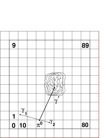
We will assume that the energy of the photon is driven by the block where the shower makes the largest energy deposit. The 90 distributions of missing-mass squared are built with all events involving block . Note that for each event , the reconstructed missing-mass squared appears in two distributions. To compare these distributions, two estimators are constructed: the mean and the sigma of a Gaussian fitted to these distributions, over a limited range (). The calorimeter is calibrated using
| (2) |
with . Neglecting the term compared to between the parentheses, we obtain an energy correction:
| (3) |
We recall here that each event involves two blocks. The reconstructed missing mass of one block is then influenced by contributions from all other blocks. Because of this, several iterations are necessary. Then, the missing-mass distribution of each block for simulated events is adjusted to get the same missing-mass position and resolution as the experimental missing-mass distribution. The missing-mass cut applied to ensure exclusivity is the same for simulation and data, and if the resolution is better for simulation, applying such a cut will remove more experimental events than simulation particularly near the beam where the noise degrades the experimental resolution. This gives a spurious contribution to the term which has to be removed by smearing the simulation resolution. To this purpose, the momentum of each event at the iteration contributing to the distribution of the block is changed from to with a sampling from a Gaussian distribution:
| (4) |
where
| (5) | |||
| (6) |
and is given by equation (3), except we put in this case. The factor 2 in the denominator of is used to ensure a smooth convergence.
| (GeV) | (GeV) | |
| Kin3 | ||
| Data | 0.00081 | 0.0088 |
| Simulation | +0.00072 | 0.0089 |
| Kin2 | ||
| Data | 0.00017 | 0.0079 |
| Simulation | +0.00191 | 0.0085 |
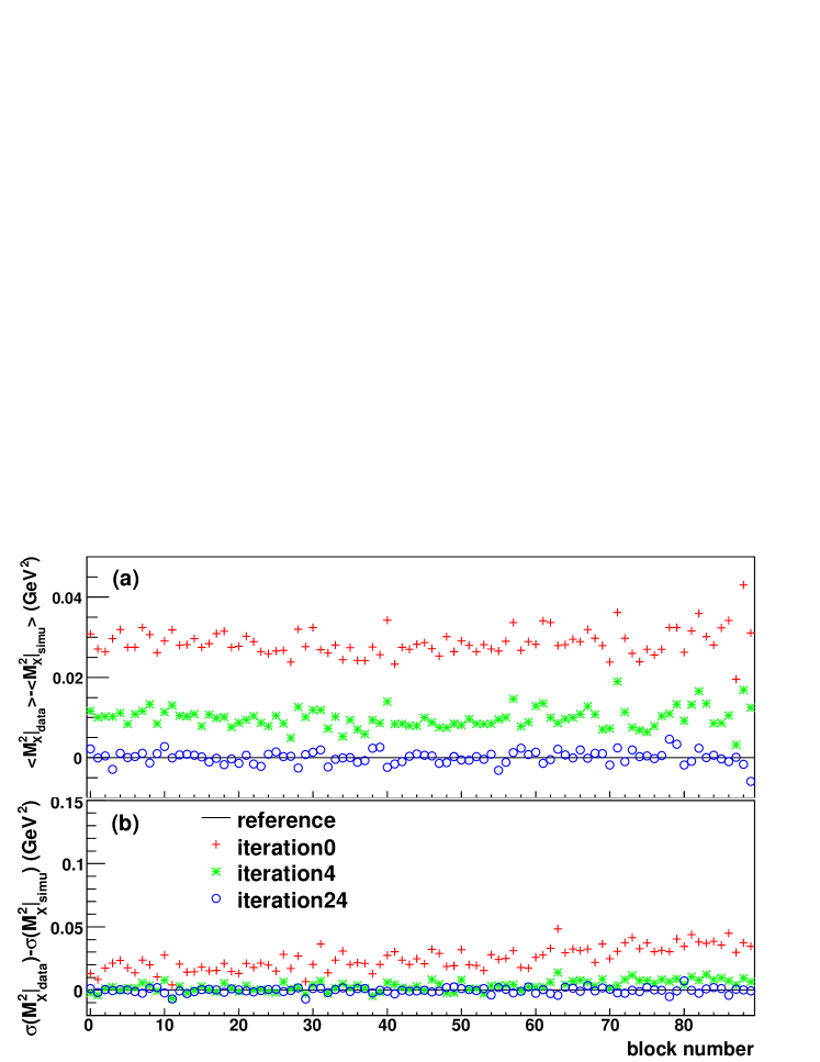
The results of these iterations are shown in Figure 5. Figure 6 and Table 1 illustrate the quality of the final calibration adjustments. The calibration of the missing-mass squared was cross-checked by comparing the invariant-mass distribution of both photons in each event. Table 1 lists the mean values of these distributions with respect to the pion mass, and their resolution. The agreement of the calibration with the data is at the 1.9 MeV level, while the widths of these distributions agree to better than 1 MeV.
IV Cross-section analysis
In order to extract the differential cross section, it is advantageous to incorporate all model-independent kinematic dependences of the differential cross section into the experimental simulation. To this end, we express the differential cross section in terms of structure functions as described in the paper of Drechsel and Tiator Drechsel and Tiator (1992) directly related to bilinear combinations of the Chew-Goldberger-Low-Nambu (CGLN) helicity amplitudes Chew et al. (1957). We define the differential phase-space elements and and the equivalent real photon energy in the c.m. frame . Here with and the norms of , in the center-of-mass frame. All these quantities are defined using the convention of Drechsel and Tiator Drechsel and Tiator (1992): axis along the virtual photon, orthogonal to the leptonic plane, and .
To lowest order in the fine-structure constant , the differential cross section for an electron of helicity is
| (7) |
| (8) |
with and and the energies of the incident and scattered electron, respectively. The virtual photo-absorption cross section is expanded as
| (9) |
where is the c.m. virtual photon three-momentum, is the degree of linear polarization of the virtual photons, and . The response functions are defined as functions of the usual hadronic tensor :
| (10) | |||
| (11) | |||
| (12) | |||
| (13) | |||
| (14) |
The interference terms and have a leading dependence, and the linear polarization interference term has a leading dependence. For this reason, we define reduced structure functions , which remove this phase-space dependence, which are directly related to bilinear combinations of the CGLN helicity amplitudes Chew et al. (1957):
| (15) |
| (16) |
| (17) |
| (18) |
Since our kinematics cover a wide range in as well as in , we also have to include the and the dependence of the hadronic tensor . We perform a preliminary extraction of the cross section on the kinematic points Kin2 and Kin3 (respectively Kin2 and Kin3) to get an estimate of the (respectively, ) dependence of the hadronic tensor. The extracted and dependences are then introduced explicitly in the formalism to perform a second “definitive” extraction. The dependence is modeled in the form and . With the first iteration, the cross sections changed by , but with a second iteration the cross sections changed by only .
The results will be presented as four separated cross sections following the usual decomposition found in the literature:
| (19) |
V Extraction
We define a compact notation that summarizes Eq. (9) in the form
| (20) |
with containing all the kinematic dependence, and summarizing all variables , considered at the vertex. reflects the fact that we used only one incident energy and consequently, we were not able to disentangle and . This notation will be convenient to use for the presentation of the extraction process.
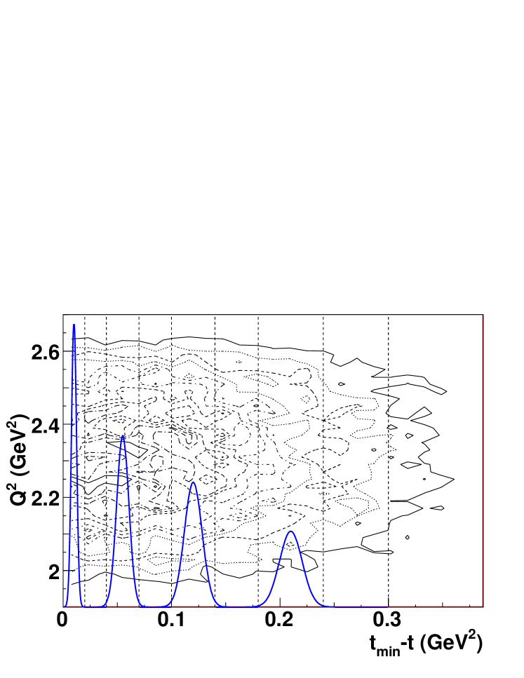
The experimental data used for the analysis have the kinematical coverage shown in Figure 2. The analysis includes a complete simulation of the resolution and acceptance of the HRS, the external and internal radiative effects on the incident and scattered electron, and a geant based simulation of the acceptance and response of the array. Simulation events are generated uniformly in the target vertex along the beam line, and uniformly in a phase space . This results in well defined values of in each bin. The bins are the same in the generation and experimental phase spaces, but resolution and radiative effects can cause the migration of events from one bin to one of its neighbors (Figure 7). Rather than extracting average cross sections in the experimental bins, we use the simulation and the theoretical form of Eq. (20) to directly extract differential cross sections from the experimental yields.
We divide the acceptance into 24 equal bins in and 8 bins in for both the helicity dependent and independent parts of the cross section. A bin in the kinematic variables reconstructed by the detector is defined by the limits , , etc. The statistics in a bin are determined by the physical cross section at the vertex convoluted with the detector response:
where summarizes the reaction vertex variables, summarizes the reaction vertex variables as reconstructed in the detector, summarizes the range of integration for bin , summarizes the range of integration for all bins , is the integrated luminosity, and is the probability distribution for an event originating at the vertex with kinematics to be reconstructed by the detector with vertex kinematics . This expresses the effects of detector resolution, internal and external radiation, detector efficiency, and anything else that could migrate events from vertex kinematics to the detector kinematics . For the analysis and simulation, the integral is split into a sum over the bins in the kinematic variables at the reaction vertex:
Because the functions contain the main part of the dependence on the variables at the vertex, the quantity in a bin will be assimilated to its average in this bin. Then, the last equation can be summarized in a vector notation:
| (21) |
with
| (22) |
We then replace the integration by a summation over the simulated events :
| (23) |
where the sum is over events originating in vertex bin and reconstructed in bin . is the number of events generated in the simulation and is the total phase-space factor. The matrices are constructed from simulation events, summed over all events within cuts. We define with () the number of counts within cuts with positive (negative) electron helicity. The cuts are the same for simulation and data (Table 2). The cuts and the corrections are summarized in Tables 2 and 3, respectively.
| Spectrometer cuts |
| 6.0 cm +7.5 cm |
| 3.5 cm |
| (Horizontal collimator) |
| 7.0 cm |
| (Vertical collimator) |
| +0.005 m |
| Calorimeter Cuts |
| 15.0 cm +12.0 cm |
| 15.0 cm |
| Physics Cuts |
| 105 MeV 165 MeV |
A is built, assuming that the statistical error on the simulation is much smaller than the statistical error of the data:
| (24) |
The minimization of with respect to the unknown quantities results in a linear system from which the are extracted. To be fully consistent, one of the two quantities in the numerator has to be corrected for some instrumental systematic effects (Table 3). Note that all vertex bins populate experimental bins, but the detector bin at the largest experimental bin in can receive contributions from larger values of , not generated in the simulation. Hence, although we extract an value for the last bin, we do not include it in our results, its role is only to populate the lower bins.
| Correction | Kin3 | Kin2 |
|---|---|---|
| Multitracks in HRS | 1.079 | 1.099 |
| Triple cluster in calorimeter | 1.035 | 1.020 |
| Radiative correction | 0.91 0.02 | 0.91 0.02 |
The average values of the kinematic variables , , , , , , etc., in a bin at the vertex are
| (25) |
Because the are by construction constant over the bin and the integrals of , , and cancel when integrating over , we can write
| (26) |
These values are summarized in Table 7 for quantities independent of the bin and in Table 8 for quantities depending on the bin.
Finally, the cross sections at the point in a bin are obtained by
| (27) |
The results are displayed in Tables 9 and 10. The first table shows the results for the two kinematics Kin2 and Kin3, which cover the full kinematic range of the experiment, resulting in two domains of different , at constant . The second table shows the results for the two kinematics Kin2 and Kin3, which only cover the domain between the two horizontal lines in Figure 2, in order to have two domains of different at constant .
VI radiative corrections
The external radiative effects on the incident electron, and internal real radiative effects at the vertex are treated in the equivalent radiator approximation Mo and Tsai (1969); Tsai (1974). Preradiation is modeled by generating an event-by-event energy loss of the incident electron () following a distribution ():
| (28) |
with
| (29) |
where is the event-by-event target thickness (in radiation lengths) traversed by the electron before the scattering vertex. The Schwinger term models the internal pre-radiation. The scattered energy at the vertex is . Internal post-radiation is modeled by a similar distribution in the post-radiated energy :
| (30) |
These radiative effects are treated within the peaking approximation. External post-radiation by the scattering electron is modeled with the geant3 simulation. Kinematic shifts (e.g., in either the norm and direction of ) from external and internal radiations are fully included in the simulation and thereby unfolded from the extracted cross sections.
In addition to these radiative effects incorporated into our Monte Carlo, we correct the data for internal virtual radiation (vacuum polarization and vertex renormalization effects) as well as the cut-off independent effect of unresolvable soft real radiation. These contributions are calculated by the following terms, respectively Vanderhaeghen et al. (2000):
| (31) |
where is the Spence function. After an approximate resummation, the correction we apply to the raw counts (to obtain the equivalent Born approximation cross section) is
| (32) |
The numerical values for our kinematics are tabulated in Table 3.
VII Systematic Errors
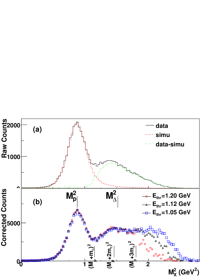
Two classes of inclusive hadronic electroproduction channels compete with the exclusive reaction: the channels, with a threshold at and the channel. The first class includes and non-resonant production in the final state, and diffractive production via the reaction. All these channels can be observed in a missing-mass squared distribution (Figure 6). The channel originates from the diffractive reaction, with a 8.5% branching-ratio decay channel Yao et al. (2006). In our acceptance, the missing-mass squared threshold for exclusive electroproduction is , thus slightly lower than the threshold of . However, based on measurements performed by Morand et al. (2005), the expected background of events for is less than 1% of the exclusive yield in all bins.
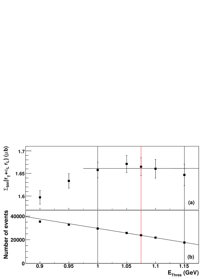
The systematic errors in the extraction method are due to the cut on the missing-mass squared and on the calorimeter threshold . The stability of the results is checked by varying each cut in turn. The variation in the estimator
| (33) |
is used to quantify the systematic errors.
-
i
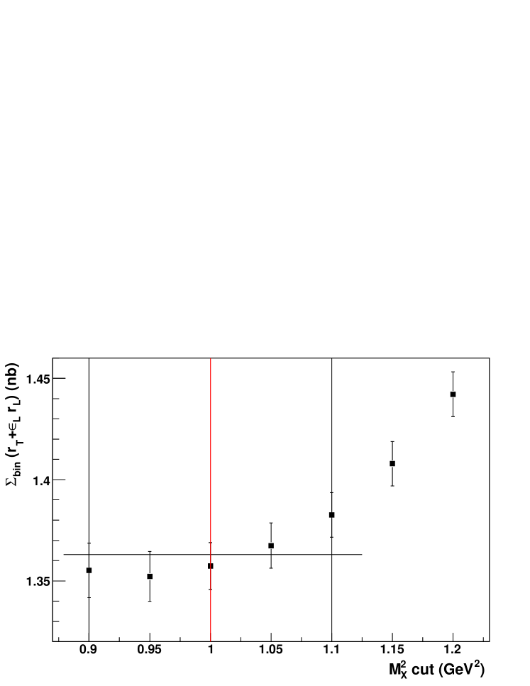
For the exclusivity () cut, we consider the stability interval from to GeV2 in the cut. At the high end we expect the cross section to have contributions from inelastic final states (Figure 6). At the low end, we are removing roughly half of the statistics, and we become progressively more sensitive to the experimental line shape. The stability of the exclusivity cut (e.g. for Kin3) is plotted in Figures 8. The cuts and variation are listed in Tables 4 and 5. In each case, this study is performed with fixed at 1.0 GeV.
-
ii
For the calorimeter threshold , the stability of is expected when the software threshold is fixed above the hardware threshold. Above the hardware threshold, the cut is directly correlated with the decay phase space, and the number of events decreases linearly with . This comes from the isotropic decay of the pion, leading to a flat energy distribution of each decay photon. Figure 9 shows for Kin2, the quantity along with the raw number of counts. The stability is indeed no longer observed when the statistics are not linear with the threshold, meaning the hardware threshold competes with the analysis threshold. The same behavior is shown for Kin3. For both kinematics, the systematic error coming from the calorimeter threshold is evaluated as .
The optimal cut is set in the middle of the stability interval (see Figures 8 and 9).The stability interval bounds and the optimal values for the cut and are listed in Table 4 for both kinematics.
| Variable | Minimum | Optimum | Maximum |
|---|---|---|---|
| Kin3/Kin3 | |||
| cut () | 0.90 | 1.00 | 1.10 |
| (GeV) | 1.20 | 1.275 | 1.35 |
| Kin2/Kin2 | |||
| cut () | 0.90 | 1.00 | 1.10 |
| (GeV) | 1.00 | 1.075 | 1.15 |
The reduced structure functions are extracted at the optimal value of the cuts. For the structure functions implied in dependences, systematic errors are taken as the rms difference between the computed at the optimum cuts and the computed at each of the four extremities of the stability domain.
All instrumental sources of systematic errors are shown along with the analysis systematic errors in Table 5.
| Kin3 | Kin2 | |
|---|---|---|
| Kin3 (%) | Kin2 (%) | |
| Exclusivity cut | 1.5 | 3.0 |
| Calorimeter threshold | 1.0 | |
| HRS acceptance | 2.2 | |
| Radiative corrections | 1.5 | |
| Target length | 0.5 | |
| Hadronic tensor integration | 0.3 | |
| Multitracks corrections | 0.1 | |
| 3 clusters corrections | 0.1 | |
| Luminosity | 0.1 | |
| Dead time | 0.1 | |
| Particle identification | 0.1 | |
| Total quadratic | 3.3 | 4.2 |
| Beam polarization | 2.0 | |
| Total quadratic | 3.9 | 4.6 |
VIII Results
The exclusive electroproduction cross section and, in particular, the dependences of its separated components were extracted for Kin2, Kin3, Kin2 and Kin3. Our statistics allowed us to achieve, for the -independent cross section, a statistical precision of 3% for Kin2 and Kin3, and of 5% for Kin2 and Kin3. This difference is due to the fact that we could use the full statistics for Kin2 and Kin3, whereas less than half of the statistics were available for Kin2 and Kin3.
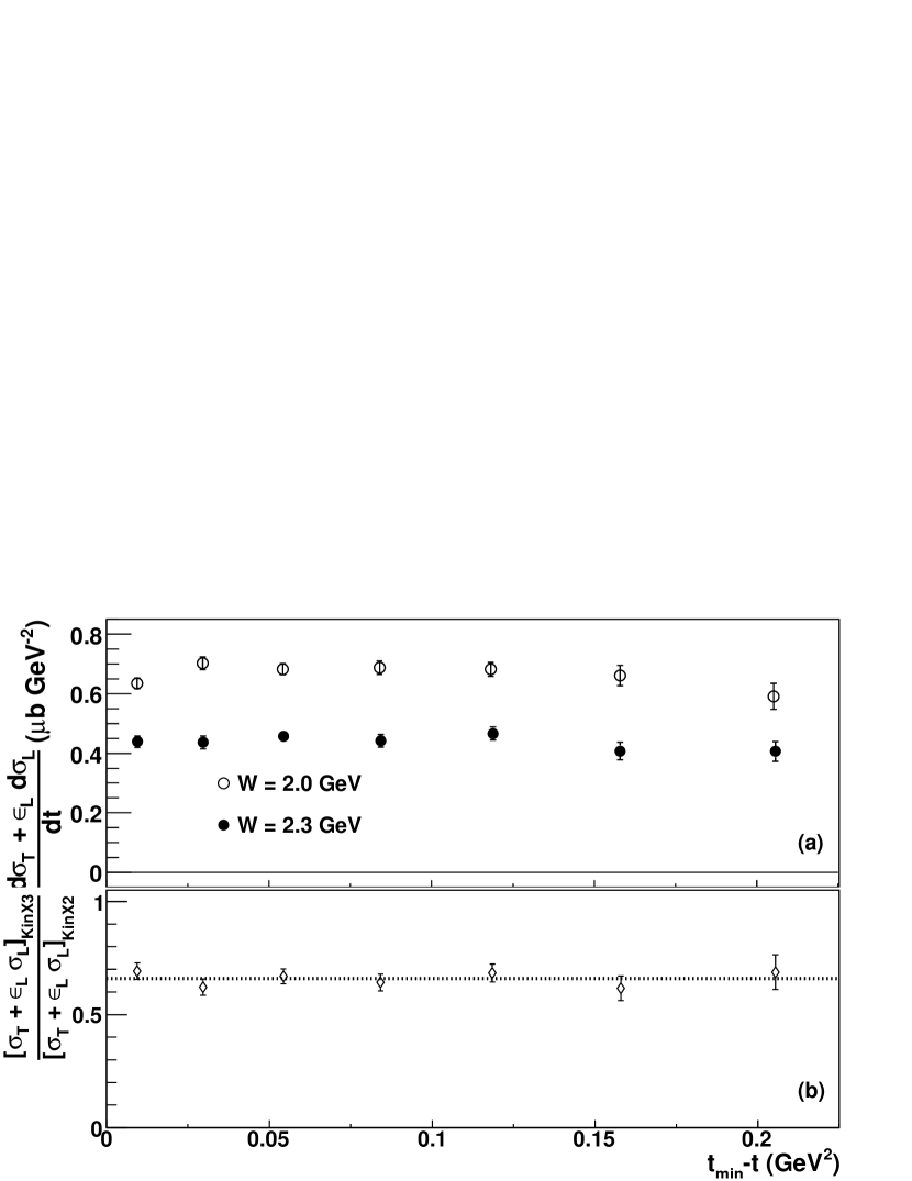
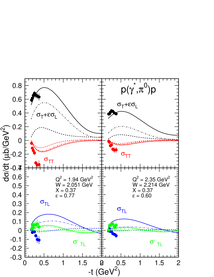
Figure 10 shows and Figure 11 shows , , and plotted as a function of , both for Kin2 and Kin3. Figure 12 shows and Figure 13 shows , , and , both for Kin2 and Kin3.

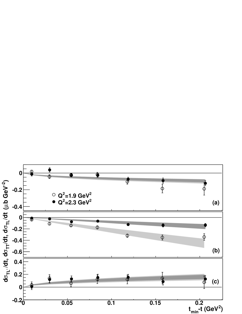
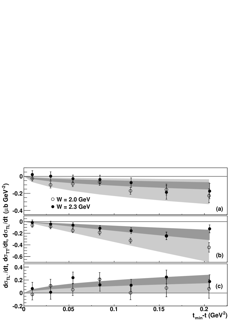
We performed fits proportional to for and , and proportional to for . These fits, including statistical and systematic errors, are shown as bands in Figures 11 and 13, and in Tables 11 and 12. Their reduced are below 1.05 for the -dependent data, and below 0.75 for the -dependent data. This confirms that the main dependence of , and is given by and , respectively.
The lower panel of Figure 10 (respectively, Figure 12) also shows the dependence (respectively, dependence) for the total cross section . To investigate a or a dependence, the ratio of for the two kinematics is plotted as a function of . This ratio is found to be independent of , thus the value of this ratio is fitted by a constant at the - and - values for the two kinematics.
The dependence of in Figures 10 and 12 yields the following conclusions:
-
i
The ratio is flat in with a reduced of 0.33. The ratio is found to be , indicating a dependence of the total cross section of about .
-
ii
The ratio is also flat in with a reduced of 0.56. This ratio is found to be , indicating a dependence of the total cross section of about .
The and dependences of the relevant quantities [, , and , with our conventions (i.e Drechsel-Tiator) and VGG conventions] have been summarized in Table 6.
| Quantity | dependence | dependence |
|---|---|---|
| (Drechsel-Tiator) | ||
| (VGG) |
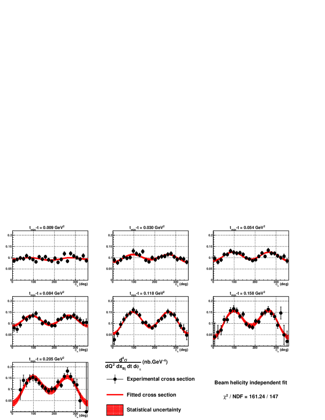
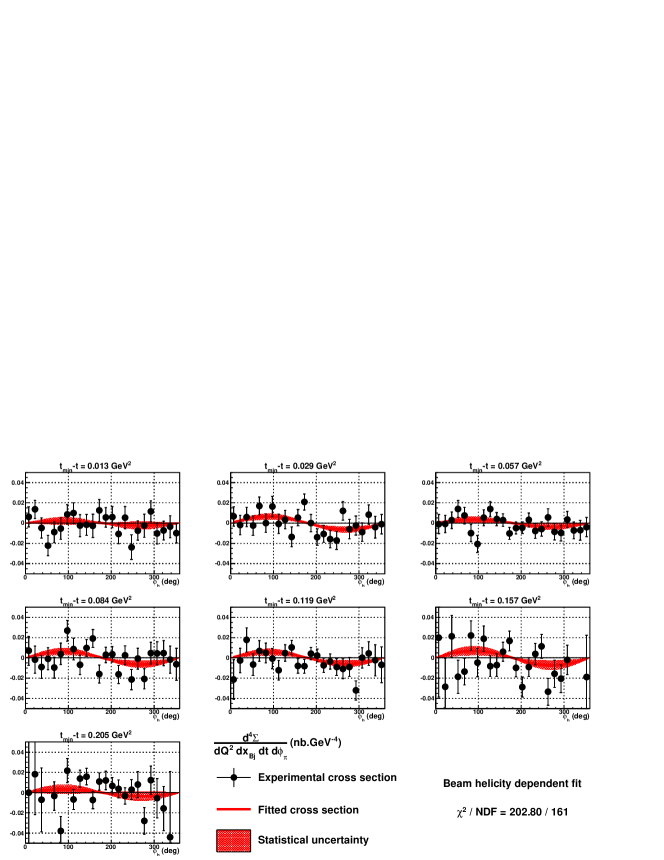
We extract the experimental cross sections
| (34) |
(respectively beam helicity independent and beam helicity dependent) for each bin in and . They are defined, for each vertex kinematic bin in terms of the yield in the corresponding bin as:
| (35) |
The experimental counts and simulation counts are defined previously in the text. The five-fold differential cross section are defined as
| (36) |
and
| (37) |
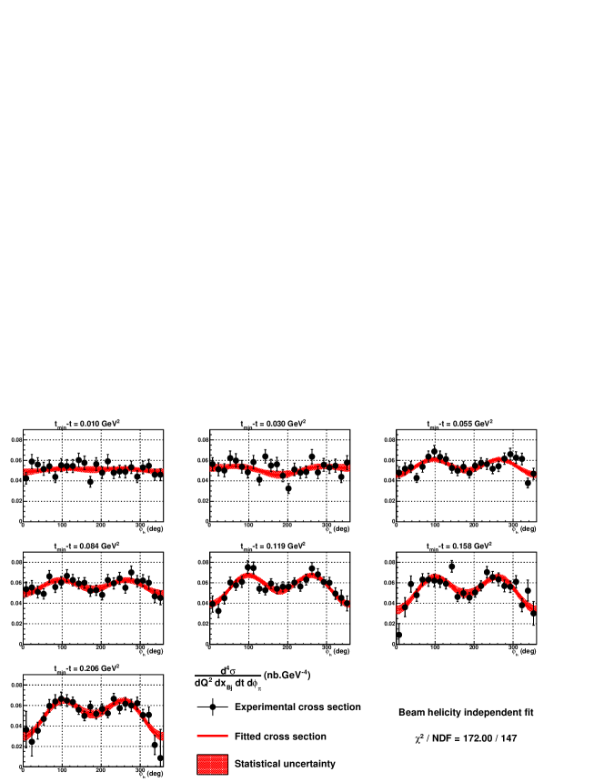
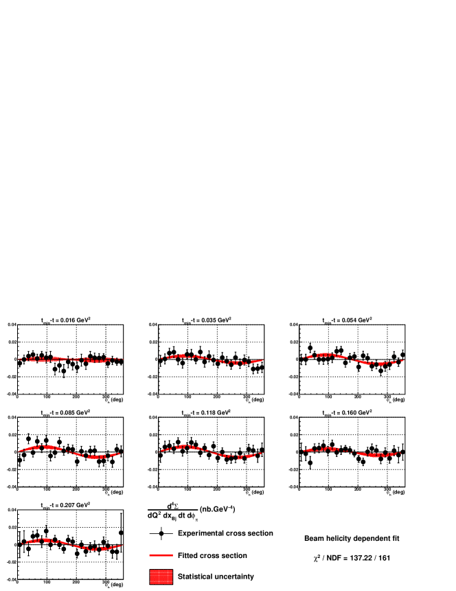
The experimental cross sections and are plotted in Figs. 16 and 17 and tabulated in Tables 13 and 14, respectively, for Kin2 (). Corresponding plots and tables are presented in Figs. 18 and 19 respectively, and Tables 15 and 16 for Kin3 ().
IX Discussion
In the domain in where we extracted cross sections, the values from Eqs. (15) and (16) are constant within statistics, as evidenced by the fits in Figures 11 and 13.
The data we extracted (see the previous section) yield two conclusions with regard to the available models:
- i
-
ii
the dependence of the cross section (Figure 10 and Table 6) demonstrates that we are far from the QCD leading twist prediction of , which behaves as . On the other hand, it is similar to the dependence of the transverse cross section for charged pion electroproduction published by Hall C Horn et al. (2008).
Moreover, the has no charge and no spin, so a direct coupling with a virtual photon is suppressed, which removes the pion-pole contribution to the longitudinal cross section. This suggests that the transverse cross section is likely to dominate, and transverse cross sections have already been described by quark fragmentation mechanisms usually used to describe semi-inclusive processes.
T. Horn et al. measured the exclusive electroproduction cross section at and , with and separation Horn et al. (2008). The -channel meson-exchange model by Laget reproduces the component. However, the component does not follow the TME model prediction. Kaskulov et al. performed pythia-jetset calculations using the Lund model applied to transverse cross sections at Hall C kinematics Kaskulov et al. (2008). In this model, the virtual photon strikes a quark, with a probability given by the structure functions. Due to this, the hadronic system fragments into two jets. The jet engendered by the single quark gives a pion, and the one engendered by the remainder of the nucleon gives the final neutron. These calculations applied to Hall C transverse cross sections are in excellent agreement with the data. This gives evidence that the transverse cross section at above the resonance region is described by a partonic process. This suggests that the present data could similarly be described by incoherent scattering on the partonic structure of the nucleon target.
For these reasons, we consider our data within the context of semi-inclusive deep inelastic scattering (SIDIS). We can try to fit our data with a SIDIS formalism written by Anselmino et al. Anselmino et al. (2005). Equation (38) of Anselmino et al. (2005) gives the cross section for semi-inclusive production of a pion (valid for any hadron):
| (38) | ||||
where , and is the fraction of the reaction energy carried by the measured hadron, and the quantities between angle brackets are the standard deviations of transverse momentum distributions, which are approximated as Gaussian. stands for the parton transverse momentum in the proton, and is the measured transverse momentum of the observed hadron, where stands for the transverse momentum of the hadron with respect to the direction of the struck quark. The idea is to adjust the ratio of over constant term in brackets of Eq. (38) by adjusting only the parameter :
| (39) |
Two conclusions arise from the fits shown in Figure 15: (1) the minus sign affecting the term in the SIDIS model is in agreement with the and (2) must be equal to to reproduce the data.
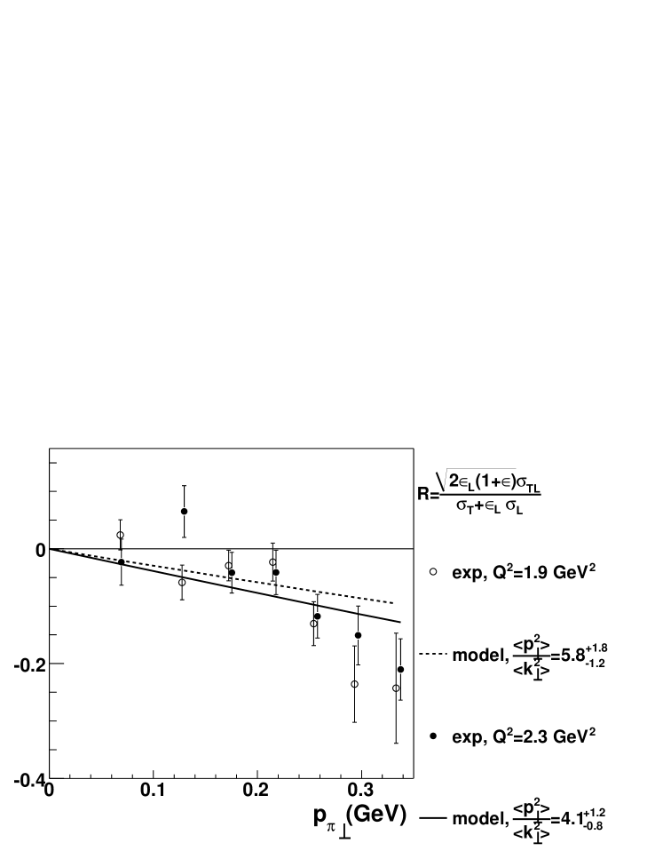
The authors of Anselmino et al. (2005) adjusted their model to semi-inclusive data. They give and , giving a ratio . However, they extracted these values in the inclusive region, implying a high multiplicity of particles, whereas in our data, the multiplicity of particles is unity. Typically, Anselmino et al. fit their model with data covering the range , with most of the statistics within , whereas our data are within . Furthermore, Kaskulov et al. Kaskulov et al. (2008) used a value of 1.4 for the rms transverse momentum of partons in their fit of the Hall C data. The exclusive limit of SIDIS could be defined by a SIDIS-inspired model applicable to data at or, more practically, when the measured hadron carries such a large fraction of the total energy of the reaction that it does not allow the production of another particle.
The HERMES and COMPASS collaborations have published moments of and SIDIS, including up to 0.7 Barone et al. (2010).
However, it is not possible to make a direct comparison to our data as the and moments on the proton have different signs and magnitudes for Boer-Mulders effect.
On the other hand, the higher twist Cahn effect, which also contributes to , does not give by itself a satisfying description of .
X Conclusions
We extracted the separated differential cross section at Jefferson Lab, Hall A, at four kinematic settings: Kin2 and Kin3 with a 3% statistical precision, and Kin2 and Kin3 with a 5% statistical precision. We studied the dependence of the hadronic tensor with the two first settings, and the dependence with the latter two.
The shape and order of magnitude of the cross section componants indicate that the -channel meson-exchange model is able to reproduce the total cross section, but it would still need improvement for the description of the other components.
Table 6 summarizes the contradiction between our data and the leading twist QCD prediction for high . Instead of an dependence we find, under the assumption that is negligible (which is very unlikely), a dependence for . On the other hand, the cross section extracted may show an analogy with the formalism of SIDIS at the exclusive limit. Our data, and the Hall C data are important bases for studying the applicability of the SIDIS concepts to exclusive data. To improve the understanding of our data, we have run another experiment in Fall 2010, at two beam energies, allowing us to disentangle from .
We acknowledge the essential work of the JLab accelerator division and the Hall A technical staff. This work was supported by DOE Contract No. DOE-AC05-06OR23177 under which the Jefferson Science Associates, LLC, operates the Thomas Jefferson National Accelerator Facility. We acknowledge additional grants from DOE, NSF, and the French CNRS, ANR, and Commissariat à l’ Energie Atomique.
References
- Goldstein and Owens (1973) G. R. Goldstein and J. F. Owens, Phys. Rev. D7, 865 (1973).
- Guidal et al. (1997a) M. Guidal, J. M. Laget, and M. Vanderhaeghen, Nucl. Phys. A627, 645 (1997a).
- Guidal et al. (1997b) M. Guidal, J. M. Laget, and M. Vanderhaeghen, Phys. Lett. B400, 6 (1997b).
- De Masi et al. (2008) R. De Masi et al. (CLAS), Phys. Rev. C77, 042201 (2008).
- Laget (2007) J. M. Laget, Phys. Rev. C76, 052201 (2007).
- Laget (2011) J. M. Laget, Phys. Lett. B695, 199 (2011).
- Ahmad et al. (2009) S. Ahmad, G. R. Goldstein, and S. Liuti, Phys. Rev. D79, 054014 (2009).
- Horn et al. (2008) T. Horn et al., Phys. Rev. C78, 058201 (2008).
- Collins et al. (1997) J. C. Collins, L. Frankfurt, and M. Strikman, Phys. Rev. D56, 2982 (1997).
- Goeke et al. (2001) K. Goeke, M. V. Polyakov, and M. Vanderhaeghen, Prog. Part. Nucl. Phys. 47, 401 (2001).
- Vanderhaeghen et al. (1999) M. Vanderhaeghen, P. A. M. Guichon, and M. Guidal, Phys. Rev. D60, 094017 (1999).
- Mueller et al. (1994) D. Mueller, D. Robaschik, B. Geyer, F. M. Dittes, and J. Horejsi, Fortschr. Phys. 42, 101 (1994).
- Ji (1997) X.-D. Ji, Phys. Rev. Lett. 78, 610 (1997).
- Radyushkin (1997) A. V. Radyushkin, Phys. Rev. D56, 5524 (1997).
- Kaskulov et al. (2008) M. M. Kaskulov, K. Gallmeister, and U. Mosel, Phys. Rev. D78, 114022 (2008).
- Drechsel and Tiator (1992) D. Drechsel and L. Tiator, J. Phys. G18, 449 (1992).
- Bertin et al. (2000) P. Y. Bertin, C. E. Hyde, R. Ransome, and F. Sabatié, Jefferson Lab Proposal, E00-110, Jefferson Lab (2000).
- Muñoz Camacho (2005) C. Muñoz Camacho, Ph.D. thesis, Université Paris VI, France (2005).
- Munoz Camacho et al. (2006) C. Munoz Camacho et al. (Jefferson Lab Hall A), Phys. Rev. Lett. 97, 262002 (2006).
- Mazouz and Voutier (2005) M. Mazouz and E. Voutier, Hall A Technical Note Jlab-TN-05-033, Jefferson Lab (2005), URL http://hallaweb.jlab.org/publications/Technotes/technote.html%.
- Kelly (2004) J. J. Kelly, Phys. Rev. C70, 068202 (2004).
- Chew et al. (1957) G. F. Chew, M. L. Goldberger, F. E. Low, and Y. Nambu, Phys. Rev. 106, 1345 (1957).
- Rvachev (2001) M. Rvachev, Hall A Technical Note Jlab-TN-01-055, Jefferson Lab (2001), URL http://hallaweb.jlab.org/publications/Technotes/technote.html%.
- Mo and Tsai (1969) L. W. Mo and Y.-S. Tsai, Rev. Mod. Phys. 41, 205 (1969).
- Tsai (1974) Y.-S. Tsai, Rev. Mod. Phys. 46, 815 (1974).
- Vanderhaeghen et al. (2000) M. Vanderhaeghen, J. M. J. M. Friedrich, D. Lhuillier, D. Marchand, L. VanHoorebeke, and J. VandeWiele, Phys. Rev. C62, 025501 (2000).
- Yao et al. (2006) W. M. Yao et al. (Particle Data Group), J. Phys. G33, 1 (2006).
- Morand et al. (2005) L. Morand et al. (CLAS), Eur. Phys. J. A24, 445 (2005).
- Anselmino et al. (2005) M. Anselmino, M. Boglione, U. D’Alesio, A. Kotzinian, F. Murgia, and A. Prokudin, Phys. Rev. D71, 074006 (2005).
- Barone et al. (2010) V. Barone, S. Melis, and A. Prokudin, Phys. Rev. D82, 114025 (2010).
| dependence | dependence | |||
| Kin3 | Kin2 | Kin3 | Kin2 | |
| 15516 | 23429 | 5952 | 9860 | |
| nb-1 | nb-1 | |||
| () | ||||
| (GeV) | ||||
| () | ||||
| (GeV) | ||||
| (GeV) | ||||
| (GeV) | ||||
| (GeV) | ||||
| (GeV) | ||||
| dependence | dependence | ||||
|---|---|---|---|---|---|
| () | () | ||||
| Kin3 | Kin3 | ||||
| 0.0095 | 0.077 | 0.007 | 0.0095 | 0.076 | 0.007 |
| 0.0298 | 0.144 | 0.021 | 0.0297 | 0.143 | 0.020 |
| 0.0546 | 0.194 | 0.038 | 0.0545 | 0.193 | 0.037 |
| 0.0844 | 0.241 | 0.058 | 0.0843 | 0.240 | 0.058 |
| 0.1188 | 0.285 | 0.081 | 0.1188 | 0.284 | 0.081 |
| 0.1583 | 0.328 | 0.108 | 0.1579 | 0.326 | 0.106 |
| 0.2063 | 0.372 | 0.139 | 0.2057 | 0.370 | 0.137 |
| Kin2 | Kin2 | ||||
| 0.0094 | 0.085 | 0.008 | 0.0094 | 0.085 | 0.008 |
| 0.0296 | 0.159 | 0.026 | 0.0296 | 0.160 | 0.026 |
| 0.0541 | 0.215 | 0.046 | 0.0542 | 0.216 | 0.047 |
| 0.0839 | 0.267 | 0.071 | 0.0840 | 0.268 | 0.072 |
| 0.1179 | 0.315 | 0.099 | 0.1181 | 0.316 | 0.100 |
| 0.1576 | 0.362 | 0.131 | 0.1579 | 0.364 | 0.133 |
| 0.2050 | 0.410 | 0.168 | 0.2051 | 0.412 | 0.170 |
| dependence | ||
|---|---|---|
| Kin3 | Kin2 | |
| , | , | |
| 0.010 | 377 10 12 | 571 10 24 |
| 0.030 | 381 12 12 | 600 12 25 |
| 0.054 | 403 10 13 | 641 12 27 |
| 0.084 | 425 11 14 | 673 15 28 |
| 0.118 | 418 11 14 | 645 16 27 |
| 0.158 | 395 13 13 | 636 25 27 |
| 0.206 | 384 13 13 | 628 36 26 |
| 0.010 | -13 23 10 | 17 19 13 |
| 0.030 | 38 26 24 | -43 22 12 |
| 0.054 | -25 22 11 | -23 21 12 |
| 0.084 | -26 25 13 | -19 27 14 |
| 0.118 | -75 24 9 | -103 30 21 |
| 0.158 | -91 30 8 | -185 52 43 |
| 0.206 | -123 31 10 | -189 74 34 |
| 0.010 | -12 23 14 | -39 19 7 |
| 0.030 | -25 27 15 | -110 24 13 |
| 0.054 | -74 22 4 | -141 22 17 |
| 0.084 | -64 25 14 | -174 28 17 |
| 0.118 | -124 24 16 | -319 29 23 |
| 0.158 | -137 29 15 | -352 45 53 |
| 0.206 | -134 30 15 | -343 57 68 |
| 0.010 | 9 49 20 | 31 51 15 |
| 0.030 | 119 55 21 | 136 61 24 |
| 0.054 | 129 46 12 | 61 56 41 |
| 0.084 | 151 51 30 | 123 68 20 |
| 0.118 | 153 47 17 | 120 69 24 |
| 0.158 | 87 54 23 | 142 91 36 |
| 0.206 | 127 51 15 | 76 99 80 |
| dependence | ||
|---|---|---|
| Kin3 | Kin2 | |
| , | , | |
| 0.010 | 439 19 14 | 635 17 26 |
| 0.030 | 437 22 14 | 703 21 29 |
| 0.054 | 457 18 15 | 683 19 28 |
| 0.084 | 442 21 14 | 688 23 29 |
| 0.118 | 466 22 15 | 682 23 28 |
| 0.158 | 407 29 13 | 662 34 28 |
| 0.205 | 406 34 13 | 591 44 25 |
| 0.010 | 20 46 38 | -26 30 22 |
| 0.030 | 2 50 17 | -100 37 61 |
| 0.054 | -28 43 15 | -88 32 54 |
| 0.084 | -37 50 19 | -68 38 487 |
| 0.118 | -74 55 27 | -170 40 562 |
| 0.158 | -188 80 27 | -155 63 657 |
| 0.205 | -174 90 32 | -228 82 738 |
| 0.010 | -16 44 16 | -63 33 18 |
| 0.030 | -44 50 32 | -83 41 22 |
| 0.054 | -63 42 15 | -153 36 24 |
| 0.084 | -114 47 8 | -186 43 78 |
| 0.118 | -156 50 18 | -327 44 109 |
| 0.158 | -244 66 35 | -247 65 141 |
| 0.205 | -124 69 42 | -444 82 183 |
| 0.010 | 68 97 35 | -23 84 138 |
| 0.030 | 12 109 39 | 112 100 104 |
| 0.054 | 236 88 19 | 50 90 63 |
| 0.084 | 126 99 26 | 211 104 95 |
| 0.118 | 119 93 22 | 3 106 111 |
| 0.158 | 246 106 89 | 78 136 126 |
| 0.205 | 177 104 30 | 62 146 146 |
| dependence |
|---|
| Kin3 = 0.368, = 2.350 () |
| nb |
| nb |
| nb |
| Kin2 = 0.368, = 1.941 () |
| nb |
| nb |
| nb |
| dependence |
|---|
| Kin3 = 0.335, = 2.155 () |
| nb |
| nb |
| nb |
| Kin2 = 0.394, = 2.073 () |
| nb |
| nb |
| nb |
| (pb ) | |||||||
|---|---|---|---|---|---|---|---|
| 0.010 | 0.030 | 0.054 | 0.084 | 0.118 | 0.158 | 0.205 | |
| (deg) | |||||||
| 7.5 | 86.15 7.85 | 89.61 8.85 | 96.38 10.50 | 80.59 14.74 | 28.16 21.64 | 41.38 61.01 | -715.48 314.53 |
| 22.5 | 92.60 7.63 | 77.79 8.45 | 80.61 8.76 | 74.07 13.41 | 54.94 13.63 | 62.17 30.56 | -99.56 72.94 |
| 37.5 | 98.69 8.10 | 90.27 8.51 | 90.50 8.34 | 93.88 10.85 | 95.93 13.41 | 70.65 20.83 | 98.36 43.24 |
| 52.5 | 95.41 7.93 | 103.59 8.51 | 114.50 8.21 | 126.75 10.17 | 117.93 11.39 | 117.19 16.01 | 139.95 23.66 |
| 67.5 | 108.24 8.28 | 97.84 8.01 | 114.29 8.02 | 118.34 9.42 | 136.07 10.91 | 116.74 12.84 | 127.45 17.11 |
| 82.5 | 98.59 7.91 | 101.02 8.34 | 129.87 8.29 | 129.04 9.66 | 146.51 10.23 | 157.22 13.93 | 147.81 16.72 |
| 97.5 | 91.64 7.19 | 130.36 9.55 | 123.92 8.25 | 135.90 9.49 | 160.29 10.57 | 165.46 13.51 | 152.67 14.22 |
| 112.5 | 81.80 7.21 | 118.51 8.91 | 120.10 7.99 | 145.20 9.45 | 151.23 10.09 | 157.42 12.08 | 143.44 12.22 |
| 127.5 | 104.15 7.94 | 111.95 8.49 | 121.61 7.78 | 122.87 8.50 | 137.51 8.58 | 131.98 9.92 | 128.34 10.54 |
| 142.5 | 93.66 7.44 | 127.54 9.00 | 114.98 7.25 | 99.98 7.21 | 104.60 7.31 | 141.27 10.78 | 113.38 10.26 |
| 157.5 | 103.97 8.03 | 88.87 7.30 | 99.26 6.58 | 109.08 7.64 | 104.67 7.35 | 98.20 9.08 | 103.00 11.04 |
| 172.5 | 90.92 7.30 | 81.68 7.15 | 94.38 6.53 | 100.86 7.47 | 90.42 6.79 | 87.99 8.87 | 92.65 11.24 |
| 187.5 | 84.70 6.80 | 100.32 7.97 | 86.94 6.30 | 89.97 6.74 | 80.05 6.36 | 82.72 8.52 | 101.53 11.29 |
| 202.5 | 97.63 7.66 | 91.05 7.56 | 90.84 6.27 | 90.54 6.71 | 89.67 6.46 | 110.74 9.44 | 102.94 10.49 |
| 217.5 | 79.67 7.02 | 99.86 7.57 | 106.18 7.21 | 116.88 7.84 | 111.76 7.34 | 107.67 8.79 | 133.04 11.09 |
| 232.5 | 92.30 7.66 | 105.19 8.15 | 120.98 7.46 | 121.08 8.19 | 121.82 7.93 | 142.67 10.09 | 117.56 9.62 |
| 247.5 | 117.79 8.60 | 107.01 8.34 | 106.08 7.19 | 135.68 8.99 | 132.76 8.80 | 149.91 11.29 | 157.60 12.06 |
| 262.5 | 84.96 7.24 | 114.61 8.69 | 133.27 8.49 | 126.02 9.27 | 153.31 10.42 | 162.73 12.93 | 181.18 15.27 |
| 277.5 | 119.19 8.59 | 118.22 8.89 | 119.60 7.89 | 128.61 9.19 | 141.31 9.89 | 144.08 12.87 | 157.05 15.51 |
| 292.5 | 107.80 8.17 | 104.11 8.50 | 119.42 7.86 | 137.31 9.89 | 138.58 10.12 | 130.68 13.05 | 131.01 17.41 |
| 307.5 | 100.35 8.19 | 92.51 8.16 | 108.65 7.92 | 126.16 10.50 | 116.46 10.96 | 92.60 14.06 | 119.71 25.71 |
| 322.5 | 93.52 7.74 | 97.68 8.32 | 100.23 8.36 | 115.51 11.82 | 90.45 12.86 | 146.81 27.39 | 49.27 34.24 |
| 337.5 | 108.63 8.83 | 94.20 9.35 | 106.68 9.80 | 103.77 13.15 | 77.24 17.57 | 49.70 42.59 | -31.50 92.90 |
| 352.5 | 87.30 7.66 | 80.61 8.34 | 86.20 9.59 | 105.08 15.92 | 48.56 21.05 | 20.91 45.96 | 0.00 297.59 |
| (pb ) | |||||||
|---|---|---|---|---|---|---|---|
| 0.010 | 0.030 | 0.054 | 0.084 | 0.118 | 0.158 | 0.205 | |
| (deg) | |||||||
| 7.5 | 6.22 9.89 | 6.66 9.58 | -0.95 9.54 | 6.96 14.43 | -21.24 19.59 | 19.83 58.48 | 0.00 83.84 |
| 22.5 | 13.62 8.98 | -1.88 9.61 | -0.83 8.52 | -1.80 13.36 | -2.54 11.96 | -28.44 27.95 | 18.26 40.13 |
| 37.5 | -4.77 9.85 | 6.06 9.55 | 2.85 8.15 | -8.86 11.27 | 17.72 11.97 | 21.20 20.84 | -7.14 31.40 |
| 52.5 | -22.18 10.06 | -2.40 9.55 | 13.96 8.39 | -0.88 10.88 | -6.61 10.58 | -18.57 16.35 | 50.01 17.36 |
| 67.5 | -8.76 10.42 | 16.95 8.89 | 7.42 8.21 | -9.60 10.25 | 6.93 10.18 | -13.60 13.17 | -3.34 14.12 |
| 82.5 | -5.25 10.67 | 0.00 9.03 | -9.81 8.45 | 3.90 10.57 | 4.84 9.71 | 22.12 14.41 | -37.69 13.98 |
| 97.5 | 8.59 9.74 | 16.34 10.20 | -20.57 8.36 | 26.79 10.43 | -0.68 10.02 | -4.69 13.89 | 21.67 11.91 |
| 112.5 | 9.82 10.23 | -0.72 9.51 | 5.29 7.88 | 8.63 10.73 | -12.19 9.54 | 18.78 12.60 | -6.81 9.93 |
| 127.5 | -2.50 10.92 | 3.57 9.16 | 13.88 7.41 | -6.90 9.68 | 4.76 8.16 | -8.10 10.35 | 13.84 8.41 |
| 142.5 | -1.66 10.30 | -13.54 9.86 | 3.96 6.62 | 9.76 8.27 | 10.18 7.04 | -7.14 11.30 | 15.87 8.27 |
| 157.5 | -2.69 11.50 | 5.39 8.09 | 2.95 6.18 | 19.20 8.79 | -7.88 7.19 | 6.10 9.42 | -7.29 8.50 |
| 172.5 | 12.55 10.79 | 20.88 7.92 | -10.16 5.94 | -16.02 8.85 | -8.24 6.77 | 16.64 9.77 | 10.93 8.68 |
| 187.5 | 5.75 9.62 | -0.00 8.67 | -4.74 5.87 | 2.99 7.56 | 4.24 5.99 | -9.89 8.62 | 12.12 9.10 |
| 202.5 | 5.92 10.56 | -13.81 8.20 | -4.44 5.65 | 3.54 7.61 | 2.37 6.29 | -28.85 9.91 | 6.79 8.04 |
| 217.5 | -10.71 9.58 | -10.63 8.47 | 3.24 6.85 | -16.26 8.97 | -7.26 7.02 | -9.08 9.20 | 3.71 8.84 |
| 232.5 | 5.40 10.90 | -15.68 8.78 | -7.76 7.15 | 2.58 9.26 | -3.52 7.54 | 3.77 10.55 | -3.27 8.13 |
| 247.5 | -23.68 12.10 | -17.05 8.95 | -5.79 7.04 | -21.38 10.05 | -8.87 8.30 | 11.32 11.74 | 3.03 9.85 |
| 262.5 | -7.44 9.51 | 12.09 9.22 | 5.55 8.62 | -0.74 10.28 | -10.78 9.85 | -33.46 13.21 | 7.86 12.97 |
| 277.5 | -2.49 11.48 | -5.96 9.63 | -8.60 8.08 | -20.65 10.12 | -9.05 9.36 | -15.67 13.30 | -27.89 13.06 |
| 292.5 | 11.69 10.39 | -2.32 9.35 | -9.74 7.87 | 4.62 10.75 | -32.10 9.53 | -20.57 13.61 | 12.17 13.95 |
| 307.5 | -10.15 10.42 | -8.83 9.20 | 3.56 8.00 | 4.55 11.28 | 0.00 10.17 | -1.99 14.53 | -5.51 19.51 |
| 322.5 | -7.31 9.35 | 8.48 9.46 | -7.16 8.36 | 4.66 12.28 | 4.34 11.72 | 57.34 27.10 | -15.68 21.79 |
| 337.5 | -3.58 10.91 | -3.86 10.72 | -7.04 9.78 | -1.68 13.42 | -2.41 15.33 | -93.25 39.96 | -44.06 64.96 |
| 352.5 | -9.92 9.65 | -0.98 9.64 | -3.94 9.53 | -6.38 15.77 | -6.82 17.74 | -18.77 41.25 | 95.20 229.23 |
| (pb ) | |||||||
|---|---|---|---|---|---|---|---|
| 0.010 | 0.030 | 0.054 | 0.084 | 0.118 | 0.158 | 0.205 | |
| (deg) | |||||||
| 7.5 | 42.30 5.51 | 56.32 6.40 | 47.89 5.81 | 53.76 7.07 | 39.42 7.95 | 9.15 11.23 | 36.28 17.85 |
| 22.5 | 58.86 6.82 | 51.25 6.35 | 51.82 5.84 | 55.51 6.82 | 32.64 6.49 | 36.22 9.29 | 24.49 13.91 |
| 37.5 | 55.99 6.54 | 50.20 6.37 | 53.57 5.37 | 51.23 5.81 | 45.17 5.76 | 58.82 7.94 | 35.29 8.23 |
| 52.5 | 51.60 6.34 | 62.06 7.00 | 42.86 4.45 | 49.20 5.10 | 60.24 5.42 | 47.96 5.86 | 46.77 5.90 |
| 67.5 | 54.11 6.32 | 59.86 6.54 | 53.64 5.20 | 66.28 5.79 | 57.54 5.06 | 63.18 5.80 | 59.44 6.30 |
| 82.5 | 43.79 5.47 | 53.80 6.28 | 63.64 5.45 | 55.86 5.19 | 60.93 5.41 | 63.16 6.41 | 63.73 6.79 |
| 97.5 | 55.28 6.36 | 48.47 5.78 | 68.73 5.80 | 60.38 5.66 | 75.30 6.15 | 62.20 6.06 | 66.39 6.56 |
| 112.5 | 54.48 6.32 | 58.22 6.53 | 63.38 5.67 | 66.92 5.94 | 74.56 5.71 | 61.21 5.72 | 64.68 5.76 |
| 127.5 | 54.37 6.22 | 41.12 5.22 | 61.10 5.44 | 62.61 5.62 | 54.38 4.50 | 59.08 5.12 | 63.22 4.92 |
| 142.5 | 60.22 6.67 | 63.82 6.48 | 52.46 4.90 | 59.45 5.48 | 52.72 4.53 | 76.04 5.64 | 55.82 4.53 |
| 157.5 | 57.59 6.54 | 54.90 6.04 | 49.94 4.87 | 60.05 5.20 | 59.28 4.72 | 46.22 4.44 | 49.73 4.67 |
| 172.5 | 38.95 5.26 | 56.20 6.59 | 53.68 5.04 | 52.13 5.21 | 54.33 4.78 | 49.83 5.03 | 58.60 5.40 |
| 187.5 | 56.32 6.32 | 44.95 5.85 | 47.40 4.57 | 52.82 5.12 | 56.14 4.94 | 45.60 4.75 | 51.81 5.26 |
| 202.5 | 47.94 5.81 | 32.41 4.80 | 54.65 5.22 | 48.15 4.79 | 56.11 4.60 | 50.68 4.69 | 56.62 4.92 |
| 217.5 | 59.05 6.66 | 51.08 6.13 | 57.24 5.16 | 62.73 5.63 | 60.22 4.73 | 57.02 4.96 | 52.17 4.35 |
| 232.5 | 48.04 5.95 | 47.92 5.60 | 56.26 5.21 | 59.48 5.41 | 56.52 4.70 | 70.51 5.57 | 66.53 5.13 |
| 247.5 | 49.20 5.91 | 48.71 5.69 | 51.84 4.91 | 64.47 5.74 | 63.20 5.23 | 65.54 5.57 | 57.32 5.33 |
| 262.5 | 48.85 6.10 | 63.63 6.95 | 54.14 5.06 | 55.34 5.34 | 74.01 5.77 | 63.37 6.23 | 61.63 6.12 |
| 277.5 | 53.33 6.02 | 48.07 6.01 | 61.57 5.55 | 70.15 6.30 | 68.22 5.50 | 57.00 5.75 | 59.99 5.99 |
| 292.5 | 44.06 5.84 | 55.57 6.31 | 66.06 5.66 | 61.62 5.70 | 60.79 5.11 | 56.24 5.59 | 62.01 6.00 |
| 307.5 | 53.08 6.20 | 53.08 5.99 | 62.68 5.67 | 62.24 5.71 | 60.01 5.38 | 61.06 6.04 | 50.40 5.76 |
| 322.5 | 54.68 6.38 | 54.79 6.35 | 61.38 5.68 | 60.12 6.31 | 49.55 5.68 | 38.16 6.38 | 50.64 7.87 |
| 337.5 | 46.01 5.53 | 43.90 5.72 | 37.90 4.73 | 46.75 6.09 | 45.29 7.48 | 52.43 10.29 | 21.25 9.45 |
| 352.5 | 45.97 5.84 | 57.70 6.92 | 46.95 5.44 | 45.29 6.71 | 39.98 7.38 | 30.17 11.50 | 8.57 27.98 |
| (pb ) | |||||||
|---|---|---|---|---|---|---|---|
| 0.010 | 0.030 | 0.054 | 0.084 | 0.118 | 0.158 | 0.205 | |
| (deg) | |||||||
| 7.5 | -4.24 4.00 | -1.50 6.31 | 0.00 6.02 | -9.23 6.92 | -3.75 8.07 | -0.00 10.41 | -0.00 15.07 |
| 22.5 | 0.00 5.06 | 0.72 5.78 | 0.00 5.94 | -3.26 6.60 | 5.80 6.73 | -1.73 8.00 | 3.65 12.44 |
| 37.5 | 3.81 5.34 | 7.21 5.77 | 13.33 5.45 | 15.34 5.73 | 7.19 5.96 | -12.24 7.12 | -4.80 7.83 |
| 52.5 | 5.55 4.57 | 8.48 6.37 | 4.87 4.49 | -0.53 5.07 | 3.98 5.69 | 4.27 5.37 | 9.53 5.84 |
| 67.5 | 1.18 4.91 | -0.00 5.88 | 0.00 5.22 | 12.24 5.76 | 11.45 5.25 | 4.64 5.43 | 10.59 6.34 |
| 82.5 | 4.73 4.43 | -4.11 5.84 | 0.00 5.45 | 4.58 5.20 | 1.01 5.55 | 7.43 5.97 | 3.59 6.88 |
| 97.5 | 2.12 6.18 | 5.75 5.33 | 0.51 5.76 | 13.43 5.64 | 4.58 6.27 | 1.17 5.59 | 15.58 6.67 |
| 112.5 | 2.92 6.25 | 5.52 6.11 | 2.06 5.63 | -4.29 5.90 | 11.13 5.79 | 8.64 5.22 | 0.00 5.91 |
| 127.5 | -11.02 6.67 | 0.00 4.87 | 9.37 5.32 | -0.51 5.56 | 8.43 4.55 | -0.41 4.53 | 5.69 5.06 |
| 142.5 | -6.81 7.63 | 8.58 6.36 | 10.28 4.80 | 11.39 5.38 | -0.77 4.53 | 2.28 4.94 | -0.00 4.64 |
| 157.5 | -13.29 7.55 | -2.77 5.93 | -3.90 4.80 | 1.43 5.07 | 4.74 4.74 | 3.78 3.81 | -4.98 4.71 |
| 172.5 | -2.83 6.75 | 3.61 6.35 | 1.92 4.91 | 3.74 5.12 | -3.29 4.66 | 2.07 4.13 | 5.23 5.44 |
| 187.5 | -5.38 6.63 | -0.71 5.67 | 3.54 4.36 | 3.02 5.03 | 6.66 5.00 | -1.61 3.94 | 3.32 5.23 |
| 202.5 | -8.93 5.95 | -4.83 4.71 | -8.45 5.13 | -10.90 4.67 | -6.67 4.63 | -7.90 3.93 | -10.26 5.01 |
| 217.5 | -0.78 6.85 | 2.08 5.90 | 4.35 5.06 | 1.00 5.48 | 0.00 4.74 | -11.32 4.30 | 0.00 4.44 |
| 232.5 | -4.80 6.44 | -1.93 5.34 | 1.43 5.11 | -4.06 5.35 | -8.49 4.74 | 0.42 5.07 | -7.76 5.25 |
| 247.5 | 3.58 5.60 | -5.90 5.28 | -7.70 4.87 | 1.07 5.72 | -7.42 5.28 | 4.07 5.15 | -3.10 5.47 |
| 262.5 | 1.96 5.30 | 2.11 6.47 | -5.69 5.00 | 1.58 5.33 | -6.25 5.85 | 1.74 5.81 | -1.86 6.28 |
| 277.5 | 1.78 4.95 | -4.86 5.47 | -12.96 5.57 | -10.76 6.30 | -0.93 5.64 | -7.87 5.45 | -5.52 6.07 |
| 292.5 | 2.65 4.07 | -0.68 5.79 | -7.83 5.70 | -10.24 5.69 | -7.27 5.27 | -0.53 5.25 | 2.88 6.09 |
| 307.5 | -4.44 4.73 | -2.59 5.49 | -5.73 5.75 | -4.25 5.65 | 3.41 5.59 | -7.13 5.53 | -1.28 5.70 |
| 322.5 | -1.08 4.73 | -10.89 5.68 | 3.20 5.77 | -11.24 6.17 | 1.89 5.85 | 1.63 5.73 | -8.01 7.47 |
| 337.5 | -2.52 4.06 | -10.54 5.06 | -3.00 4.80 | 3.05 5.86 | -4.18 7.75 | -3.38 8.94 | -8.23 8.54 |
| 352.5 | -2.73 3.47 | -9.09 5.96 | 5.49 5.37 | 0.84 6.38 | 2.62 7.74 | 0.00 9.42 | 13.67 22.30 |