11institutetext: Niels Bohr Institute & Discovery Center, Blegdamsvej 17, DK-2100 Copenhagen, Denmark

CMB E/B decomposition of incomplete sky: a pixel space approach

Jaiseung Kim jkim@nbi.dk    Pavel Naselsky

CMB polarization signal may be decomposed into gradient-like (E) and curl-like (B) mode. We have investigated E/B decomposition in pixel space. We find E/B mixing due to incomplete sky is localized in pixel-space, and negligible in the regions far away from the masked area. By estimating the expected local leakage power, we have diagnosed ambiguous pixels. Our criteria for ambiguous pixels (i.e. rcsubscript𝑟𝑐r_{c}) is associated with the tensor-to-scalar ratio of B mode power spectrum, which the leakage power is comparable to. By setting rcsubscript𝑟𝑐r_{c} to a lower value, we may reduce leakage level, but reduce sky fraction at the same time. Therefore, we have solved ΔCl/rc=0Δsubscript𝐶𝑙subscript𝑟𝑐0\partial\Delta C_{l}/\partial r_{c}=0, and obtained the optimal rcsubscript𝑟𝑐r_{c}, which minimizes the estimation uncertainty, given a foreground mask and noise level. We have applied our method to a simulated map blocked by a foreground (diffuse + point source) mask. Our simulation shows leakage power is smaller than primordial (i.e. unlensed) B mode power spectrum of tensor-to-scalar ratio r1×103similar-to𝑟1superscript103r\sim 1\times 10^{-3} at wide range of multipoles (50l2000less-than-or-similar-to50𝑙less-than-or-similar-to200050\lesssim l\lesssim 2000), while allowing us to retain sky fraction 0.48similar-toabsent0.48\sim 0.48.

Key Words.:
Methods: data analysis – (Cosmology:) cosmic background radiation

1 Introduction

Over the past years, CMB polarization has been measured by several experiments and is being measured by the Planck surveyor (Kovac et al., 2002; Leitch et al., 2002; Pryke et al., 2002a; Halverson et al., 2002; Pryke et al., 2002b; Leitch et al., 2005; Ade & et al., 2008; Pryke & et al., 2009; Hinderks & et al., 2008; Brown & et al., 2009; The Planck Collaboration, 2006). CMB polarization pattern may be considered as the sum of gradient-like E mode and curl-like B mode (Zaldarriaga & Seljak, 1997; Kamionkowski et al., 1997). In the standard model, B mode polarization is not produced by scalar perturbation, but solely by tensor perturbation. Therefore, measurement of B mode polarization makes it possible to probe the universe on the energy scale at inflationary period (Kamionkowski et al., 1997; Zaldarriaga & Seljak, 1997; Dodelson, 2003; Liddle & Lyth, 2000; Mukhanov, 2005). In most inflationary models, tensor-to-scalar ratio r𝑟r is much smaller than one, and the WMAP 7 year data imposes an upper bound on r<0.36𝑟0.36r<0.36 at 95%percent9595\% confidence level (Larson et al., 2010; Komatsu et al., 2010).

Besides instrument noise, there are complications, which limits detectability of tensor perturbation. Imperfection in removing foreground and gravitational lensing imposes observational limit on tensor-scalar-ratio: r104similar-to𝑟superscript104r\sim 10^{-4} and r3×105similar-to𝑟3superscript105r\sim 3\times 10^{-5} respectively (Seljak & Hirata, 2004; Tucci et al., 2005). Due to the nature of the observation or heavy foreground contamination, reliable of estimation on CMB polarization signal is not available over a whole sky. Incomplete sky coverage leads to E/B mixing, and very significantly limit our capacity to measure tensor perturbation as well (Bunn et al., 2003). Therefore, there have been various efforts to understand and reduce E/B mixing (Kim, 2007b, a; Bunn et al., 2003; Lewis et al., 2002; Lewis, 2003; Smith, 2006).

It is best to implement E/B decomposition in map space, since diffuse foregrounds and point sources are well-localized in map space, and their spatial information are known relatively better than other properties. In this paper, we investigate E/B decomposition in pixel space. Our investigation shows that E/B mixing is highly localized in pixel space. Therefore, we may reduce E/B mixing effectively by excluding the ambiguous pixels. We have applied our method to simulated maps partially blocked by a foreground (diffuse + point source) mask. After excluding ambiguous pixels, we find that leakage power in retained pixels (sky fraction 0.48similar-toabsent0.48\sim 0.48) is smaller than primordial (i.e. unlensed) B mode power spectrum of tensor-to-scalar ratio r1×103similar-to𝑟1superscript103r\sim 1\times 10^{-3} at wide range of multipoles (50l2000less-than-or-similar-to50𝑙less-than-or-similar-to200050\la l\la 2000).

The outline of this paper is as follows. In Sec. 2, we discuss all-sky analysis of CMB polarization. In Sec. 3, we derive E/B decomposition in pixel space. In Sec. 4, we discuss the application to cut sky, and the method to diagnose ambiguous pixels. In Sec. 5 and 6, we present our simulation result. In Section 7, we summarize our investigation. In Appendix A, we discuss error analysis of pseudo Clsubscript𝐶𝑙C_{l} estimation, and show interpixel noise correlation may be neglected.

2 STOKES PARAMETERS

The state of polarization is described by Stokes parameter (Kraus, 1986; Rohlfs & Wilson, 2003). Since Thompson scattering does not generate circular polarization, Stokes parameter Q and U are sufficient to describe CMB polarization (Dodelson, 2003). Stokes parameter Q𝑄Q and U𝑈U transform under rotation of an angle ψ𝜓\psi on the plane perpendicular to direction 𝐧^^𝐧\mathbf{\hat{n}} (Zaldarriaga & Seljak, 1997; Zaldarriaga, 1998):

(Q±ıU)(𝐧^)=e2iψ(Q±ıU)(𝐧^).superscriptplus-or-minus𝑄italic-ı𝑈^𝐧superscript𝑒minus-or-plus2𝑖𝜓plus-or-minus𝑄italic-ı𝑈^𝐧\displaystyle(Q\pm\imath U)^{\prime}(\mathbf{\hat{n}})=e^{\mp 2i\psi}(Q\pm\imath U)(\mathbf{\hat{n}}). (1)

Therefore, all-sky Stokes parameters may be decomposed into spin ±2plus-or-minus2\pm 2 spherical harmonics (Zaldarriaga & Seljak, 1997) as follows:

Q(𝐧^)±iU(𝐧^)plus-or-minus𝑄^𝐧𝑖𝑈^𝐧\displaystyle Q(\mathbf{\hat{n}})\pm iU(\mathbf{\hat{n}}) =\displaystyle= l,ma±2,lmYlm±2(𝐧^),subscript𝑙𝑚subscript𝑎plus-or-minus2𝑙𝑚subscriptsubscript𝑌𝑙𝑚plus-or-minus2^𝐧\displaystyle\sum_{l,m}a_{\pm 2,lm}\;{}_{\pm 2}Y_{lm}(\mathbf{\hat{n}}), (2)

where the decomposition coefficients a±2,lmsubscript𝑎plus-or-minus2𝑙𝑚a_{\pm 2,lm} are obtained by:

a±2,lm=[Q(𝐧^)±iU(𝐧^)]Ylm±2(𝐧^)d𝐧^.subscript𝑎plus-or-minus2𝑙𝑚delimited-[]plus-or-minus𝑄^𝐧𝑖𝑈^𝐧subscriptsubscriptsuperscript𝑌𝑙𝑚plus-or-minus2^𝐧differential-d^𝐧\displaystyle a_{\pm 2,lm}=\int\left[Q(\mathbf{\hat{n}})\pm iU(\mathbf{\hat{n}})\right]\,{}_{\pm 2}Y^{*}_{lm}(\mathbf{\hat{n}})\,\mathrm{d}\mathbf{\hat{n}}. (3)

Though the quantity shown in Eq. 2 has direct association with physical observables (i.e. Stokes parameters), rotational variance leads to computational complication. Therefore, two real scalar quantities, termed ‘E’ and ‘B’ mode, are often built out of Q(𝐧^)±iU(𝐧^)plus-or-minus𝑄^𝐧𝑖𝑈^𝐧Q(\mathbf{\hat{n}})\pm iU(\mathbf{\hat{n}}) (Kamionkowski et al., 1997; Zaldarriaga & Seljak, 1997):

E(𝐧^)𝐸^𝐧\displaystyle E(\mathbf{\hat{n}}) =\displaystyle= 12[¯2(Q(𝐧^)+iU(𝐧^))+2(Q(𝐧^)iU(𝐧^))],12delimited-[]superscript¯superscript2𝑄^𝐧𝑖𝑈^𝐧superscriptsuperscript2𝑄^𝐧𝑖𝑈^𝐧\displaystyle-\frac{1}{2}[\;\overline{\raise 1.0pt\hbox{${}^{\prime}$}\hskip-6.0pt\partial}\;^{2}(Q(\hat{\mathbf{n}})+iU(\hat{\mathbf{n}}))+\;\raise 1.0pt\hbox{${}^{\prime}$}\hskip-6.0pt\partial\;^{2}(Q(\hat{\mathbf{n}})-iU(\hat{\mathbf{n}}))], (4)
=\displaystyle= lm(l+2)!(l2)!aE,lmYlm(𝐧^),subscript𝑙𝑚𝑙2𝑙2subscript𝑎𝐸𝑙𝑚subscript𝑌𝑙𝑚^𝐧\displaystyle\sum_{lm}\sqrt{\frac{(l+2)!}{(l-2)!}}\,a_{E,lm}\,Y_{lm}(\mathbf{\hat{n}}),
B(𝐧^)𝐵^𝐧\displaystyle B(\mathbf{\hat{n}}) =\displaystyle= ı2[¯2(Q(𝐧^)+iU(𝐧^))2(Q(𝐧^)iU(𝐧^))],italic-ı2delimited-[]superscript¯superscript2𝑄^𝐧𝑖𝑈^𝐧superscriptsuperscript2𝑄^𝐧𝑖𝑈^𝐧\displaystyle\frac{\imath}{2}[\;\overline{\raise 1.0pt\hbox{${}^{\prime}$}\hskip-6.0pt\partial}\;^{2}(Q(\hat{\mathbf{n}})+iU(\hat{\mathbf{n}}))-\;\raise 1.0pt\hbox{${}^{\prime}$}\hskip-6.0pt\partial\;^{2}(Q(\hat{\mathbf{n}})-iU(\hat{\mathbf{n}}))], (5)
=\displaystyle= lm(l+2)!(l2)!aB,lmYlm(𝐧^),subscript𝑙𝑚𝑙2𝑙2subscript𝑎𝐵𝑙𝑚subscript𝑌𝑙𝑚^𝐧\displaystyle\sum_{lm}\sqrt{\frac{(l+2)!}{(l-2)!}}\,a_{B,lm}\,Y_{lm}(\mathbf{\hat{n}}),

where ¯¯superscript\;\overline{\raise 1.0pt\hbox{${}^{\prime}$}\hskip-6.0pt\partial}\; and superscript\;\raise 1.0pt\hbox{${}^{\prime}$}\hskip-6.0pt\partial\; refer to lowering and raising operator respectively (Zaldarriaga & Seljak, 1997). The explicit expression of ¯¯superscript\;\overline{\raise 1.0pt\hbox{${}^{\prime}$}\hskip-6.0pt\partial}\; and superscript\;\raise 1.0pt\hbox{${}^{\prime}$}\hskip-6.0pt\partial\; are given as follows (Zaldarriaga & Seljak, 1997):

fs(θ,ϕ)superscriptsubscript𝑓𝑠𝜃italic-ϕ\displaystyle\;\raise 1.0pt\hbox{${}^{\prime}$}\hskip-6.0pt\partial\;{}_{s}f(\theta,\phi) =\displaystyle= sinsθ[θ+ıcscθϕ]sinsθfs(θ,ϕ),superscript𝑠𝜃delimited-[]𝜃italic-ı𝜃italic-ϕsuperscript𝑠𝜃subscript𝑓𝑠𝜃italic-ϕ\displaystyle-\sin^{s}\theta\left[\frac{\partial}{\partial\theta}+\imath\csc\theta\frac{\partial}{\partial\phi}\right]\sin^{-s}\theta\;{}_{s}f(\theta,\phi),
¯fs(θ,ϕ)¯superscriptsubscript𝑓𝑠𝜃italic-ϕ\displaystyle\;\overline{\raise 1.0pt\hbox{${}^{\prime}$}\hskip-6.0pt\partial}\;{}_{s}f(\theta,\phi) =\displaystyle= sinsθ[θıcscθϕ]sinsθfs(θ,ϕ),superscript𝑠𝜃delimited-[]𝜃italic-ı𝜃italic-ϕsuperscript𝑠𝜃subscript𝑓𝑠𝜃italic-ϕ\displaystyle-\sin^{-s}\theta\left[\frac{\partial}{\partial\theta}-\imath\csc\theta\frac{\partial}{\partial\phi}\right]\sin^{s}\theta\;{}_{s}f(\theta,\phi),

where fs(θ,ϕ)subscript𝑓𝑠𝜃italic-ϕ{}_{s}f(\theta,\phi) is an arbitrary spin s𝑠s function. The decomposition coefficients of E and B mode are related to a±2,lmsubscript𝑎plus-or-minus2𝑙𝑚a_{\pm 2,lm}(Zaldarriaga & Seljak, 1997) as follows:

aE,lmsubscript𝑎𝐸𝑙𝑚\displaystyle a_{E,lm} =\displaystyle= (a2,lm+a2,lm)/2,subscript𝑎2𝑙𝑚subscript𝑎2𝑙𝑚2\displaystyle-(a_{2,lm}+a_{-2,lm})/2, (6)
aB,lmsubscript𝑎𝐵𝑙𝑚\displaystyle a_{B,lm} =\displaystyle= i(a2,lma2,lm)/2.𝑖subscript𝑎2𝑙𝑚subscript𝑎2𝑙𝑚2\displaystyle i(a_{2,lm}-a_{-2,lm})/2. (7)
Refer to caption
Refer to caption
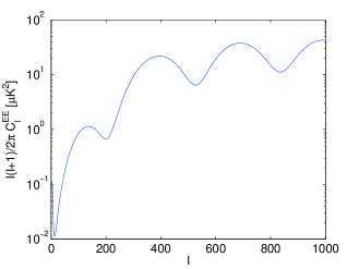
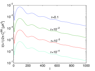
Figure 1: the power spectrum of E (top) and B (bottom): no lensing, B mode power spectrum is plotted for various tensor-to-scalar ratio r𝑟r.

For a Gaussian seed fluctuation model, decomposition coefficients of E and B mode satisfy the following statistical properties:

aE,lmaE,lmdelimited-⟨⟩subscriptsuperscript𝑎𝐸𝑙𝑚subscript𝑎𝐸superscript𝑙superscript𝑚\displaystyle\langle a^{*}_{E,lm}a_{E,l^{\prime}m^{\prime}}\rangle =\displaystyle= ClEEδllδmm,subscriptsuperscript𝐶𝐸𝐸𝑙subscript𝛿𝑙superscript𝑙subscript𝛿𝑚superscript𝑚\displaystyle C^{EE}_{l}\,\delta_{ll^{\prime}}\delta_{mm^{\prime}}, (8)
aB,lmaB,lmdelimited-⟨⟩subscriptsuperscript𝑎𝐵𝑙𝑚subscript𝑎𝐵superscript𝑙superscript𝑚\displaystyle\langle a^{*}_{B,lm}a_{B,l^{\prime}m^{\prime}}\rangle =\displaystyle= ClBBδllδmm,subscriptsuperscript𝐶𝐵𝐵𝑙subscript𝛿𝑙superscript𝑙subscript𝛿𝑚superscript𝑚\displaystyle C^{BB}_{l}\,\delta_{ll^{\prime}}\delta_{mm^{\prime}}, (9)

where delimited-⟨⟩\langle\ldots\rangle denotes an ensemble average. In Fig. 1, we show unlensed ClEEsubscriptsuperscript𝐶𝐸𝐸𝑙C^{EE}_{l} and ClBBsubscriptsuperscript𝐶𝐵𝐵𝑙C^{BB}_{l} of the WMAP concordance ΛΛ\LambdaCDM model for various tensor-to-scalar ratio r𝑟r.

3 E/B decomposition in pixel space

In this section, we are going to derive a pixel-space analogue of E/B decomposition. Using Eq. 3, 6 and 7, we may easily show Eq. 4 and 5 are equivalently given by:

E(𝐧^)𝐸^𝐧\displaystyle E(\mathbf{\hat{n}}) =\displaystyle= (l+2)!(l2)!aE,lmYlm(𝐧^)𝑙2𝑙2subscript𝑎𝐸𝑙𝑚subscript𝑌𝑙𝑚^𝐧\displaystyle\sum\sqrt{\frac{(l+2)!}{(l-2)!}}a_{E,lm}\,Y_{lm}(\mathbf{\hat{n}}) (10)
=\displaystyle= (l+2)!(l2)!aE,lmYlm(𝐧^),𝑙2𝑙2subscriptsuperscript𝑎𝐸𝑙𝑚subscriptsuperscript𝑌𝑙𝑚^𝐧\displaystyle\sum\sqrt{\frac{(l+2)!}{(l-2)!}}a^{*}_{E,lm}\,Y^{*}_{lm}(\mathbf{\hat{n}}),
=\displaystyle= 12(F+(𝐧^,𝐧^)[Q(𝐧^)iU(𝐧^)]dΩ\displaystyle-\frac{1}{2}\left(\int F_{+}(\mathbf{\hat{n}^{\prime}},\mathbf{\hat{n}})\left[Q(\mathbf{\hat{n}^{\prime}})-iU(\mathbf{\hat{n}^{\prime}})\right]\,\mathrm{d}\Omega^{\prime}\right.
+\displaystyle+ F(𝐧^,𝐧^)[Q(𝐧^)+iU(𝐧^)]dΩ),\displaystyle\left.\int F_{-}(\mathbf{\hat{n}^{\prime}},\mathbf{\hat{n}})\left[Q(\mathbf{\hat{n}^{\prime}})+iU(\mathbf{\hat{n}^{\prime}})\right]\,\mathrm{d}\Omega^{\prime}\right),
B(𝐧^)𝐵^𝐧\displaystyle B(\mathbf{\hat{n}}) =\displaystyle= (l+2)!(l2)!aB,lmYlm(𝐧^),𝑙2𝑙2subscript𝑎𝐵𝑙𝑚subscript𝑌𝑙𝑚^𝐧\displaystyle\sum\sqrt{\frac{(l+2)!}{(l-2)!}}a_{B,lm}\,Y_{lm}(\mathbf{\hat{n}}), (11)
=\displaystyle= (l+2)!(l2)!aB,lmYlm(𝐧^),𝑙2𝑙2subscriptsuperscript𝑎𝐵𝑙𝑚subscriptsuperscript𝑌𝑙𝑚^𝐧\displaystyle\sum\sqrt{\frac{(l+2)!}{(l-2)!}}a^{*}_{B,lm}\,Y^{*}_{lm}(\mathbf{\hat{n}}),
=\displaystyle= i2(F+(𝐧^,𝐧^)[Q(𝐧^)iU(𝐧^)]dΩ\displaystyle\frac{i}{2}\left(\int F_{+}(\mathbf{\hat{n}^{\prime}},\mathbf{\hat{n}})\left[Q(\mathbf{\hat{n}^{\prime}})-iU(\mathbf{\hat{n}^{\prime}})\right]\,\mathrm{d}\Omega^{\prime}\right.
\displaystyle- F(𝐧^,𝐧^)[Q(𝐧^)+iU(𝐧^)]dΩ),\displaystyle\left.\int F_{-}(\mathbf{\hat{n}^{\prime}},\mathbf{\hat{n}})\left[Q(\mathbf{\hat{n}^{\prime}})+iU(\mathbf{\hat{n}^{\prime}})\right]\,\mathrm{d}\Omega^{\prime}\right),

where

F±(𝐧^,𝐧^)subscript𝐹plus-or-minussuperscript^𝐧^𝐧\displaystyle F_{\pm}(\mathbf{\hat{n}^{\prime}},\mathbf{\hat{n}}) =\displaystyle= lm(l+2)!(l2)!Ylm±2(𝐧^)Ylm(𝐧^).subscript𝑙𝑚𝑙2𝑙2subscriptsubscript𝑌𝑙𝑚plus-or-minus2superscript^𝐧subscriptsuperscript𝑌𝑙𝑚^𝐧\displaystyle\sum_{lm}\sqrt{\frac{(l+2)!}{(l-2)!}}\;{}_{\pm 2}Y_{lm}(\mathbf{\hat{n}^{\prime}})\;Y^{*}_{lm}(\mathbf{\hat{n}}). (12)

Therefore, we may identify F±(𝐧^,𝐧^)subscript𝐹plus-or-minussuperscript^𝐧^𝐧F_{\pm}(\mathbf{\hat{n}^{\prime}},\mathbf{\hat{n}}) as pixel-space filters for E/B decomposition. Using the property of spin-s𝑠s spherical harmonics Ylms(𝐧^)=Ylms(𝐧^)subscriptsubscriptsuperscript𝑌𝑙𝑚𝑠^𝐧subscriptsubscript𝑌𝑙𝑚𝑠^𝐧{}_{s}Y^{*}_{lm}(\mathbf{\hat{n}})={}_{-s}Y_{l-m}(\mathbf{\hat{n}}), we may show the pair of the filter functions have complex conjugate relation:

F+(𝐧^,𝐧^)=F(𝐧^,𝐧^).subscript𝐹superscript^𝐧^𝐧subscriptsuperscript𝐹superscript^𝐧^𝐧\displaystyle F_{+}(\mathbf{\hat{n}^{\prime}},\mathbf{\hat{n}})=F^{*}_{-}(\mathbf{\hat{n}^{\prime}},\mathbf{\hat{n}}). (13)
Refer to caption
Refer to caption
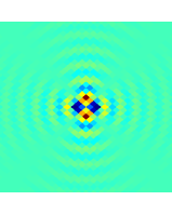
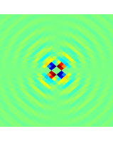
Figure 2: Filter function: Re[F+(𝐧^,𝐧^)]Redelimited-[]subscript𝐹superscript^𝐧^𝐧\mathrm{Re}[F_{+}(\mathbf{\hat{n}^{\prime}},\mathbf{\hat{n}})] (left), Im[F+(𝐧^,𝐧^)]Imdelimited-[]subscript𝐹superscript^𝐧^𝐧\mathrm{Im}[F_{+}(\mathbf{\hat{n}^{\prime}},\mathbf{\hat{n}})] (right) for a fixed 𝐧𝐧\mathbf{n}, and 𝐧superscript𝐧\mathbf{n}^{\prime} spanning 2×2superscript2superscript22^{\circ}\times 2^{\circ} area, F+(𝐧^,𝐧^)=lml1024(l+2)!(l2)!Ylm2(𝐧^)Ylm(𝐧^)subscript𝐹superscript^𝐧^𝐧subscriptsuperscript𝑙1024𝑙𝑚𝑙2𝑙2subscriptsubscript𝑌𝑙𝑚2superscript^𝐧subscriptsuperscript𝑌𝑙𝑚^𝐧F_{+}(\mathbf{\hat{n}^{\prime}},\mathbf{\hat{n}})=\sum^{l\leq 1024}_{lm}\sqrt{\frac{(l+2)!}{(l-2)!}}\;{}_{2}Y_{lm}(\mathbf{\hat{n}^{\prime}})\;Y^{*}_{lm}(\mathbf{\hat{n}})
Refer to caption
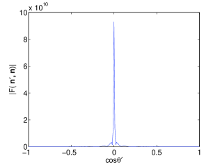
Figure 3: Filter function: modulus |F±(𝐧^,𝐧^)|subscript𝐹plus-or-minussuperscript^𝐧^𝐧|F_{\pm}(\mathbf{\hat{n}^{\prime}},\mathbf{\hat{n}})| for (θ=π/2,ϕ=0)formulae-sequence𝜃𝜋2italic-ϕ0(\theta=\pi/2,\phi=0), highly peaked at cosθ=0superscript𝜃0\cos\theta^{\prime}=0

In Fig. 2, we show the real and imaginary part of F+(𝐧^,𝐧^)subscript𝐹superscript^𝐧^𝐧F_{+}(\mathbf{\hat{n}^{\prime}},\mathbf{\hat{n}}) for a fixed 𝐧𝐧\mathbf{n}. In Fig. 3, we show one dimensional plot of |F±(𝐧^,𝐧^)|subscript𝐹plus-or-minussuperscript^𝐧^𝐧|F_{\pm}(\mathbf{\hat{n}^{\prime}},\mathbf{\hat{n}})| for a fixed 𝐧𝐧\mathbf{n}. As shown in Fig. 2 and 3, our pixel-space filter possesses sharp peaks around 𝐧^^𝐧\mathbf{\hat{n}}. Note that Eq. 12 would approach δ(𝐧^𝐧^)𝛿superscript^𝐧^𝐧\delta(\mathbf{\hat{n}^{\prime}}-\mathbf{\hat{n}}), if (l+2)!(l2)!Ylm±2(𝐧^)𝑙2𝑙2subscriptsubscript𝑌𝑙𝑚plus-or-minus2superscript^𝐧\sqrt{\frac{(l+2)!}{(l-2)!}}\;{}_{\pm 2}Y_{lm}(\mathbf{\hat{n}^{\prime}}) were Ylm(𝐧^)subscript𝑌𝑙𝑚superscript^𝐧Y_{lm}(\mathbf{\hat{n}^{\prime}}). Using Eq. 13, we may easily show Eq. 10 and 11 are equivalently given by:

E(𝐧^)𝐸^𝐧\displaystyle E(\mathbf{\hat{n}}) =\displaystyle= dΩRe[F+(𝐧^,𝐧^)(Q(𝐧^)iU(𝐧^))],differential-dsuperscriptΩRedelimited-[]subscript𝐹superscript^𝐧^𝐧𝑄superscript^𝐧𝑖𝑈superscript^𝐧\displaystyle-\int\mathrm{d}\Omega^{\prime}\,\mathrm{Re}\left[F_{+}(\mathbf{\hat{n}^{\prime}},\mathbf{\hat{n}})\left(Q(\mathbf{\hat{n}^{\prime}})-iU(\mathbf{\hat{n}^{\prime}})\right)\right],
=\displaystyle= dΩRe[F(𝐧^,𝐧^)(Q(𝐧^)+iU(𝐧^))].differential-dsuperscriptΩRedelimited-[]subscript𝐹superscript^𝐧^𝐧𝑄superscript^𝐧𝑖𝑈superscript^𝐧\displaystyle-\int\mathrm{d}\Omega^{\prime}\,\mathrm{Re}\left[F_{-}(\mathbf{\hat{n}^{\prime}},\mathbf{\hat{n}})\left(Q(\mathbf{\hat{n}^{\prime}})+iU(\mathbf{\hat{n}^{\prime}})\right)\right].
B(𝐧^)𝐵^𝐧\displaystyle B(\mathbf{\hat{n}}) =\displaystyle= dΩIm[F+(𝐧^,𝐧^)(Q(𝐧^)iU(𝐧^))],differential-dsuperscriptΩImdelimited-[]subscript𝐹superscript^𝐧^𝐧𝑄superscript^𝐧𝑖𝑈superscript^𝐧\displaystyle-\int\mathrm{d}\Omega^{\prime}\mathrm{Im}\left[F_{+}(\mathbf{\hat{n}^{\prime}},\mathbf{\hat{n}})\left(Q(\mathbf{\hat{n}^{\prime}})-iU(\mathbf{\hat{n}^{\prime}})\right)\right],
=\displaystyle= dΩIm[F(𝐧^,𝐧^)(Q(𝐧^)+iU(𝐧^))].differential-dsuperscriptΩImdelimited-[]subscript𝐹superscript^𝐧^𝐧𝑄superscript^𝐧𝑖𝑈superscript^𝐧\displaystyle\int\mathrm{d}\Omega^{\prime}\mathrm{Im}\left[F_{-}(\mathbf{\hat{n}^{\prime}},\mathbf{\hat{n}})\left(Q(\mathbf{\hat{n}^{\prime}})+iU(\mathbf{\hat{n}^{\prime}})\right)\right].

4 Incomplete sky coverage

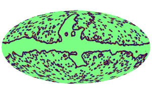
Due to heavy foreground contamination, CMB polarization signal is not estimated reliably over a whole sky. For instance, the WMAP team have subtracted diffuse foregrounds by template-fitting, and masked the regions that cannot be cleaned reliably. In Fig. 7, we show a foreground mask, which combines the WMAP team’s polarization mask with the point source mask and shall be used for our simulation. The E/B decomposition coefficients from a masked sky are given by:

a~E,lmsubscript~𝑎𝐸𝑙𝑚\displaystyle\tilde{a}_{E,lm} =\displaystyle= (a~2,lm+a~2,lm)/2,subscript~𝑎2𝑙𝑚subscript~𝑎2𝑙𝑚2\displaystyle-(\tilde{a}_{2,lm}+\tilde{a}_{-2,lm})/2, (14)
a~B,lmsubscript~𝑎𝐵𝑙𝑚\displaystyle\tilde{a}_{B,lm} =\displaystyle= i(a~2,lma~2,lm)/2,𝑖subscript~𝑎2𝑙𝑚subscript~𝑎2𝑙𝑚2\displaystyle i(\tilde{a}_{2,lm}-\tilde{a}_{-2,lm})/2, (15)

where

a~±2,lm=W(𝐧^)[Q(𝐧^)±iU(𝐧^)]Ylm±2(𝐧^)dΩ.subscript~𝑎plus-or-minus2𝑙𝑚𝑊superscript^𝐧delimited-[]plus-or-minus𝑄^𝐧𝑖𝑈^𝐧subscriptsubscriptsuperscript𝑌𝑙𝑚plus-or-minus2^𝐧differential-dΩ\displaystyle\tilde{a}_{\pm 2,lm}=\int W(\mathbf{\hat{n}^{\prime}})\left[Q(\mathbf{\hat{n}})\pm iU(\mathbf{\hat{n}})\right]\,{}_{\pm 2}Y^{*}_{lm}(\mathbf{\hat{n}})\,\mathrm{d}\Omega. (16)

and W(𝐧^)𝑊superscript^𝐧W(\mathbf{\hat{n}^{\prime}}) is a foreground mask. Therefore, E/B maps reconstructed from incomplete sky are given by:

E~(𝐧^)~𝐸^𝐧\displaystyle\tilde{E}(\mathbf{\hat{n}}) =\displaystyle= (l+2)!(l2)!a~E,lmYlm(𝐧^),𝑙2𝑙2subscript~𝑎𝐸𝑙𝑚subscript𝑌𝑙𝑚^𝐧\displaystyle\sqrt{\frac{(l+2)!}{(l-2)!}}\>\tilde{a}_{E,lm}\,Y_{lm}(\mathbf{\hat{n}}),
=\displaystyle= 12(W(𝐧^)F+(𝐧^,𝐧^)[Q(𝐧^)iU(𝐧^)]dΩ\displaystyle-\frac{1}{2}\left(\int W(\mathbf{\hat{n}^{\prime}})\,F_{+}(\mathbf{\hat{n}^{\prime}},\mathbf{\hat{n}})\left[Q(\mathbf{\hat{n}^{\prime}})-iU(\mathbf{\hat{n}^{\prime}})\right]\,\mathrm{d}\Omega^{\prime}\right.
+\displaystyle+ W(𝐧^)F(𝐧^,𝐧^)[Q(𝐧^)+iU(𝐧^)]dΩ),\displaystyle\left.\int W(\mathbf{\hat{n}^{\prime}})\,F_{-}(\mathbf{\hat{n}^{\prime}},\mathbf{\hat{n}})\left[Q(\mathbf{\hat{n}^{\prime}})+iU(\mathbf{\hat{n}^{\prime}})\right]\,\mathrm{d}\Omega^{\prime}\right),
B~(𝐧^)~𝐵^𝐧\displaystyle\tilde{B}(\mathbf{\hat{n}}) =\displaystyle= (l+2)!(l2)!a~B,lmYlm(𝐧^),𝑙2𝑙2subscript~𝑎𝐵𝑙𝑚subscript𝑌𝑙𝑚^𝐧\displaystyle\sqrt{\frac{(l+2)!}{(l-2)!}}\>\tilde{a}_{B,lm}\,Y_{lm}(\mathbf{\hat{n}}),
=\displaystyle= i2(W(𝐧^)F+(𝐧^,𝐧^)[Q(𝐧^)iU(𝐧^)]dΩ\displaystyle\frac{i}{2}\left(\int W(\mathbf{\hat{n}^{\prime}})\,F_{+}(\mathbf{\hat{n}^{\prime}},\mathbf{\hat{n}})\left[Q(\mathbf{\hat{n}^{\prime}})-iU(\mathbf{\hat{n}^{\prime}})\right]\,\mathrm{d}\Omega^{\prime}\right.
\displaystyle- W(𝐧^)F(𝐧^,𝐧^)[Q(𝐧^)+iU(𝐧^)]dΩ).\displaystyle\left.\int W(\mathbf{\hat{n}^{\prime}})\,F_{-}(\mathbf{\hat{n}^{\prime}},\mathbf{\hat{n}})\left[Q(\mathbf{\hat{n}^{\prime}})+iU(\mathbf{\hat{n}^{\prime}})\right]\,\mathrm{d}\Omega^{\prime}\right).

Since filter functions F±(𝐧^,𝐧^)subscript𝐹plus-or-minussuperscript^𝐧^𝐧F_{\pm}(\mathbf{\hat{n}^{\prime}},\mathbf{\hat{n}}) are sharply peaked around 𝐧^^𝐧\mathbf{\hat{n}}, certain pixels far away from masked regions may contain negligible E/B mixing, and vice versa. Equivalently, E/B mixing is localized in pixels close to the masked regions. For higher pixel resolution, Eq. 12 contains summation up to higher l𝑙l, which makes the peak of the filter function sharper. Therefore, E/B mixing decreases with increase in pixel resolution. The spherical harmonic method (the first line of Eq. 4 and 4) are much faster than the pixel-space method (the second line), while they are mathematically equivalent. Therefore, we are going to rely on spherical harmonic transformation method for our simulation in the next section. However, it should be kept in mind that the pixel-space approach have provided useful insights on E/B decomposition of incomplete sky.

Using Eq. 4, we may show the expected power of B~(𝐧^)~𝐵^𝐧\tilde{B}(\mathbf{\hat{n}}) is given by:

B~2(𝐧^)=14dΩdΩ′′W(𝐧^)W(𝐧^′′)×\displaystyle\langle\tilde{B}^{2}(\mathbf{\hat{n}})\rangle=\frac{1}{4}\int\mathrm{d}\Omega^{\prime}\mathrm{d}\Omega^{\prime\prime}\>W(\mathbf{\hat{n}^{\prime}})W(\mathbf{\hat{n}^{\prime\prime}})\times
(F+(𝐧^,𝐧^)F(𝐧^′′,𝐧^)(Q(𝐧^)iU(𝐧^))(Q(𝐧^′′)+iU(𝐧^′′))\displaystyle(F_{+}(\mathbf{\hat{n}^{\prime}},\mathbf{\hat{n}})F_{-}(\mathbf{\hat{n}^{\prime\prime}},\mathbf{\hat{n}})\langle(Q(\mathbf{\hat{n}^{\prime}})-iU(\mathbf{\hat{n}^{\prime}}))(Q(\mathbf{\hat{n}^{\prime\prime}})+iU(\mathbf{\hat{n}^{\prime\prime}}))\rangle
+F(𝐧^,𝐧^)F+(𝐧^′′,𝐧^)(Q(𝐧^)+iU(𝐧^))(Q(𝐧^′′)iU(𝐧^′′))subscript𝐹superscript^𝐧^𝐧subscript𝐹superscript^𝐧′′^𝐧delimited-⟨⟩𝑄superscript^𝐧𝑖𝑈superscript^𝐧𝑄superscript^𝐧′′𝑖𝑈superscript^𝐧′′\displaystyle+F_{-}(\mathbf{\hat{n}^{\prime}},\mathbf{\hat{n}})F_{+}(\mathbf{\hat{n}^{\prime\prime}},\mathbf{\hat{n}})\langle(Q(\mathbf{\hat{n}^{\prime}})+iU(\mathbf{\hat{n}^{\prime}}))(Q(\mathbf{\hat{n}^{\prime\prime}})-iU(\mathbf{\hat{n}^{\prime\prime}}))\rangle
F+(𝐧^,𝐧^)F+(𝐧^′′,𝐧^)(Q(𝐧^)iU(𝐧^))(Q(𝐧^′′)iU(𝐧^′′))subscript𝐹superscript^𝐧^𝐧subscript𝐹superscript^𝐧′′^𝐧delimited-⟨⟩𝑄superscript^𝐧𝑖𝑈superscript^𝐧𝑄superscript^𝐧′′𝑖𝑈superscript^𝐧′′\displaystyle-F_{+}(\mathbf{\hat{n}^{\prime}},\mathbf{\hat{n}})F_{+}(\mathbf{\hat{n}^{\prime\prime}},\mathbf{\hat{n}})\langle(Q(\mathbf{\hat{n}^{\prime}})-iU(\mathbf{\hat{n}^{\prime}}))(Q(\mathbf{\hat{n}^{\prime\prime}})-iU(\mathbf{\hat{n}^{\prime\prime}}))\rangle\,
F(𝐧^,𝐧^)F(𝐧^′′,𝐧^)(Q(𝐧^)+iU(𝐧^))(Q(𝐧^′′)+iU(𝐧^′′))).\displaystyle-F_{-}(\mathbf{\hat{n}^{\prime}},\mathbf{\hat{n}})F_{-}(\mathbf{\hat{n}^{\prime\prime}},\mathbf{\hat{n}})\langle(Q(\mathbf{\hat{n}^{\prime}})+iU(\mathbf{\hat{n}^{\prime}}))(Q(\mathbf{\hat{n}^{\prime\prime}})+iU(\mathbf{\hat{n}^{\prime\prime}}))\rangle).

where delimited-⟨⟩\langle\ldots\rangle denotes an ensemble average, and

(Q(𝐧^)+iU(𝐧^))(Q(𝐧^′′)+iU(𝐧^′′))delimited-⟨⟩𝑄superscript^𝐧𝑖𝑈superscript^𝐧𝑄superscript^𝐧′′𝑖𝑈superscript^𝐧′′\displaystyle\langle(Q(\mathbf{\hat{n}^{\prime}})+iU(\mathbf{\hat{n}^{\prime}}))(Q(\mathbf{\hat{n}^{\prime\prime}})+iU(\mathbf{\hat{n}^{\prime\prime}}))\rangle
=\displaystyle= l2l+14π(ClEE+ClBB)Yl,22(β,0)e2i(α+γ),subscript𝑙2𝑙14𝜋subscriptsuperscript𝐶𝐸𝐸𝑙subscriptsuperscript𝐶𝐵𝐵𝑙subscriptsubscript𝑌𝑙22𝛽0superscript𝑒2𝑖𝛼𝛾\displaystyle\sum_{l}\sqrt{\frac{2l+1}{4\pi}}(C^{EE}_{l}+C^{BB}_{l})\;{}_{2}Y_{l,-2}(\beta,0)\,e^{2i(\alpha+\gamma)},
(Q(𝐧^)iU(𝐧^))(Q(𝐧^′′)±iU(𝐧^′′))delimited-⟨⟩minus-or-plus𝑄superscript^𝐧𝑖𝑈superscript^𝐧plus-or-minus𝑄superscript^𝐧′′𝑖𝑈superscript^𝐧′′\displaystyle\langle(Q(\mathbf{\hat{n}^{\prime}})\mp iU(\mathbf{\hat{n}^{\prime}}))(Q(\mathbf{\hat{n}^{\prime\prime}})\pm iU(\mathbf{\hat{n}^{\prime\prime}}))\rangle
=\displaystyle= l2l+14π(ClEE+ClBB)Yl,22(β,0)e±2i(αγ),subscript𝑙2𝑙14𝜋subscriptsuperscript𝐶𝐸𝐸𝑙subscriptsuperscript𝐶𝐵𝐵𝑙subscriptsubscript𝑌𝑙22𝛽0superscript𝑒plus-or-minus2𝑖𝛼𝛾\displaystyle\sum_{l}\sqrt{\frac{2l+1}{4\pi}}(C^{EE}_{l}+C^{BB}_{l})\;{}_{2}Y_{l,-2}(\beta,0)\,e^{\pm 2i(\alpha-\gamma)},

and β𝛽\beta is the separation angle between n^superscript^𝑛\hat{n}^{\prime} and n^′′superscript^𝑛′′\hat{n}^{\prime\prime}, α𝛼\alpha and γ𝛾\gamma are the rotation angles respectively, which align e^θsubscript^𝑒𝜃\hat{e}_{\theta} at n^superscript^𝑛\hat{n}^{\prime} and n^′′superscript^𝑛′′\hat{n}^{\prime\prime}with the great circle passing through n^superscript^𝑛\hat{n}^{\prime} and n^′′superscript^𝑛′′\hat{n}^{\prime\prime} (refer to Fig. 1 of Ng & Liu (1999) for a geometrical diagram). Taking into account Eq. 4, 4 and 4, we may easily show that the expected leakage power at 𝐧^^𝐧\mathbf{\hat{n}} is given by

B~E2(𝐧^)=14dΩdΩ′′W(𝐧^)W(𝐧^′′)×\displaystyle\langle\tilde{B}^{2}_{E}(\mathbf{\hat{n}})\rangle=\frac{1}{4}\int\mathrm{d}\Omega^{\prime}\mathrm{d}\Omega^{\prime\prime}\>W(\mathbf{\hat{n}^{\prime}})W(\mathbf{\hat{n}^{\prime\prime}})\times
(F+(𝐧^,𝐧^)F(𝐧^′′,𝐧^)(QE(𝐧^)iUE(𝐧^))(QE(𝐧^′′)+iUE(𝐧^′′))\displaystyle(F_{+}(\mathbf{\hat{n}^{\prime}},\mathbf{\hat{n}})F_{-}(\mathbf{\hat{n}^{\prime\prime}},\mathbf{\hat{n}})\langle(Q_{E}(\mathbf{\hat{n}^{\prime}})-iU_{E}(\mathbf{\hat{n}^{\prime}}))(Q_{E}(\mathbf{\hat{n}^{\prime\prime}})+iU_{E}(\mathbf{\hat{n}^{\prime\prime}}))\rangle
+F(𝐧^,𝐧^)F+(𝐧^′′,𝐧^)(QE(𝐧^)+iUE(𝐧^))(QE(𝐧^′′)iUE(𝐧^′′))subscript𝐹superscript^𝐧^𝐧subscript𝐹superscript^𝐧′′^𝐧delimited-⟨⟩subscript𝑄𝐸superscript^𝐧𝑖subscript𝑈𝐸superscript^𝐧subscript𝑄𝐸superscript^𝐧′′𝑖subscript𝑈𝐸superscript^𝐧′′\displaystyle+F_{-}(\mathbf{\hat{n}^{\prime}},\mathbf{\hat{n}})F_{+}(\mathbf{\hat{n}^{\prime\prime}},\mathbf{\hat{n}})\langle(Q_{E}(\mathbf{\hat{n}^{\prime}})+iU_{E}(\mathbf{\hat{n}^{\prime}}))(Q_{E}(\mathbf{\hat{n}^{\prime\prime}})-iU_{E}(\mathbf{\hat{n}^{\prime\prime}}))\rangle
F+(𝐧^,𝐧^)F+(𝐧^′′,𝐧^)(QE(𝐧^)iUE(𝐧^))(QE(𝐧^′′)iUE(𝐧^′′))subscript𝐹superscript^𝐧^𝐧subscript𝐹superscript^𝐧′′^𝐧delimited-⟨⟩subscript𝑄𝐸superscript^𝐧𝑖subscript𝑈𝐸superscript^𝐧subscript𝑄𝐸superscript^𝐧′′𝑖subscript𝑈𝐸superscript^𝐧′′\displaystyle-F_{+}(\mathbf{\hat{n}^{\prime}},\mathbf{\hat{n}})F_{+}(\mathbf{\hat{n}^{\prime\prime}},\mathbf{\hat{n}})\langle(Q_{E}(\mathbf{\hat{n}^{\prime}})-iU_{E}(\mathbf{\hat{n}^{\prime}}))(Q_{E}(\mathbf{\hat{n}^{\prime\prime}})-iU_{E}(\mathbf{\hat{n}^{\prime\prime}}))\rangle\,
F(𝐧^,𝐧^)F(𝐧^′′,𝐧^)(QE(𝐧^)+iUE(𝐧^))(QE(𝐧^′′)+iUE(𝐧^′′))).\displaystyle-F_{-}(\mathbf{\hat{n}^{\prime}},\mathbf{\hat{n}})F_{-}(\mathbf{\hat{n}^{\prime\prime}},\mathbf{\hat{n}})\langle(Q_{E}(\mathbf{\hat{n}^{\prime}})+iU_{E}(\mathbf{\hat{n}^{\prime}}))(Q_{E}(\mathbf{\hat{n}^{\prime\prime}})+iU_{E}(\mathbf{\hat{n}^{\prime\prime}}))\rangle).

where

(QE(𝐧^)+iUE(𝐧^))(QE(𝐧^′′)+iUE(𝐧^′′))delimited-⟨⟩subscript𝑄𝐸superscript^𝐧𝑖subscript𝑈𝐸superscript^𝐧subscript𝑄𝐸superscript^𝐧′′𝑖subscript𝑈𝐸superscript^𝐧′′\displaystyle\langle(Q_{E}(\mathbf{\hat{n}^{\prime}})+iU_{E}(\mathbf{\hat{n}^{\prime}}))(Q_{E}(\mathbf{\hat{n}^{\prime\prime}})+iU_{E}(\mathbf{\hat{n}^{\prime\prime}}))\rangle
=\displaystyle= l2l+14πClEEYl,22(β,0)e2i(α+γ),subscript𝑙2𝑙14𝜋subscriptsuperscript𝐶𝐸𝐸𝑙subscriptsubscript𝑌𝑙22𝛽0superscript𝑒2𝑖𝛼𝛾\displaystyle\sum_{l}\sqrt{\frac{2l+1}{4\pi}}C^{EE}_{l}\;{}_{2}Y_{l,-2}(\beta,0)\,e^{2i(\alpha+\gamma)},
(QE(𝐧^)iUE(𝐧^))(QE(𝐧^′′)±iUE(𝐧^′′))delimited-⟨⟩minus-or-plussubscript𝑄𝐸superscript^𝐧𝑖subscript𝑈𝐸superscript^𝐧plus-or-minussubscript𝑄𝐸superscript^𝐧′′𝑖subscript𝑈𝐸superscript^𝐧′′\displaystyle\langle(Q_{E}(\mathbf{\hat{n}^{\prime}})\mp iU_{E}(\mathbf{\hat{n}^{\prime}}))(Q_{E}(\mathbf{\hat{n}^{\prime\prime}})\pm iU_{E}(\mathbf{\hat{n}^{\prime\prime}}))\rangle
=\displaystyle= l2l+14πClEEYl,22(β,0)e±2i(αγ).subscript𝑙2𝑙14𝜋subscriptsuperscript𝐶𝐸𝐸𝑙subscriptsubscript𝑌𝑙22𝛽0superscript𝑒plus-or-minus2𝑖𝛼𝛾\displaystyle\sum_{l}\sqrt{\frac{2l+1}{4\pi}}C^{EE}_{l}\;{}_{2}Y_{l,-2}(\beta,0)\,e^{\pm 2i(\alpha-\gamma)}.

Therefore, we may diagnose ambiguous pixels (i.e heavy E/B mixing) by comparing B~E2(𝐧^)delimited-⟨⟩subscriptsuperscript~𝐵2𝐸^𝐧\langle\tilde{B}^{2}_{E}(\mathbf{\hat{n}})\rangle with B~B2(𝐧^)delimited-⟨⟩subscriptsuperscript~𝐵2𝐵^𝐧\langle\tilde{B}^{2}_{B}(\mathbf{\hat{n}})\rangle, where B~B2(𝐧^)delimited-⟨⟩subscriptsuperscript~𝐵2𝐵^𝐧\langle\tilde{B}^{2}_{B}(\mathbf{\hat{n}})\rangle is the local power contributed by B mode and given by replacing ‘E’ with ‘B’ in Eq. 4, 4 and 4. However, estimating Eq. 4, 4 and 4 is prohibitively complicated. Therefore, we are going to resort to Monte-Carlo simulations in order to estimate B~E2(𝐧^)/B~B2(𝐧^)delimited-⟨⟩subscriptsuperscript~𝐵2𝐸^𝐧delimited-⟨⟩subscriptsuperscript~𝐵2𝐵^𝐧\langle\tilde{B}^{2}_{E}(\mathbf{\hat{n}})\rangle/\langle\tilde{B}^{2}_{B}(\mathbf{\hat{n}})\rangle. Depending B~E2(𝐧^)/B~B2(𝐧^)delimited-⟨⟩subscriptsuperscript~𝐵2𝐸^𝐧delimited-⟨⟩subscriptsuperscript~𝐵2𝐵^𝐧\langle\tilde{B}^{2}_{E}(\mathbf{\hat{n}})\rangle/\langle\tilde{B}^{2}_{B}(\mathbf{\hat{n}})\rangle, we may classify the pixel at 𝐧^^𝐧\mathbf{\hat{n}} as ‘pure’ and ‘ambiguous’. To be specific, we may retain pixels satisfying:

B~E2(𝐧^)B~B2(𝐧^)<rcr,delimited-⟨⟩subscriptsuperscript~𝐵2𝐸^𝐧delimited-⟨⟩subscriptsuperscript~𝐵2𝐵^𝐧subscript𝑟𝑐𝑟\displaystyle\frac{\langle\tilde{B}^{2}_{E}(\mathbf{\hat{n}})\rangle}{\langle\tilde{B}^{2}_{B}(\mathbf{\hat{n}})\rangle}<\frac{r_{c}}{r}, (25)

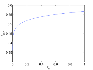
where r𝑟r is the assumed tensor-to-scalar ratio of Monte-Carlo simulation, from which B~E2(𝐧^)/B~B2(𝐧^)delimited-⟨⟩subscriptsuperscript~𝐵2𝐸^𝐧delimited-⟨⟩subscriptsuperscript~𝐵2𝐵^𝐧\langle\tilde{B}^{2}_{E}(\mathbf{\hat{n}})\rangle/\langle\tilde{B}^{2}_{B}(\mathbf{\hat{n}})\rangle is estimated. Therefore, the level of leakage in retained pixels is comparable to the primordial B mode power spectrum of tensor-to-scalar ratio rcsubscript𝑟𝑐r_{c}. In Fig. 4, we show the sky fraction for various rcsubscript𝑟𝑐r_{c}, given a foreground mask shown in Fig. 7. Since sky fraction decreases with lower rcsubscript𝑟𝑐r_{c}, we may not simply set rcsubscript𝑟𝑐r_{c} to a lowest value.

Refer to caption
Figure 4: effective sky fraction fskysubscript𝑓skyf_{\mathrm{sky}} for various cut level rcsubscript𝑟𝑐r_{c}

Therefore, we need to derive an optimal rcsubscript𝑟𝑐r_{c}, which minimizes the estimation error. The estimation error of B mode power spectrum is given by:

ΔClBBΔsubscriptsuperscript𝐶𝐵𝐵𝑙\displaystyle\Delta C^{BB}_{l} =\displaystyle= 2(2l+1)fsky(ClBB+C~lEE+Nl),22𝑙1subscript𝑓skysubscriptsuperscript𝐶𝐵𝐵𝑙subscriptsuperscript~𝐶𝐸𝐸𝑙subscript𝑁𝑙\displaystyle\frac{2}{(2l+1)f_{\mathrm{sky}}}(C^{BB}_{l}+\tilde{C}^{EE}_{l}+N_{l}), (26)
\displaystyle\approx 2(2l+1)fsky(ClBB+rcrClBB+Nl),22𝑙1subscript𝑓skysubscriptsuperscript𝐶𝐵𝐵𝑙subscript𝑟𝑐𝑟subscriptsuperscript𝐶𝐵𝐵𝑙subscript𝑁𝑙\displaystyle\frac{2}{(2l+1)f_{\mathrm{sky}}}(C^{BB}_{l}+\frac{r_{c}}{r}\,C^{BB}_{l}+N_{l}),

where Nlsubscript𝑁𝑙N_{l} is noise power spectrum. Note that the leakage does not bias the B mode power spectrum estimation, but increases the variance, when the power spectrum estimation is made by a pseudo-Clsubscript𝐶𝑙C_{l} method and leakage is taken care of (Hivon et al., 2002a; Grain et al., 2009). By requiring ΔClBB/rc=0Δsubscriptsuperscript𝐶𝐵𝐵𝑙subscript𝑟𝑐0\partial\,\Delta C^{BB}_{l}/\partial r_{c}=0, we get

lnfskyrc=1r+rc+Nl/ClBB(r=1).subscript𝑓skysubscript𝑟𝑐1𝑟subscript𝑟𝑐subscript𝑁𝑙subscriptsuperscript𝐶𝐵𝐵𝑙𝑟1\displaystyle\frac{\partial\ln f_{\mathrm{sky}}}{\partial r_{c}}=\frac{1}{r+r_{c}+N_{l}/C^{BB}_{l}(r=1)}. (27)

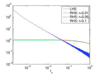
In Fig. 5, we plot the left and right hand side of Eq. 27 for the noise level of Planck HFI instrument, and the multipole l=86𝑙86l=86, which is the peak multipole of primordial B mode power spectrum. From Fig. 5, we find curves intersect at rc4×102subscript𝑟𝑐4superscript102r_{c}\approx 4\times 10^{-2} with weak dependence on r𝑟r. It should be noted that the weak dependence is due to the low signal-to-noise ratio of the considered experiment (i.e. Nl/ClBB(r=1)0much-greater-thansubscript𝑁𝑙subscriptsuperscript𝐶𝐵𝐵𝑙𝑟10N_{l}/C^{BB}_{l}(r=1)\gg 0), and the dependence on r𝑟r is not weak in general. We are going to use rc4×102subscript𝑟𝑐4superscript102r_{c}\approx 4\times 10^{-2} for the simulation in the next section.
Refer to caption
Figure 5: Numerical solution of Eq. 27 for various r𝑟r and the noise level of Planck HFI instrument: two plots represent the Left Hand Side (LHS) and Right Hand Side (RHS) of Eq. 27.

5 Application to simulated data

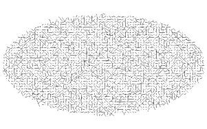
Using the WMAP concordance ΛΛ\LambdaCDM model, we have simulated Stokes parameter Q and U over a whole-sky with a HEALPix pixel resolution (Nside=1024) and 10superscript1010^{\prime} FWHM beam. We have made the inputmap to contain no B mode polarization. Therefore, any non-zero values in output B map are attributed to leakage. We show our simulated polarization map in Fig. 6, where the orientation and length of headless arrows indicates polarization angle and amplitude respectively. Note that the polarization map shows only gradient-like patterns, because they contain only E mode polarization.
Refer to caption
Figure 6: Input polarization map: E mode polarization only
Refer to caption
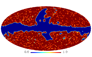
Figure 7: foreground mask: smoothed with 1.5superscript1.51.5^{\circ} FWHM Gaussian kernel.

It is well-known that E/B mixing increases with the length of cut sky boundary (Bunn et al., 2003). We have combined the WMAP team’s polarization mask with the point source mask, and prograded it to Nside=1024. In order to reduce sharp boundaries, we have smoothed the mask with 1.5superscript1.51.5^{\circ} FWHM Gaussian kernel. We have referred to the WMAP team’s boundary smoothing process of Internal Linear Combination map (Hinshaw & et al., 2007). Nevertheless, it should be noted that smoothed boundary is not essential to our method, and further improvement may be possible by using more sophisticated smoothing kernel (Das et al., 2009). In Fig. 7, we show our smoothed mask, whose sky fraction amounts to 0.710.710.71.

Refer to caption
Figure 8: output B~~𝐵\tilde{B} map from incomplete sky

In Fig. 8, we show a B~~𝐵\tilde{B} map, which we have produced from the masked polarization map. Using B~E2(𝐧^)/B~B2(𝐧^)delimited-⟨⟩subscriptsuperscript~𝐵2𝐸^𝐧delimited-⟨⟩subscriptsuperscript~𝐵2𝐵^𝐧\langle\tilde{B}^{2}_{E}(\mathbf{\hat{n}})\rangle/\langle\tilde{B}^{2}_{B}(\mathbf{\hat{n}})\rangle estimated from 103superscript10310^{3} simulation, we have diagnosed ambiguous pixels, and retained pixels of B~E2(𝐧^)/B~B2(𝐧^)<4×102/rdelimited-⟨⟩subscriptsuperscript~𝐵2𝐸^𝐧delimited-⟨⟩subscriptsuperscript~𝐵2𝐵^𝐧4superscript102𝑟\langle\tilde{B}^{2}_{E}(\mathbf{\hat{n}})\rangle/\langle\tilde{B}^{2}_{B}(\mathbf{\hat{n}})\rangle<4\times 10^{-2}/r.

Refer to caption
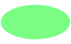
Figure 9: filerted B~~𝐵\tilde{B} map: masked by a foreground mask, and pixels of B~E2(𝐧^)/B~B2(𝐧^)>4×102delimited-⟨⟩subscriptsuperscript~𝐵2𝐸^𝐧delimited-⟨⟩subscriptsuperscript~𝐵2𝐵^𝐧4superscript102\langle\tilde{B}^{2}_{E}(\mathbf{\hat{n}})\rangle/\langle\tilde{B}^{2}_{B}(\mathbf{\hat{n}})\rangle>4\times 10^{-2} are set to zero.
Refer to caption
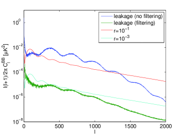
Figure 10: leakage power spectrum and primordial B mode power of various tensor-to-scalar ratio r𝑟r: a blue curve correspond to the leakage power estimated without ambiguous pixel filtering (Fig. 8), a green curve to the leakage power estimated with ambiguous pixel filtering (Fig. 9).

In Fig. 9, we show the B map, where ambiguous pixels are excluded. We find retained pixels of Fig. 9 amount to sky fraction fsky=0.48subscript𝑓sky0.48f_{\mathrm{sky}}=0.48. From the retained pixels, we have estimated the leakage power spectrum by pseudo Clsubscript𝐶𝑙C_{l} method (Wandelt et al., 2001; Hivon et al., 2002b). Power spectrum is usually estimated by a pseudo Clsubscript𝐶𝑙C_{l} method at high multipoles (l>30𝑙30l>30), while by maximum likelihood method or Gibbs sampling at low multipoles (l30𝑙30l\leq 30) (Bond et al., 1998; Eriksen et al., 2004; Hinshaw & et al., 2007; Efstathiou, 2006). However, we find pseudo Clsubscript𝐶𝑙C_{l} method at low multipoles is good enough for our need, since we do not intend accurate estimation of likelihood function. Besides that, we are mainly interested in leakage power at (l>30𝑙30l>30), because primordial B mode power spectrum has a peak around multipoles l90similar-to𝑙90l\sim 90 (see Fig. 1). In Fig. 10, we show the leakage power spectrum and B mode power spectrum of various tensor-to-scalar ratio r𝑟r. Fig. 10 shows leakage power (green) is smaller than B mode power spectrum of r=103𝑟superscript103r=10^{-3} at wide range of multipoles (50l2000less-than-or-similar-to50𝑙less-than-or-similar-to200050\la l\la 2000), when ambiguous pixels are excluded (i.e. the B map in Fig. 9). In Fig. 10, we also show the leakage power (blue) estimated without filtering (i.e. the B map in Fig. 8). Obviously, we have reduced leakage significantly by excluding ambiguous pixels.

6 scale-dependence of leakage

In order to reduce leakage, we have removed ambiguous pixels in a scale-independent way. On the other hand, it is known that leakage has some dependence on scales as well as real-space. Specifically, leakage of low l𝑙l extends over large area, while leakage of high l𝑙l is often confined to the small area nearby the boundary. Therefore, one may argue that our method does not reduce the leakage at low l𝑙l as effectively as that of high l𝑙l or leads to unnecessary loss of information. However, as shown in Fig. 8, leakage is relatively localized in pixel space, and we were able to reduced leakage very significantly at wide range of multipoles, while retaining sky fraction 0.480.480.48. Besides that, our simulation shows the leakage at lowest l𝑙l is reduced significantly as well. It is also possible to implement a further leakage reduction in a scale-dependent way, after ambiguous pixels are removed. Nevertheless, a hybrid method, which exploits scale and position dependence simultaneously, may be most optimal. A wavelet approach may be promising for such implementation, since wavelet functions are, in general, well-localized in harmonic space as well as pixel space. We defer a rigorous investigation to a separate publication.

7 Discussion

We have investigated E/B decomposition in pixel space, and shown that we may produce E/B decomposed maps by convolving polarization maps with certain filter functions of a sharp peak. We find that E/B mixing due to incomplete sky is localized in pixel-space, and negligible in the regions far away from masked area. By estimating the expected local leakage power and comparing it with the expected pure mode power, we have diagnosed ambiguous pixels and excluded them. Our criteria for ambiguous pixels (i.e. rcsubscript𝑟𝑐r_{c}) is associated with the tensor-to-scalar ratio of B mode power spectrum, which the leakage power is comparable to. The estimation error ΔClΔsubscript𝐶𝑙\Delta C_{l} may increases with lower rcsubscript𝑟𝑐r_{c}, because sky fraction decreases. Therefore, we have solved ΔCl/rc=0Δsubscript𝐶𝑙subscript𝑟𝑐0\partial\Delta C_{l}/\partial r_{c}=0 and obtained the optimal rcsubscript𝑟𝑐r_{c}, which minimizes the estimation error, given a foreground mask and noise level. We have applied our method to simulated maps blocked by a foreground mask. Simulation shows that leakage power is subdominant in comparison with unlensed B mode power spectrum of r1×103similar-to𝑟1superscript103r\sim 1\times 10^{-3} at wide range of multipoles (50l2000less-than-or-similar-to50𝑙less-than-or-similar-to200050\la l\la 2000), while pixels of sky fraction 0.480.480.48 are retained. We may apply our method equally to small sky patch observation, by treating unobserved sky as masked region. From simulation with sky patch of simple symmetric shape, we have confirmed our method reduce E/B mixing very effectively. A rigorous investigation is deferred to a separate publication.

Noise is slightly correlated from pixel to pixel in E and B maps, even when interpixel correlation is absent in Q and U maps. However, this interpixel noise correlation induced by E/B decomposition is not confined to our method, but E/B decomposition in general. Besides that, we find interpixel noise correlation may be neglected without sacrificing the accuracy of error analysis (refer to Appendix A for details). Therefore, it does not limit the applicability of our method.

Current observations such as WMAP were unable to detect B mode polarization. Therefore, we did not attempt to apply our method to observation data. When Planck polarization data of high Signal-to-Noise-Ratio (SNR) are available in near future, we may apply our method to the data, and be able to detect B mode polarization.

Acknowledgements.
We are grateful to the anonymous referee for thorough reading and helpful comments, which leads to significant improvement of this work. We acknowledge the use of the Legacy Archive for Microwave Background Data Analysis (LAMBDA) and the HEALPix package (Gorski et al., 1999, 2005). This work is supported by FNU grant 272-06-0417, 272-07-0528 and 21-04-0355. This work is supported in part by Danmarks Grundforskningsfond, which allowed the establishment of the Danish Discovery Center.

Appendix A error analysis

Power spectrum is usually estimated by pseudo-Clsubscript𝐶𝑙C_{l} method at high multipoles (Wandelt et al., 2001; Hivon et al., 2002b; Efstathiou, 2006; Nolta & et al., 2008; Larson et al., 2010). According to pseudo-Clsubscript𝐶𝑙C_{l} method, we may estimate power spectrum as follows (Wandelt et al., 2001; Hivon et al., 2002b):

C^lBB=l(𝐌1)llC~lBB.subscriptsuperscript^𝐶𝐵𝐵𝑙subscriptsuperscript𝑙subscriptsuperscript𝐌1𝑙superscript𝑙subscriptsuperscript~𝐶𝐵𝐵superscript𝑙\displaystyle\hat{C}^{BB}_{l}=\sum_{l^{\prime}}(\mathbf{M}^{-1})_{ll^{\prime}}\tilde{C}^{BB}_{l^{\prime}}. (28)

where

𝐌ll=2l+14πl′′m′′|wl′′m′′|2{(lll′′202)(lll′′202)}2,subscript𝐌𝑙superscript𝑙2superscript𝑙14𝜋subscriptsuperscript𝑙′′superscript𝑚′′superscriptsubscript𝑤superscript𝑙′′superscript𝑚′′2superscript𝑙superscript𝑙superscript𝑙′′202𝑙superscript𝑙superscript𝑙′′2022\displaystyle\mathbf{M}_{ll^{\prime}}=\frac{2l^{\prime}+1}{4\pi}\sum_{l^{\prime\prime}m^{\prime\prime}}|w_{l^{\prime\prime}m^{\prime\prime}}|^{2}\left\{\left(\begin{array}[]{ccc}l&l^{\prime}&l^{\prime\prime}\\ 2&0&-2\end{array}\right)-\left(\begin{array}[]{ccc}l&l^{\prime}&l^{\prime\prime}\\ -2&0&2\end{array}\right)\right\}^{2}, (33)

and

wl′′m′′=dΩW(𝐧^)Yl′′m′′(𝐧^),subscript𝑤superscript𝑙′′superscript𝑚′′differential-dΩ𝑊^𝐧subscriptsuperscript𝑌superscript𝑙′′superscript𝑚′′^𝐧\displaystyle w_{l^{\prime\prime}m^{\prime\prime}}=\int\mathrm{d}\Omega\,W(\mathbf{\hat{n}})Y^{*}_{l^{\prime\prime}m^{\prime\prime}}(\mathbf{\hat{n}}), (34)

with W(𝐧^)𝑊^𝐧W(\mathbf{\hat{n}}) being a foreground mask function. The pseudo-quantity C~lsubscript~𝐶𝑙\tilde{C}_{l} and a~lmjsubscriptsuperscript~𝑎𝑗𝑙𝑚\tilde{a}^{j}_{lm} are given by:

C~l=12l+1ma~lmj(a~lmk),subscript~𝐶𝑙12𝑙1subscript𝑚subscriptsuperscript~𝑎𝑗𝑙𝑚superscriptsubscriptsuperscript~𝑎𝑘𝑙𝑚\displaystyle\tilde{C}_{l}=\frac{1}{2l+1}\sum_{m}\tilde{a}^{j}_{lm}(\tilde{a}^{k}_{lm})^{*}, (35)
a~lmj=dΩW(𝐧^)Δj(𝐧^)Ylm(𝐧^),subscriptsuperscript~𝑎𝑗𝑙𝑚differential-dΩ𝑊^𝐧superscriptΔ𝑗^𝐧subscriptsuperscript𝑌𝑙𝑚^𝐧\displaystyle\tilde{a}^{j}_{lm}=\int\mathrm{d}\Omega\,W(\mathbf{\hat{n}})\,\Delta^{j}(\mathbf{\hat{n}})Y^{*}_{lm}(\mathbf{\hat{n}}), (36)

where j𝑗j and k𝑘k refers to a DA-year combination and Δ(𝐧^)Δ^𝐧\Delta(\mathbf{\hat{n}}) refers to data (T, E or B). We may split a~lmjsubscriptsuperscript~𝑎𝑗𝑙𝑚\tilde{a}^{j}_{lm} into signal and noise:

a~lmj=a~lm+N~lmj.subscriptsuperscript~𝑎𝑗𝑙𝑚subscript~𝑎𝑙𝑚subscriptsuperscript~𝑁𝑗𝑙𝑚\displaystyle\tilde{a}^{j}_{lm}=\tilde{a}_{lm}+\tilde{N}^{j}_{lm}. (37)

The noise part is given by:

N~lm=4πnpixiNiYlmi,subscript~𝑁𝑙𝑚4𝜋subscript𝑛pixsubscript𝑖subscript𝑁𝑖subscriptsuperscript𝑌𝑖𝑙𝑚\displaystyle\tilde{N}_{lm}=\frac{4\pi}{n_{\mathrm{pix}}}\sum_{i}N_{i}\,Y^{i}_{lm}, (38)

where a pixel index i𝑖i runs over pixels outside a foreground mask, and Nisubscript𝑁𝑖N_{i} refers to noise at i𝑖ith pixel. By central limit theorem (Arfken & Weber, 2000; K. F. Riley M. P. Hobson, 2006), N~lmjsubscriptsuperscript~𝑁𝑗𝑙𝑚\tilde{N}^{j}_{lm} follows a Gaussian distribution, and is uncorrelated among distinct j𝑗jth DA-year data (i.e. N~lmj(N~lmk)δjkproportional-todelimited-⟨⟩subscriptsuperscript~𝑁𝑗𝑙𝑚superscriptsubscriptsuperscript~𝑁𝑘𝑙𝑚subscript𝛿𝑗𝑘\langle\tilde{N}^{j}_{lm}(\tilde{N}^{k}_{lm})^{*}\rangle\propto\delta_{jk}).

If cross power spectra are used (i.e. jk𝑗𝑘j\neq k), noise does not bias estimation, and its statistical properties need to be known only for errors analysis (Hinshaw & et al., 2007). In order to understand the effect of noise on error analysis, let us consider covariance of C^lsubscript^𝐶𝑙\hat{C}_{l}:

Cov(C^l1,C^l2)=C^l1C^l2Cl1Cl2,Covsubscript^𝐶subscript𝑙1subscript^𝐶subscript𝑙2delimited-⟨⟩subscript^𝐶subscript𝑙1subscript^𝐶subscript𝑙2subscript𝐶subscript𝑙1subscript𝐶subscript𝑙2\displaystyle\mathrm{Cov}(\hat{C}_{l_{1}},\hat{C}_{l_{2}})=\langle\hat{C}_{l_{1}}\hat{C}_{l_{2}}\rangle-C_{l_{1}}C_{l_{2}}, (39)

where Clsubscript𝐶𝑙C_{l} is a theoretical power spectrum and

C^l1C^l2delimited-⟨⟩subscript^𝐶subscript𝑙1subscript^𝐶subscript𝑙2\displaystyle\langle\hat{C}_{l_{1}}\hat{C}_{l_{2}}\rangle =\displaystyle= l(𝐌1)l1lC~ll(𝐌1)l2lC~l,delimited-⟨⟩subscript𝑙subscriptsuperscript𝐌1subscript𝑙1𝑙subscript~𝐶𝑙subscriptsuperscript𝑙subscriptsuperscript𝐌1subscript𝑙2superscript𝑙subscript~𝐶superscript𝑙\displaystyle\langle\sum_{l}(\mathbf{M}^{-1})_{l_{1}l}\>\tilde{C}_{l}\sum_{l^{\prime}}(\mathbf{M}^{-1})_{l_{2}l^{\prime}}\>\tilde{C}_{l^{\prime}}\rangle, (40)
=\displaystyle= l(𝐌1)l1ll(𝐌1)l2lC~lC~l.subscript𝑙subscriptsuperscript𝐌1subscript𝑙1𝑙subscriptsuperscript𝑙subscriptsuperscript𝐌1subscript𝑙2superscript𝑙delimited-⟨⟩subscript~𝐶𝑙subscript~𝐶superscript𝑙\displaystyle\sum_{l}(\mathbf{M}^{-1})_{l_{1}l}\sum_{l^{\prime}}(\mathbf{M}^{-1})_{l_{2}l^{\prime}}\langle\tilde{C}_{l}\tilde{C}_{l^{\prime}}\rangle.

Using Eq. 35 and 37, we find

C~lC~l=Adelimited-⟨⟩subscript~𝐶𝑙subscript~𝐶superscript𝑙𝐴\displaystyle\langle\tilde{C}_{l}\tilde{C}_{l^{\prime}}\rangle=A
+\displaystyle+ 1(2l+1)(2l+1)mmN~lmj(N~lmj)N~lmk(N~lmk),12𝑙12superscript𝑙1subscript𝑚superscript𝑚delimited-⟨⟩subscriptsuperscript~𝑁𝑗𝑙𝑚superscriptsubscriptsuperscript~𝑁𝑗superscript𝑙superscript𝑚delimited-⟨⟩subscriptsuperscript~𝑁𝑘𝑙𝑚superscriptsubscriptsuperscript~𝑁𝑘superscript𝑙superscript𝑚\displaystyle\frac{1}{(2l+1)(2l^{\prime}+1)}\sum_{mm^{\prime}}\langle\tilde{N}^{j}_{lm}(\tilde{N}^{j}_{l^{\prime}m^{\prime}})^{*}\rangle\langle\tilde{N}^{k}_{lm}(\tilde{N}^{k}_{l^{\prime}m^{\prime}})^{*}\rangle,

where A𝐴A denotes terms irrelevant to noise. Therefore, we need to estimate noise covariance N~lmj(N~lmj)delimited-⟨⟩subscriptsuperscript~𝑁𝑗𝑙𝑚superscriptsubscriptsuperscript~𝑁𝑗superscript𝑙superscript𝑚\langle\tilde{N}^{j}_{lm}(\tilde{N}^{j}_{l^{\prime}m^{\prime}})^{*}\rangle in order to estimate Eq. A. First, let us consider diagonal elements of noise covariance:

N~lmN~lmdelimited-⟨⟩subscript~𝑁𝑙𝑚subscriptsuperscript~𝑁𝑙𝑚\displaystyle\langle\tilde{N}_{lm}\tilde{N}^{*}_{lm}\rangle
=\displaystyle= 16π2npix2iNi2|Ylmi|2+32π2npix2ii>iNiNiYlmi(Ylmi).16superscript𝜋2subscriptsuperscript𝑛2pixsubscript𝑖delimited-⟨⟩subscriptsuperscript𝑁2𝑖superscriptsubscriptsuperscript𝑌𝑖𝑙𝑚232superscript𝜋2subscriptsuperscript𝑛2pixsubscript𝑖subscriptsuperscript𝑖𝑖delimited-⟨⟩subscript𝑁𝑖subscript𝑁superscript𝑖subscriptsuperscript𝑌𝑖𝑙𝑚superscriptsubscriptsuperscript𝑌superscript𝑖𝑙𝑚\displaystyle\frac{16\pi^{2}}{n^{2}_{\mathrm{pix}}}\sum_{i}\langle N^{2}_{i}\rangle|Y^{i}_{lm}|^{2}+\frac{32\pi^{2}}{n^{2}_{\mathrm{pix}}}\sum_{i}\sum_{i^{\prime}>i}\langle N_{i}N_{i^{\prime}}\rangle Y^{i}_{lm}(Y^{i^{\prime}}_{lm})^{*}.

The main contribution of Eq. A comes from the first term, because of cancellation through summation in the second term. Therefore, we find with good approximation:

N~lmN~lm16π2npix2iNi2|Ylmi|2.delimited-⟨⟩subscript~𝑁𝑙𝑚subscriptsuperscript~𝑁𝑙𝑚16superscript𝜋2subscriptsuperscript𝑛2pixsubscript𝑖delimited-⟨⟩subscriptsuperscript𝑁2𝑖superscriptsubscriptsuperscript𝑌𝑖𝑙𝑚2\displaystyle\langle\tilde{N}_{lm}\tilde{N}^{*}_{lm}\rangle\approx\frac{16\pi^{2}}{n^{2}_{\mathrm{pix}}}\sum_{i}\langle N^{2}_{i}\rangle|Y^{i}_{lm}|^{2}.

Off-diagonal elements of noise covariance are given by:

N~lmN~lmdelimited-⟨⟩subscript~𝑁𝑙𝑚subscriptsuperscript~𝑁superscript𝑙superscript𝑚\displaystyle\langle\tilde{N}_{lm}\tilde{N}^{*}_{l^{\prime}m^{\prime}}\rangle =\displaystyle= 16π2npix2iNi2Ylmi(Ylmi)16superscript𝜋2subscriptsuperscript𝑛2pixsubscript𝑖delimited-⟨⟩subscriptsuperscript𝑁2𝑖subscriptsuperscript𝑌𝑖𝑙𝑚superscriptsubscriptsuperscript𝑌𝑖superscript𝑙superscript𝑚\displaystyle\frac{16\pi^{2}}{n^{2}_{\mathrm{pix}}}\sum_{i}\langle N^{2}_{i}\rangle Y^{i}_{lm}(Y^{i}_{l^{\prime}m^{\prime}})^{*}
+\displaystyle+ 32π2npix2ii>iNiNiYlmi(Ylmi).32superscript𝜋2subscriptsuperscript𝑛2pixsubscript𝑖subscriptsuperscript𝑖𝑖delimited-⟨⟩subscript𝑁𝑖subscript𝑁superscript𝑖subscriptsuperscript𝑌𝑖𝑙𝑚superscriptsubscriptsuperscript𝑌superscript𝑖superscript𝑙superscript𝑚\displaystyle\frac{32\pi^{2}}{n^{2}_{\mathrm{pix}}}\sum_{i}\sum_{i^{\prime}>i}\langle N_{i}N_{i^{\prime}}\rangle Y^{i}_{lm}(Y^{i^{\prime}}_{l^{\prime}m^{\prime}})^{*}.

Comparing A with Eq. A, we may see the magnitude of off-diagonal elements is much smaller than that of diagonal elements, because cancellation through summation arise both in the first and the second term of Eq. A. Therefore, we find noise covariance as follow:

N~lmN~lmδllδmm16π2npix2iNi2|Ylmi|2.delimited-⟨⟩subscript~𝑁𝑙𝑚subscriptsuperscript~𝑁superscript𝑙superscript𝑚subscript𝛿𝑙superscript𝑙subscript𝛿𝑚superscript𝑚16superscript𝜋2subscriptsuperscript𝑛2pixsubscript𝑖delimited-⟨⟩subscriptsuperscript𝑁2𝑖superscriptsubscriptsuperscript𝑌𝑖𝑙𝑚2\displaystyle\langle\tilde{N}_{lm}\tilde{N}^{*}_{l^{\prime}m^{\prime}}\rangle\approx\delta_{ll^{\prime}}\delta_{mm^{\prime}}\frac{16\pi^{2}}{n^{2}_{\mathrm{pix}}}\sum_{i}\langle N^{2}_{i}\rangle|Y^{i}_{lm}|^{2}. (44)

Using Eq. 39, 40, A and 44, we find covariance of C^lsubscript^𝐶𝑙\hat{C}_{l}:

Cov(C^l1,C^l2)C+l(𝐌1)l1l(𝐌1)l2lCovsubscript^𝐶subscript𝑙1subscript^𝐶subscript𝑙2𝐶subscript𝑙subscriptsuperscript𝐌1subscript𝑙1𝑙subscriptsuperscript𝐌1subscript𝑙2𝑙\displaystyle\mathrm{Cov}(\hat{C}_{l_{1}},\hat{C}_{l_{2}})\approx C+\sum_{l}(\mathbf{M}^{-1})_{l_{1}l}(\mathbf{M}^{-1})_{l_{2}l}
×\displaystyle\times 256π4npix4(2l+1)2mii(Nij)2(Nik)2|Ylmi|2|Ylmi|2,256superscript𝜋4subscriptsuperscript𝑛4pixsuperscript2𝑙12subscript𝑚subscript𝑖superscript𝑖delimited-⟨⟩superscriptsubscriptsuperscript𝑁𝑗𝑖2delimited-⟨⟩superscriptsubscriptsuperscript𝑁𝑘superscript𝑖2superscriptsubscriptsuperscript𝑌𝑖𝑙𝑚2superscriptsubscriptsuperscript𝑌superscript𝑖𝑙𝑚2\displaystyle\;\frac{256\pi^{4}}{n^{4}_{\mathrm{pix}}(2l+1)^{2}}\sum_{m}\sum_{ii^{\prime}}\langle(N^{j}_{i})^{2}\rangle\langle(N^{k}_{i^{\prime}})^{2}\rangle|Y^{i}_{lm}|^{2}|Y^{i^{\prime}}_{lm}|^{2},

where C𝐶C denotes terms irrelevant to noise. As shown in Eq. A, we may neglect interpixel noise correlation in computing covariance of C^lsubscript^𝐶𝑙\hat{C}_{l},

References

  • Ade & et al. (2008) Ade, P. & et al. 2008, ApJ, 674, 22
  • Arfken & Weber (2000) Arfken, G. B. & Weber, H. J. 2000, Mathematical Methods for Physicists, 5th edn. (San Diego, CA USA: Academic Press)
  • Bond et al. (1998) Bond, J. R., Jaffe, A. H., & Knox, L. 1998, Phys. Rev. D, 57, 2117
  • Brown & et al. (2009) Brown, M. L. & et al. 2009, ApJ, 705, 978
  • Bunn et al. (2003) Bunn, E. F., Zaldarriaga, M., Tegmark, M., & de Oliveira-Costa, A. 2003, 67, 023501
  • Das et al. (2009) Das, S., Hajian, A., & Spergel, D. N. 2009, Phys. Rev. D, 79, 083008
  • Dodelson (2003) Dodelson, S. 2003, Modern Cosmology, 2nd edn. (Academic Press)
  • Efstathiou (2006) Efstathiou, G. 2006, MNRAS, 370, 343
  • Eriksen et al. (2004) Eriksen, H. K., O’Dwyer, I. J., Jewell, J. B., et al. 2004, ApJ, 155, 227
  • Gorski et al. (2005) Gorski, K. M., Hivon, E., Banday, A. J., et al. 2005, ApJ, 622, 759
  • Gorski et al. (1999) Gorski, K. M., Wandelt, B. D., Hansen, F. K., Hivon, E., & Banday, A. J. 1999, ArXiv Astrophysics e-prints
  • Grain et al. (2009) Grain, J., Tristram, M., & Stompor, R. 2009, Phys. Rev. D, 79, 123515
  • Halverson et al. (2002) Halverson, N. W., Leitch, E. M., Pryke, C., et al. 2002, ApJ, 568, 38
  • Hinderks & et al. (2008) Hinderks, J. & et al. 2008, ArXiv e-prints
  • Hinshaw & et al. (2007) Hinshaw, G. & et al. 2007, ApJ, 170, 288
  • Hivon et al. (2002a) Hivon, E., Górski, K. M., Netterfield, C. B., et al. 2002a, ApJ, 567, 2
  • Hivon et al. (2002b) Hivon, E., Górski, K. M., Netterfield, C. B., et al. 2002b, ApJ, 567, 2
  • K. F. Riley M. P. Hobson (2006) K. F. Riley M. P. Hobson, S. J. B. 2006, Mathematical Methods for Physics and Engineering: A Comprehensive Guide, 3rd edn. (Cambridge University Press)
  • Kamionkowski et al. (1997) Kamionkowski, M., Kosowsky, A., & Stebbins, A. 1997, Phys. Rev. D, 55, 7368
  • Kim (2007a) Kim, J. 2007a, MNRAS, 375, 625
  • Kim (2007b) Kim, J. 2007b, MNRAS, 375, 615
  • Komatsu et al. (2010) Komatsu, E., Smith, K. M., Dunkley, J., et al. 2010, ArXiv e-prints
  • Kovac et al. (2002) Kovac, J., Leitch, E. M., Pryke, C., et al. 2002, Nature, 420, 772
  • Kraus (1986) Kraus, J. 1986, Radio Astronomy, 2nd edn. (Powell, Ohio USA: Cygnus-Quasar Books)
  • Larson et al. (2010) Larson, D., Dunkley, J., Hinshaw, G., et al. 2010
  • Leitch et al. (2005) Leitch, E. M., Kovac, J. M., Halverson, N. W., et al. 2005, ApJ, 624, 10
  • Leitch et al. (2002) Leitch, E. M., Kovac, J. M., Pryke, C., et al. 2002, Nature, 420, 763
  • Lewis (2003) Lewis, A. 2003, Phys. Rev. D, 68, 083509
  • Lewis et al. (2002) Lewis, A., Challinor, A., & Turok, N. 2002, Phys. Rev. D, 65, 023505
  • Liddle & Lyth (2000) Liddle, A. R. & Lyth, D. H. 2000, Cosmological Inflation and Large-Scale Structure, 1st edn. (Cambridge University Press)
  • Mukhanov (2005) Mukhanov, V. 2005, Physical Foundations of Cosmology, 1st edn. (Cambridge University Press)
  • Ng & Liu (1999) Ng, K. & Liu, G. 1999, International Journal of Modern Physics D, 8, 61
  • Nolta & et al. (2008) Nolta, M. R. & et al. 2008, submitted to ApJ, arXiv:0803.0593
  • Pryke & et al. (2009) Pryke, C. & et al. 2009, ApJ, 692, 1247
  • Pryke et al. (2002a) Pryke, C., Halverson, N. W., Kovac, J. M., et al. 2002a, ApJ, 568, 28
  • Pryke et al. (2002b) Pryke, C., Halverson, N. W., Leitch, E. M., et al. 2002b, ApJ, 568, 46
  • Rohlfs & Wilson (2003) Rohlfs, K. & Wilson, T. L. 2003, Tools of Radio Astronomy, 4th edn. (New York, NY USA: Springer-Verlag)
  • Seljak & Hirata (2004) Seljak, U. & Hirata, C. M. 2004, Phys. Rev. D, 69, 043005
  • Smith (2006) Smith, K. M. 2006, Phys. Rev. D, 74, 083002
  • The Planck Collaboration (2006) The Planck Collaboration. 2006, ArXiv Astrophysics e-prints
  • Tucci et al. (2005) Tucci, M., Martínez-González, E., Vielva, P., & Delabrouille, J. 2005, MNRAS, 360, 935
  • Wandelt et al. (2001) Wandelt, B. D., Hivon, E., & Górski, K. M. 2001, Phys. Rev. D, 64, 083003
  • Zaldarriaga (1998) Zaldarriaga, M. 1998, ApJ, 503, 1
  • Zaldarriaga & Seljak (1997) Zaldarriaga, M. & Seljak, U. 1997, Phys. Rev. D, 55, 1830