Nearly Optimal Resource Allocation for Downlink OFDMA in 2-D Cellular Networks

Abstract

In this paper, we propose a resource allocation algorithm for the downlink of sectorized two-dimensional (2-D) OFDMA cellular networks assuming statistical Channel State Information (CSI) and fractional frequency reuse. The proposed algorithm can be implemented in a distributed fashion without the need to any central controlling units. Its performance is analyzed assuming fast fading Rayleigh channels and Gaussian distributed multicell interference. We show that the transmit power of this simple algorithm tends, as the number of users grows to infinity, to the same limit as the minimal power required to satisfy all users’ rate requirements i.e., the proposed resource allocation algorithm is asymptotically optimal. As a byproduct of this asymptotic analysis, we characterize a relevant value of the reuse factor that only depends on an average state of the network.

I Introduction

We address in this work the problem of resource allocation (power control and subcarrier assignment) for the downlink of sectorized OFDMA networks impaired with multicell interference. A considerable research interest has been lately dedicated to this problem since the adoption of OFDMA in a number of current and future wireless standards such as WiMax and 3GPP-LTE. In principle, the problem of resource allocation should be jointly solved in all the cells of the system. In most of the practical situations, this optimization problem is difficult to solve. Therefore, most of the related works in the literature focus on the single cell case (e.g., [1]-[6]). Fewer works address the more involved multicell allocation problem. In this context, we cite [7]-[11] in the case of perfect CSI at the transmitters side, and [12, 13] in the case of imperfect CSI. In [12, 13], all the available subcarriers are likely to be used by different base stations and are thus subject to multicell interference. In such a configuration, interference may reach excessive levels, especially for users located at cells borders.

Similarly to [12, 13], we assume in this paper that users’ channels undergo fast fading and that the CSI at the base stations is limited to some channel statistics. However, contrary to these two works, we consider that a certain subset of subcarriers is shared orthogonally between the adjacent base stations (and is thus “protected” from multicell interference) while the remaining subcarriers are “non protected” since they are reused by different base stations. This so-called fractional frequency reuse (or FFR) is recommended in a number of standards e.g., in [14] for IEEE 802.16 (WiMax) [15], as a way to avoid severe inter-cell interference. The ratio between the number of non protected subcarriers and the total number of subcarriers is generally referred to as the reuse factor and is denoted in the sequel by $\alpha$.

Few works in the literature (we cite [16, 17, 18] without being exclusive) have addressed the problem of resource allocation for FFR-based OFDMA networks, and none of them fits into the above framework which is considered in this paper. The particular problem considered in [16] consists in maximizing a system-wide utility function under a power constraint. In this context, the authors propose a distributed iterative allocation algorithm that is based on estimating the level of multicell interference rather than computing it. Of course, resource allocation schemes that do not resort to such simplifications are highly preferable. In the same context, authors of [17] consider the problem of minimizing the total transmit power needed to satisfy all users’ rate requirements. For that sake, they propose a heuristic allocation algorithm without any assessment of its deviation from the optimal solution to the latter problem. Moreover, the selection of a relevant reuse factor is not addressed. Finally, authors of [18] assume that subcarrier assignment is done separately and in advance. The major drawback of this work is thus that joint power control and subcarrier assignment is not addressed.

In our work, we investigate the problem of power control and subcarrier assignment for the downlink of FFR-based OFDMA systems allowing to satisfy all users’ rate requirements while spending the least possible power at the transmitters’ side. In our previous work [19, 20], the solution to this problem is characterized in the special case of one-dimensional (1-D) cellular networks where all users and base stations are located on a line. Unfortunately, it is much more difficult to characterize this solution in the case of 2-D networks. In the present work, our aim is to propose a suboptimal resource allocation strategy for these 2-D networks and to study its performance with respect to the above optimization problem. Our allocation algorithm assumes that users of each cell are divided prior to resource allocation into two groups separated by a fixed curve. The first group is composed of closer users to the base station. These users are constrained to modulate non protected subcarriers and are thus subject to multicell interference. The second group comprises the farthest users who are constrained to modulate interference-free subcarriers. In order to relevantly select the aforementioned separating curves, we study the limit of an optimal solution to the resource allocation problem as the number of users grows to infinity. We show that if the curves are set using the results of this asymptotic analysis, then the limit of the transmit power of the proposed suboptimal algorithm is equal to the limit of the transmit power of the optimal resource allocation. As a byproduct, we are able to determine a relevant value of the reuse factor. Indeed, the asymptotic transmit power depends on the average rate requirement and on the density of users in each cell. It also depends on the value $\alpha$ of the frequency reuse factor. We can therefore define the optimal reuse factor as the value of $\alpha$ which minimizes this asymptotic power. The main contributions of this work are thus the following.

1. A practical resource allocation algorithm that can be implemented in a distributed manner is proposed for the downlink of a sectorized OFDMA network assuming fractional frequency reuse and statistical CSI. The transmit power of this simple algorithm tends, as the number of users grows to infinity, to the same limit as the minimal power required to satisfy all users’ rate requirements.

2. As a byproduct of our study of the above algorithm, we prove that the simple scheme consisting in separating users of each cell beforehand into interference-free users (constrained to modulate only non reusable subcarriers) and interference users (constrained to modulate only reusable subcarriers) is asymptotically optimal. This scheme is frequently used in cellular systems, but it has never been proved optimal in any sense to the best of our knowledge.

3. Finally, a method is proposed to select a relevant value of the reuse factor. The determination of this factor is of great importance for the dimensioning of wireless networks.

The rest of this paper is organized as follows. The system model is introduced in Section II, followed by a description of the multicell resource allocation problem in Section III. The proposed resource allocation algorithm is presented in Section IV. The relevant choice of the curves associated with this algorithm and which separate the two groups of users in each cell is addressed in Section V. Next, the relevant selection of the reuse factor is addressed in Subsection V-D. Finally, The relevancy of the proposed resource allocation and of our selection of the reuse factor are sustained by simulations in Section VI.

II System Model

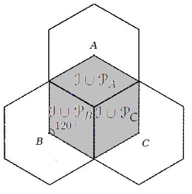
Figure 1: 3-cells system model and the frequency reuse scheme

Consider the downlink of a sectorized OFDMA cellular network composed of hexagonal cells. Each cell in the system is divided into three $120\,^{\circ}$ sectors. In this paper, we restrict ourselves to the case of three interfering sectors of three adjacent cells, say cells $A,B,C$ (see Figure 1). In the more general case of networks with more than three cells, our results hold provided that the interference generated by farther base stations can be neglected. Generally, this assumption is only valid as a first approximation. However, it allows for an essential reduction of the dimensionality of the multicell resource allocation problem. In the sequel, we assume that the considered sectors of cells $A,B,C$ have the same surface and we denote by $K^{A},K^{B},K^{C}$ their respective number of users. Let $K=K^{A}+K^{B}+K^{C}$ be the total number of users and $N$ the total number of available subcarriers. The signal received by user $k$ in cell $c$ ($c\in\{A,B,C\}$) at subcarrier $n\in\{0\ldots N-1\}$ during the $m$th OFDM block is given by

$$y_{k}(n,m)=H_{k}^{c}(n,m)s_{k}(n,m)+w_{k}(n,m)\>,$$ (1)

where $s_{k}(n,m)$ represents the data symbol destined to user $k$, and where $w_{k}(n,m)$ is a random process that encompasses both the thermal noise and the possible multicell interference. Random variable $H_{k}^{c}(n,m)$ stands for the frequency-domain channel coefficient associated with user $k$ in cell $c$ at the $n$th subcarrier and the $m$th OFDM block. The realizations of this random variable are assumed to be known only at the receiver side and unknown at the base station. Random variables $\{H_{k}^{c}(n,m)\}_{n,m}$ are Rayleigh distributed with variance $\rho_{k}=\mathbb{E}[|H_{k}^{c}(m,n)|^{2}]$ which is assumed to be constant w.r.t $n$ and $m$. This holds for example in the case of uncorrelated time-domain channel coefficients. Furthermore, for each $n\in\{0\ldots N-1\}$, random process $\{H_{k}^{c}$ $(n$, $m)\}_{m}$ is assumed to be ergodic. Finally, variance $\rho_{k}$ is assumed to be known at the transmitter side and vanishes with the distance between base station $c$ and user $k$ following a given path loss model. We assume that fractional frequency reuse is applied. According to this scheme (see Figure 1), a certain subset of subcarriers $\mathcal{I}\subset\{0\ldots N-1\}$ is reused in the three cells. If user $k$ modulates a subcarrier $n\in\mathcal{I}$, the noise $w_{k}(n,m)$ includes both thermal noise and multicell interference. The reuse factor $\alpha$ is the ratio between the number of reused subcarriers and the total number of subcarriers:

$$\alpha=\frac{\mbox{card}(\mathcal{I})}{N}\>.$$

The remaining $(1-\alpha)N$ subcarriers are shared by the three sectors in an orthogonal way, such that each base station $c$ ($c=A,B,C$) has at its disposal a subset $\mathcal{P}_{c}$ of cardinality $\frac{1-\alpha}{3}N$. If user $k$ modulates a subcarrier $n\in\mathcal{P}_{c}$, process $w_{k}(n,m)$ will contain only thermal noise with variance $\sigma^{2}$. Finally, $\mathcal{I}\cup\mathcal{P}_{A}\cup\mathcal{P}_{B}\cup\mathcal{P}_{C}=\{0,1,\ldots,N-1\}$. Denote by $\mathcal{N}_{k}$ the subset of subcarriers assigned to user $k$. We assume that $\mathcal{N}_{k}$ may contain subcarriers from both the “interference” subset $\mathcal{I}$ and the “protected” subset $\mathcal{P}_{c}$. Denote by $\gamma_{k,1}^{c}N$ (resp. $\gamma_{k,2}^{c}N$) the number of subcarriers assigned to user $k$ in $\mathcal{I}$ (resp. $\mathcal{P}_{c}$). In other words,

$$\gamma_{k,1}^{c}=\mbox{card}(\mathcal{I}\cap\mathcal{N}_{k})/N\qquad\gamma_{k,2}^{c}=\mbox{card}(\mathcal{P}_{c}\cap\mathcal{N}_{k})/N\>.$$

Parameters $\gamma_{k,1}^{c}$ and $\gamma_{k,2}^{c}$ are generally referred to as sharing factors. We assume from now on that they can take on any value in the interval $[0,1]$ (not necessarily integer multiples of $1/N$).

Remark 1.

Even when the sharing factors are not integer multiples of $1/N$, it is still possible to practically achieve the exact values of $\gamma_{k,1}^{c}$, $\gamma_{k,2}^{c}$ by simply exploiting the time dimension. Indeed, the number of subcarriers assigned to user $k$ can be chosen to vary from one OFDM symbol to another in such a way that the average number of subcarriers in subsets $\mathcal{I}$ and $\mathcal{P}_{c}$ is equal to $\gamma_{k,1}^{c}N$ and $\gamma_{k,2}^{c}N$ respectively. Thus the fact that $\gamma_{k,1}^{c}$, $\gamma_{k,2}^{c}$ are not strictly integer multiples of $1/N$ is not restrictive, provided that the system is able to grasp the benefits of the time dimension. The particular case where the number of subcarriers is restricted to be the same in each OFDM block is addressed in Section VI.

Note that by definition

$$\sum_{k=1}^{K^{c}}\gamma_{k,1}^{c}\leq\alpha\>,\qquad\sum_{k=1}^{K^{c}}\gamma_{k,2}^{c}\leq\frac{1-\alpha}{3}\>.$$

For the sake of readability and compactness of the paper, the above two inequality constraints will be written from now on as equalities i.e., we force the whole set of available subcarriers to be fully occupied by setting $\sum_{k=1}^{K^{c}}\gamma_{k,1}^{c}=\alpha$ and $\sum_{k=1}^{K^{c}}\gamma_{k,2}^{c}=\frac{1-\alpha}{3}$. Indeed, keeping the above constraints as inequalities would make the presentation of the final results as well as of the proofs very tedious.

Recall that in our model, for each user $k$ in any cell $c$, all channel coefficients $H_{k}^{c}(n,m)$ are identically distributed on all the subcarriers assigned to this user (the variance $\rho_{k}=\mathbb{E}[|H_{k}^{c}(m,n)|^{2}]$ is assumed to be constant w.r.t $n$). It is thus reasonable to assume that the base station modulates the subcarriers of each user in each one of the two subsets ($\cal I$ and $\mathcal{P}_{c}$) with the same transmit power. Define $P_{k,1}^{c}$ (resp. $P_{k,2}^{c}$) as the power transmitted on the subcarriers assigned to user $k$ in $\mathcal{I}$ (resp. in $\mathcal{P}_{c}$) i.e., $P_{k,1}^{c}=E[|s_{k}(n,m)|^{2}]$ if $n\in\mathcal{I}$, $P_{k,2}^{c}=E[|s_{k}(n,m)|^{2}]$ if $n\in\mathcal{P}_{c}$. Parameters $\{\gamma_{k,i}^{c},P_{k,i}^{c}\}_{i=1,2}$ will be designated in the sequel as the resource allocation parameters. We now describe the adopted model for the multicell interference. Consider one of the non protected subcarriers $n$ assigned to user $k$ of cell $A$ in subset $\mathcal{I}$. Denote by $\sigma_{k}^{2}$ the variance of the additive noise process $w_{k}(n,m)$. This variance is assumed to be constant w.r.t both $n$ and $m$. It depends only on the position of user $k$ and the average powers $Q_{1}^{B}=\sum_{k=1}^{K^{B}}\gamma_{k,1}^{B}P_{k,1}^{B}$ and $Q_{1}^{C}=\sum_{k=1}^{K^{C}}\gamma_{k,1}^{C}P_{k,1}^{C}$ transmitted respectively by base stations $B$ and $C$ on the subcarriers of $\cal I$. This assumption is valid for instance in OFDMA systems that utilize random subcarrier assignment [21]. According to this subcarrier assignment scheme, each user $k$ is assigned a subset $\mathcal{N}_{k}$ that is composed by randomly selecting $\textrm{card}\left(\mathcal{N}_{k}\right)$ subcarriers out of the total $N$ available subcarriers. Finally, let $\sigma^{2}$ designate the variance of the thermal noise. Putting all pieces together:

$$\mathbb{E}\left[|w_{k}(n,m)|^{2}\right]=\left\{\begin{array}[]{ll}\sigma^{2}&\mbox{if }n\in\mathcal{P}_{c}\\ \sigma_{k}^{2}=\sigma^{2}+\sum_{\tilde{c}=B,C}\mathbb{E}\left[|H_{k}^{\tilde{c}}(n,m)|^{2}\right]Q_{1}^{\tilde{c}}&\mbox{if }n\in\mathcal{I}\end{array}\right.$$ (2)

where $H_{k}^{\tilde{c}}(n,m)$ ($\tilde{c}=B,C$) represents the channel between base station $\tilde{c}$ and user $k$ in cell $c$ on subcarrier $n$ and OFDM block $m$. Of course, the average channel gain $\mathbb{E}\left[|H_{k}^{\tilde{c}}(n,m)|^{2}\right]$ depends on the position of user $k$ via the path loss model. For instance, if two users $k$ and $l$ of cell $A$ are located on the same line perpendicular to the axis $BC$ such that $k$ is closer to base station $A$, then $\sigma_{k}^{2}\leq\sigma_{l}^{2}$.

III Joint Resource Allocation Problem

Assume that each user $k$ has a rate requirement of $R_{k}$ nats/s/Hz. Consider the problem of determination of the resource allocation parameters for the three interfering sectors. These parameters must be selected such that the target rate of each user is satisfied and such that the power spent by the three base stations is minimized. Due to the ergodicity of the process $\{H_{k}^{c}(n,m)\}_{m}$ for each subcarrier $n$, the rate $R_{k}$ can be satisfied provided that it is smaller than the ergodic capacity $C_{k}$ associated with user $k$. Unfortunately, the exact expression of $C_{k}$ is difficult to obtain due to the fact that the noise-plus-interference $\{w_{k}(n,m)\}_{n,m}$ is not a Gaussian process in general. Nonetheless, if we endow the input symbols $s_{k}(n,m)$ with Gaussian distribution, the mutual information between $s_{k}(n,m)$ and the received signal $y_{k}(n,m)$ in (1) is minimal when $w_{k}(n,m)$ is Gaussian distributed. Therefore, we approximate in the sequel the multicell interference by a Gaussian process as this approximation provides a lower bound on the mutual information. Focus on cell $A$ and denote by $g_{k,1}(Q_{1}^{B},Q_{1}^{C})$, $g_{k,2}$ the channel Gain-to-Interference-plus-Noise Ratio (GINR) and Gain-to-Noise Ratio (GNR) associated with user $k$ on the subcarriers of subset $\mathcal{I}$ and $\mathcal{P}_{A}$ respectively:

$$g_{k,1}(Q_{1}^{B},Q_{1}^{C})=\frac{\rho_{k}}{\sigma_{k}^{2}}\>,\qquad g_{k,2}=\frac{\rho_{k}}{\sigma^{2}}\>.$$

The ergodic capacity $C_{k}$ associated with user $k$ in cell $A$ is equal to the sum of the ergodic capacities corresponding to both subsets $\cal I$ and ${\cal P}_{A}$. For instance, the part of the capacity corresponding to the protected subset ${\cal P}_{A}$ is equal to $\gamma_{k,2}^{A}{\mathbb{E}}\left[\log\left(1+P_{k,2}^{A}\frac{|H_{k}^{A}(n,m)|^{2}}{\sigma^{2}}\right)\right]$, where factor $\gamma_{k,2}^{A}$ traduces the fact that the capacity increases with the number of subcarriers which are modulated by user $k$. In the latter expression, the expectation is calculated w.r.t random variable $\frac{|H_{k}^{A}(m,n)|^{2}}{\sigma^{2}}$. Now, $\frac{H_{k}^{A}(m,n)|^{2}}{\sigma^{2}}$ has the same distribution as $\frac{\rho_{k}}{\sigma^{2}}Z=g_{k,2}Z$, where $Z$ follows a standard unit-variance exponential distribution. Finally, the ergodic capacity $C_{k}=C_{k}(\gamma_{k,1}^{A},\gamma_{k,2}^{A},P_{k,1}^{A},P_{k,2}^{A},Q_{1}^{B},Q_{1}^{C})$ in the whole bandwidth is equal to

$$C_{k}=\gamma_{k,1}^{A}\mathbb{E}\left[\log\left(1+g_{k,1}(Q_{1}^{B},Q_{1}^{C})P_{k,1}^{A}Z\right)\right]+\gamma_{k,2}^{A}\mathbb{E}\left[\log\left(1+g_{k,2}P_{k,2}^{A}Z\right)\right]\>.$$ (3)

Capacity $C_{k}$ is achieved if we endow the input symbols $s_{k}(n,m)$ with Gaussian distribution. This distribution is assumed from now on. Moreover, note that $C_{k}$ does not depend on the particular subcarriers $\mathcal{N}_{k}$ assigned to user $k$, but rather on the number of these subcarriers via parameters $\gamma_{k,1}^{A}$ and $\gamma_{k,2}^{A}$. Therefore, choosing some specific subcarriers rather than others has no effect on the capacity. The subcarriers assignment scheme reduces thus to the determination of the sharing factors $\gamma_{k,1}^{A}$, $\gamma_{k,2}^{A}$. Finally, the multicell resource allocation problem can be defined as follows.

Problem 1.

Minimize the power spent by the three base stations $Q=$ $\displaystyle\sum_{c=A,B,C}\sum_{k=1}^{K^{c}}(\gamma_{k,1}^{c}P_{k,1}^{c}+\gamma_{k,2}^{c}P_{k,2}^{c})$ w.r.t $\{\gamma_{k,1}^{c},\gamma_{k,2}^{c},P_{k,1}^{c},P_{k,2}^{c}\}_{\begin{subarray}{c}c=A,B,C\\ k=1\ldots K^{c}\end{subarray}}$ under the following constraints:

$$\mathbf{C1:}\> \forall k,C_{k}(\gamma_{k,1}^{c},\gamma_{k,2}^{c},P_{k,1}^{c},P_{k,2}^{c})\geq R_{k} \mathbf{C3:}\>\sum_{k=1}^{K^{c}}\gamma_{k,2}^{c}=\frac{1-\alpha}{3}$$

$$\mathbf{C2:}\> \sum_{k=1}^{K^{c}}\gamma_{k,1}^{c}=\alpha \mathbf{C4:}\>\forall k,\>\gamma_{k,i}^{c},P_{k,i}^{c}\geq 0\>(i=1,2)\>.$$

As a matter of fact, Problem 1 cannot be solved using convex optimization tools. Anyhow, even if we were able to propose a method to solve this problem (as we did in [19] in the case of 1-D networks), such a method would be very costly in term of computational complexity. It is therefore of interest to propose practical allocation algorithms that provides suboptimal solutions to Problem 1.

IV Proposed Resource Allocation Algorithm

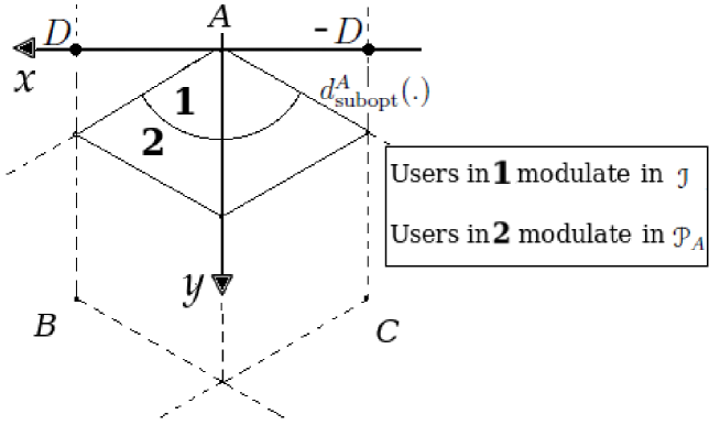
Figure 2: Fixed separating curve in cell $A$

In [20], we showed that in 1-D cellular networks, any global solution to Problem 1 has the following asymptotic property: The power allocated to users who modulate both protected and non protected subcarriers becomes negligible as the number $K$ of users increases. One can thus suggest the suboptimal (w.r.t Problem 1) resource allocation algorithm given below. For a given user $k$ in cell $c$, we denote by $(x_{k},y_{k})$ his/her position in the Cartesian coordinate system associated with this cell (see Figure 2). In our algorithm, we use a continuous function $d_{\textrm{subopt}}^{c}(.)$ on $[-D,D]$ (where $D$ stands for the radius of the cell as shown in Figure 2) to define a curve that separates the users of each cell $c$ into two subsets. The first subset $\mathcal{K}_{I}^{c}$ contains the users who are closer to the base station than this curve. These users are constrained to modulate only non protected subcarriers $\cal I$. The second subset $\mathcal{K}_{P}^{c}$ contains the rest of users who are constrained to the protected subcarriers $\mathcal{P}_{c}$:

$$\mathcal{K}_{I}^{c}=\{k\in\{1\ldots K^{c}\}\>|\>y_{k}\leq d_{\textrm{subopt}}^{c}(x_{k})\}\>,\qquad\mathcal{K}_{P}^{c}=\{k\in\{1\ldots K^{c}\}\>|\>y_{k}>d_{\textrm{subopt}}^{c}(x_{k})\}\>.$$

Note that $\{d_{\textrm{subopt}}^{c}(.)\}_{c=A,B,C}$ are fixed prior to resource allocation. Relevant selection of these curves is postponed to Subsection V-B. It merely relies on the asymptotic analysis carried out in Subsection V-A.

IV-A Resource Allocation for Interfering Users $\boldsymbol{\{{\cal K}^{c}_{I}\}_{c=A,B,C}}$

For users ${\cal K}^{c}_{I}$ in each cell $c$, resource allocation parameters in the protected subset $\mathcal{P}_{c}$ are arbitrarily set to zero i.e., $\gamma_{k,2}^{c}=P_{k,2}^{c}=0$. Recall the definition of $Q_{1}^{c}=\sum_{k\in{\cal K}_{I}^{c}}\gamma_{k,1}^{c}P_{k,1}^{c}$ as the average power transmitted by base station $c$ ($c=A,B,C$) in the interference subset $\cal I$. For each cell $c$, denote by $\bar{c}$ and $\bar{\bar{c}}$ the other two cells. For example, $\bar{A}=B$ and $\bar{\bar{A}}=C$. Define $C_{k}($ $\gamma_{k,1}^{c}$, $P_{k,1}^{c}$, $Q_{1}^{\bar{c}}$, $Q_{1}^{\bar{\bar{c}}})$ as the ergodic capacity associated with user $k$ obtained by plugging $\gamma_{k,2}^{c}=P_{k,2}^{c}=0$ into (3). Parameters $\gamma_{k,1}^{c},P_{k,1}^{c}$ for users in $\{{\cal K}_{I}^{c}\}_{c=A,B,C}$ can be obtained as the solution to the following multicell allocation problem.

Problem 2.

[Multicell problem in band $\boldsymbol{\mathcal{I}}$] Minimize the total transmit power $\displaystyle\sum_{c=A,B,C}\sum_{k\in{\cal K}_{I}^{c}}\gamma_{k,1}^{c}P_{k,1}^{c}$ w.r.t. $\{\gamma_{k,1}^{c}$, $P_{k,1}^{c}\}_{\stackrel{{\scriptstyle c=A,B,C}}{{k=1\ldots K^{c}}}}$ under the following constraints:

$$\mathbf{C1:}\>\forall c,\;\forall k\in{\cal K}_{I}^{c},R_{k}\leq C_{k}(\gamma_{k,1}^{c},P_{k,1}^{c},Q_{1}^{\bar{c}},Q_{1}^{\bar{\bar{c}}})$$

$$\mathbf{C2:}\>\forall c,\;\sum_{k\in{\cal K}_{I}^{c}}\gamma_{k,1}^{c}=\alpha\qquad\mathbf{C3:}\>\forall c,\forall k\in{\cal K}_{I}^{c},\>\gamma_{k,1}^{c},P_{k,1}^{c}\geq 0\>.$$

Remark 2.

Problem 2 may not be always feasible. Indeed, since the protected subcarriers are forbidden to users $\mathcal{K}_{I}^{c}$, the multicell interference may in some cases reach excessive levels and prevent some users from satisfying their rate requirements. Fortunately, we will see that if curves $\{d_{\textrm{subopt}}^{c}(.)\}_{c=A,B,C}$ are relevantly chosen, then the latter problem is feasible, at least for a sufficiently large number of users.

One can use an approach similar to [19, 20] to show that any global solution to the above problem satisfies the following property. There exist six positive numbers $\{\beta_{1}^{c},Q_{1}^{c}\}_{c=A,B,C}$ (where $\beta_{1}^{c}$ is the Lagrange multiplier associated with constraint $\mathbf{C2}$ of Problem 2) such that:

$$P_{k,1}^{c}=\left[g_{k,1}(Q_{1}^{\bar{c}},Q_{1}^{\bar{\bar{c}}})\right]^{-1}f^{-1}(g_{k,1}(Q_{1}^{\bar{c}},Q_{1}^{\bar{\bar{c}}})\beta_{1}^{c})$$ (4)

$$\gamma_{k,1}^{c}=\frac{R_{k}}{C\left(g_{k,1}(Q_{1}^{\bar{c}},Q_{1}^{\bar{\bar{c}}})\beta_{1}^{c}\right)}\>,$$ (5)

where $f(.)$ and $C(.)$ are increasing functions defined on ${\mathbb{R}}_{+}$ by

$$f(x)=\frac{{\mathbb{E}}\left[\log(1+xZ)\right]}{{\mathbb{E}}\left[\frac{Z}{1+xZ}\right]}-x\>,\qquad C(x)=\mathbb{E}[\log(1+f^{-1}(x)Z)]\>,$$ (6)

$f^{-1}(.)$ being the inverse on $\mathbb{R}_{+}$ of $f(.)$ w.r.t the composition of functions, and where for each $c=A,B,C$ and for a fixed value of $Q_{1}^{\bar{c}}$ and $Q_{1}^{\bar{\bar{c}}}$, $(\beta_{1}^{c},Q_{1}^{c})$ is the unique solution to the following system of equation:

$$\sum_{k\in{\cal K}_{I}^{c}}\frac{R_{k}}{C(g_{k,1}(Q_{1}^{\bar{c}},Q_{1}^{\bar{\bar{c}}})\beta_{1}^{c})}=\alpha\>,$$ (7)

$$Q_{1}^{c}=\sum_{k\in{\cal K}_{I}^{c}}R_{k}\frac{\left[g_{k,1}(Q_{1}^{\bar{c}},Q_{1}^{\bar{\bar{c}}})\right]^{-1}f^{-1}(g_{k,1}(Q_{1}^{\bar{c}},Q_{1}^{\bar{\bar{c}}})\beta_{1}^{c})}{C(g_{k,1}(Q_{1}^{\bar{c}},Q_{1}^{{\bar{\bar{c}}}})\beta_{1}^{c})}\>.$$ (8)

Note that equation (7) is equivalent to the constraint $\bf C2$: $\sum_{k}\gamma_{k,1}^{c}$ $=$ $\alpha$, while equation (8) is nothing else than the definition of the average power $Q_{1}^{c}=\sum_{k\in{\cal K}_{I}^{c}}\gamma_{k,1}^{c}P_{k,1}^{c}$ transmitted by base station $c$ in subset $\mathcal{I}$. We now prove that when Problem 2 is feasible, then the system of six equations (7)-(8) for $c=A,B,C$ admits a unique solution $\beta_{1}^{A}$, $Q_{1}^{A}$, $\beta_{1}^{B}$, $Q_{1}^{B},\beta_{1}^{C}$, $Q_{1}^{C}$ and that this solution can be obtained by a simple iterative algorithm. Focus on a given cell $c$ ($c=A,B,C$) and consider any fixed values $Q_{1}^{\bar{c}}$, $Q_{1}^{\bar{\bar{c}}}$. Denote by $I^{c}\left(Q_{1}^{\bar{c}},Q_{1}^{\bar{\bar{c}}}\right)$ the rhs of (8) i.e.,

$$I^{c}\left(Q_{1}^{\bar{c}},Q_{1}^{\bar{\bar{c}}}\right)=\sum_{k\in{\cal K}_{I}^{c}}R_{k}\frac{\left[g_{k,1}(Q_{1}^{\bar{c}},Q_{1}^{\bar{\bar{c}}})\right]^{-1}f^{-1}(g_{k,1}(Q_{1}^{\bar{c}},Q_{1}^{\bar{\bar{c}}})\beta_{1}^{c})}{C(g_{k,1}(Q_{1}^{\bar{c}},Q_{1}^{{\bar{\bar{c}}}})\beta_{1}^{c})}\>,$$

where $\beta_{1}^{c}$ is defined as the unique solution to (7). The value $I^{c}\left(Q_{1}^{\bar{c}},Q_{1}^{\bar{\bar{c}}}\right)$ can be seen as the minimum power that should be spent by base station $c$ on the interference subcarriers $\cal I$ when the interference produced by base stations ${\bar{c}}$ and $\bar{\bar{c}}$ is equal to $Q_{1}^{\bar{c}}$ and $Q_{1}^{\bar{\bar{c}}}$, respectively. Since (8) should be satisfied for $c=A$, $c=B$ and $c=C$, the following three equations hold

$$Q_{1}^{A}=I^{A}(Q_{1}^{B},Q_{1}^{C}),\quad Q_{1}^{B}=I^{B}(Q_{1}^{A},Q_{1}^{C}),\quad Q_{1}^{C}=I^{C}(Q_{1}^{A},Q_{1}^{B})\>.$$

The triple $(Q_{1}^{A},Q_{1}^{B},Q_{1}^{C})$ is therefore clearly a fixed point of the vector-valued function ${\bf I}(Q_{1}^{A},Q_{1}^{B},Q_{1}^{C})$ $=$ $\left(I^{A}(Q_{1}^{B},Q_{1}^{C}),I^{B}(Q_{1}^{A},Q_{1}^{C}),I^{C}(Q_{1}^{A},Q_{1}^{B})\right)$:

$$(Q_{1}^{A},Q_{1}^{B},Q_{1}^{C})={\bf I}(Q_{1}^{A},Q_{1}^{B},Q_{1}^{C})\>.$$ (9)

As a matter of fact, it can be shown that such a fixed point of ${\bf I}$ is unique. This claim can be proved using the following lemma.

Lemma 1.

Function ${\bf I}$ is such that the following properties hold.

1. Positivity: ${\mathbf{I}}(Q^{A},Q^{B},Q^{C})>0$.

2. Monotonicity: If $Q^{A}\geq{Q^{A}}^{\prime},Q^{B}\geq{Q^{B}}^{\prime},Q^{C}\geq{Q^{C}}^{\prime}$, then ${\mathbf{I}}(Q^{A},Q^{B},Q^{C})\geq{\mathbf{I}}({Q^{A}}^{\prime},{Q^{B}}^{\prime},{Q^{C}}^{\prime})$.

3. Scalability: for all $t>1$, $t{\mathbf{I}}(Q^{A},Q^{B},Q^{C})>{\mathbf{I}}(tQ^{A},tQ^{B},tQ^{C})$.

The proof of Lemma 1 uses arguments which are very similar to the proof of Theorem 1 in [23]. Function ${\mathbf{I}}$ is then a standard interference function, using the terminology of [24]. Therefore, as stated in [24], such a function ${\bf I}$ admits at most one fixed point. On the other hand, the existence of a fixed point is ensured by the feasibility of Problem 2 and by the fact that (9) holds for any global solution. In other words, if Problem 2 is feasible, then function ${\bf I}$ does admit a fixed point and this fixed point is unique. In the latter case, the results of [24] state furthermore that a simple fixed point algorithm (such as Algorithm 1 given below) applied to function $\mathbf{I}$ converges necessarily to its unique fixed point.

Remark 3.

Note that in Algorithm 1, the only information needed by each base station $c$ ($c=A,B,C$) about the other two cells $\bar{c}$, $\bar{\bar{c}}$ is the current value of the powers $Q_{1}^{\bar{c}}$, $Q_{1}^{\bar{{\bar{c}}}}$ transmitted in the interference band $\cal I$. This value can i) either be measured by base station $c$ at each iteration of Algorithm 1, or ii) it can be communicated to it by base stations $\bar{c}$ and $\bar{\bar{c}}$ over a dedicated link. In the first case, no message passing is required, and in the second case only few information is exchanged between the base stations. Algorithm 1 can thus be implemented in a distributed fashion.

Of course, the feasibility of Problem 2 depends on the choice of the separating curves $\{d_{\textrm{subopt}}^{c}(.)\}_{c=A,B,C}$. Section V addresses the relevant selection of these curves such that Algorithm 1 converges for a sufficiently large number of users.

IV-B Resource Allocation for Protected Users $\boldsymbol{\{{\cal K}^{c}_{P}\}_{c=A,B,C}}$

Since users ${\cal K}^{c}_{P}$ in each cell $c$ are constrained to modulate only the subcarriers of subset $\mathcal{P}_{c}$, they are not subject to multicell interference. Resource allocation for such users can thus be done independently in each cell by solving a simple single cell optimization problem which is a special case of Problem 2. Focus for example on cell $A$. One can show [19] that the resource allocation problem for users of this cell is convex in variables $\{\gamma_{k,2}^{A},w_{k,2}^{A}\}_{k\in{\cal K}^{A}_{P}}$, where $w_{k,2}^{A}=\gamma_{k,2}^{A}P_{k,2}^{A}$. Its solution can be obtained by solving the associated KKT conditions and is given by:

$$P_{k,2}^{A}=g_{k,2}^{-1}f^{-1}(g_{k,2}\beta_{2}^{A})$$ (10)

$$\gamma_{k,2}^{A}=\frac{R_{k}}{C\left(g_{k,2}\beta_{2}^{A}\right)}\>.$$ (11)

Parameter $\beta_{2}^{A}$ is obtained by writing that constraint $\sum_{k}\gamma_{k,2}^{A}=\frac{1-\alpha}{3}$ holds as the unique solution to:

$$\sum_{k\in{\cal K}^{A}_{P}}\frac{R_{k}}{C(g_{k,2}\beta_{2}^{A})}=\frac{1-\alpha}{3}\>.$$ (12)

Resource allocation parameters for users of cells $B$ and $C$ can be similarly obtained. The following procedure performs the above resource allocation for protected users.

IV-C Summary: Distributed Resource Allocation Algorithm

The proposed distributed resource allocation scheme is finally summarized by Algorithm 3.

IV-D Complexity Analysis

By referring to Algorithm 2, it is straightforward to verify that resource allocation for protected users can be reduced to the determination in each cell $c$ of the value of $\beta_{2}^{c}$, which is the unique solution to the equation $\sum_{k\in{\cal K}^{c}_{P}}\frac{R_{k}}{C(g_{k,2}\beta_{2}^{c})}=\frac{1-\alpha}{3}$. Since function $x\mapsto 1/C(x)$ is convex, the latter solution can be numerically obtained by any of the classical zero-finding algorithms of the convex optimization literature such as the gradient method [25]. Denote by $N_{\textrm{grad}}$ the number of iterations required till the convergence of such a method. Each one of these iterations requires a computational complexity proportional to the number of terms in the lhs of the equation. The overall computational complexity of finding $\beta_{2}^{c}$ is therefore of order $O(N_{\textrm{grad}}K)$. In the same way, one can show that each iteration of Algorithm 1 can be performed with a complexity of order $O(N_{\textrm{grad}}K)$. Let $N_{\textrm{iter}}$ designate the number of iterations of Algorithm 1 needed till convergence (within a certain accuracy). The overall computational complexity of Algorithm 1, and hence of Algorithm 3 as well, is thus of the order of $O(N_{\textrm{iter}}N_{\textrm{grad}}K)$. Our simulations showed that Algorithm 1 converges relatively quickly in most of the cases. Indeed, no more than $N_{\textrm{iter}}=15$ iterations were needed to reach convergence within a very reasonable accuracy in most of the practical situations.

V Determination of Curves $\boldsymbol{\{{d}_{\textrm{{subopt}}}^{{c}}(.)\}}$ and Asymptotic Optimality of Algorithm 3

The aim of this section is to relevantly select the separating curves $d_{\textrm{subopt}}^{A}(.)$, $d_{\textrm{subopt}}^{B}(.)$ and $d_{\textrm{subopt}}^{C}(.)$. For that sake, we consider the case where the number $K$ of users tends to infinity in a sense that will be clear later on, and we prove Theorem 1 (see Subsection V-C) which states the following. There exist curves $\{d_{\textrm{subopt}}^{c}(.)\}_{c=A,B,C}$ such that the transmit power of Algorithm 3 converges as $K\to\infty$ to the limit total power of an optimal solution to the joint allocation problem (Problem 1). Otherwise stated, Algorithm 3 is asymptotically optimal if the separating curves are well chosen. In order to prove this result, we first characterize the form and the total transmit power $Q_{T}^{(K)}$ of an optimal solution to Problem 1 in the special case where users of each cell are aligned on parallel equispaced lines. Indeed, we prove that the latter solution has the following “binary” property: In each cell $c$, there exists a curve $d_{\theta^{c,(K)}}$ that separates users modulating uniquely protected or non protected subcarriers. Here, $\theta^{c,(K)}$ is a vector of parameters that will be specified later on and which depends on the system setting (including the number $K$ of users). We show that as the number $K$ of users tends to infinity, $d_{\theta^{c,(K)}}$ converges, at least for certain subsequences $(K)$, to a curve $d_{\theta^{c}}$ that can be characterized by solving a certain system of equations. The same system allows to compute the limit $Q_{T}=\lim_{K\to\infty}Q_{T}^{(K)}$. Next, we consider the case of an arbitrary geographical distribution where users are not necessarily aligned on parallel lines. Eventhough the aforementioned binary property no longer holds in this general case, we show that the transmit power of an optimal solution to Problem 1 converges to the same limit $Q_{T}$ as in the case of aligned users. This result will suggest to relevantly select the separating curves $d_{\textrm{subopt}}^{c}(.)$ of the suboptimal allocation algorithm to be equal to the asymptotic optimal curves $d_{\theta^{c}}(.)$. Thanks to the latter curve selection, we prove that the proposed allocation algorithm becomes asymptotically optimal.

V-A Asymptotic Optimal Allocation

The characterization of the asymptotic behaviour of an optimal solution to the joint resource allocation problem is performed by the following three steps.

V-A1 Step 1: Single Cell Resource Allocation

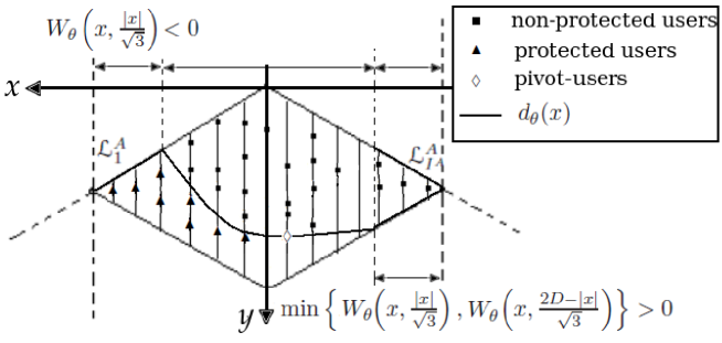
Figure 3: Definition of subsets $\{\mathcal{L}_{i}^{A}\}_{i=1\ldots I^{A}}$ and of the curve $d_{\theta}(.)$

We first consider a particular case where users of each cell are aligned on equispaced parallel lines. Focus for example on cell $A$ and define $I^{A}$ parallel equispaced lines ($I^{A}<K^{A}$) which pass through cell $A$ and which are perpendicular to the axis $BC$ as illustrated in Figure 3. Next, assign each one of these lines an index $i\in\{1\ldots I^{A}\}$. In the sequel, we denote by $\mathcal{L}_{i}^{A}\subset\{1\ldots K^{A}\}$ the subset composed of the users of cell $A$ located on the line whose index is $i$. Assume that the resource allocation parameters of users of cells $B$ and $C$ are fixed and recall the definition of $C_{k}$ given by (3) as the ergodic capacity of user $k$. The optimal resource allocation problem for cell $A$ consists in characterizing $\{\gamma_{k,1}^{A}$, $\gamma_{k,2}^{A}$, $P_{k,1}^{A}$, $P_{k,2}^{A}\}_{k=1\ldots K^{A}}$ allowing to satisfy the rate requirements of all users $k\in\{1,\ldots,K^{A}\}$. The determination of these parameters should be done such that the power $Q^{A}=\sum_{k=1}^{K^{A}}\gamma_{k,1}^{A}P_{k,1}^{A}+\gamma_{k,2}^{A}P_{k,2}^{A}$ to be spent is minimum:

Problem 3.

Minimize $Q^{A}=\sum_{k=1}^{K^{A}}\gamma_{k,1}^{A}P_{k,1}^{A}+\gamma_{k,2}^{A}P_{k,2}^{A}$ with respect to $\{\gamma_{k,1}^{A}$, $\gamma_{k,2}^{A}$, $P_{k,1}^{A}$, $P_{k,2}^{A}\}_{k=1\ldots K^{A}}$ under the following constraints:

$$\mathbf{C1:}\> \forall k,R_{k}\leq C_{k} \mathbf{C4:}\>\gamma_{k,1}^{A}\geq 0,\gamma_{k,2}^{A}\geq 0$$

$$\mathbf{C2:}\> \sum_{k=1}^{K^{A}}\gamma_{k,1}^{A}=\alpha \mathbf{C5:}\>P_{k,1}^{A}\geq 0,P_{k,2}^{A}\geq 0.$$

$$\mathbf{C3:}\> \sum_{k=1}^{K^{A}}\gamma_{k,2}^{A}=\frac{1-\alpha}{3} {\bf C6:}\>\sum_{k=1}^{K^{A}}\gamma_{k,1}^{A}P_{k,1}^{A}\leq{\cal Q}\>.$$

Here, constraint $\bf C6$ is a “low nuisance constraint” which is introduced to limit the interference produced by Base Station $A$. In other words, the power $Q_{1}^{A}=\sum_{k}\gamma_{k,1}^{A}P_{k,1}^{A}$ which is transmitted by base station $A$ on the subcarriers of subset $\cal I$ should not exceed a certain nuisance level $\cal Q$. The introduction of $\bf C6$ is a technical tool revealed to be useful in solving the multicell allocation problem later on. On one hand, note that Problem 3 is feasible for any $\alpha>0$ and ${\cal Q}\geq 0$ since it has at least the following trivial solution. The solution consists in assigning zero power $P_{k,1}^{A}=0$ on the subcarriers of subset $\cal I$ (so that constraint $\bf C6$ will be satisfied), and in performing resource allocation only using the subcarriers of subset $\mathcal{P}_{A}$. On the other hand, Problem 3 can be made convex after a slight change of variables, as a matter of fact. Therefore, any global solution to this problem is characterized by the KKT conditions. The simplification of these conditions is not presented in this paper due to lack of space. However, it can be done in a very similar way as in the case of 1-D cellular networks addressed in our previous work [19] leading to the following result. Resource allocation parameters of any of the subsets $\mathcal{L}_{i}^{A}$ of users located on lines $i=1\ldots I^{A}$ have a “binary” separation property as the users of a 1-D cell. This property is summarized below. Define the following decreasing function for each $x\in\mathbb{R}_{+}$:

$$F(x)={\mathbb{E}}\left[\frac{Z}{1+f^{-1}(x)Z}\right]\>,$$ (13)

and let $\beta_{1}$, $\beta_{2}$ and $\xi$ designate the Lagrange multipliers associated with constraints $\bf C2$, $\bf C3$ and $\bf C6$ respectively. There exists a “pivot-position” on each line $i$ such that users $k\in\mathcal{L}_{i}^{A}$ who are farther than this position are uniquely assigned subcarriers from the protected subset $\mathcal{P}_{A}$ (by setting $\gamma_{k,1}^{A}=0$). Moreover, such “protected users” satisfy:

$$\frac{g_{k,1}\left(Q_{1}^{B},Q_{1}^{C}\right)}{1+\xi}F\left(\frac{g_{k,1}\left(Q_{1}^{B},Q_{1}^{C}\right)}{1+\xi}\beta_{1}\right)<g_{k,2}F(g_{k,2}\beta_{2})\>.$$ (14)

On the other hand, users $k\in\mathcal{L}_{i}^{A}$ who are closer to the base station than the pivot-position are uniquely assigned interference subcarriers from subset $\mathcal{I}$ (by setting $\gamma_{k,2}^{A}=0$). Such “non protected users” satisfy:

$$\frac{g_{k,1}\left(Q_{1}^{B},Q_{1}^{C}\right)}{1+\xi}F\left(\frac{g_{k,1}\left(Q_{1}^{B},Q_{1}^{C}\right)}{1+\xi}\beta_{1}\right)>g_{k,2}F(g_{k,2}\beta_{2})\>.$$ (15)

The proof of the above separation property uses Conjecture 1 in [19] which can be easily validated numerically. Inequalities (14) and (15) suggest the definition of a curve that geographically separates protected from non protected users of cell $A$. This can be done as follows. We write the variance $\rho_{k}$ of the channel gain of user $k$ as $\rho_{k}=\rho(x_{k},y_{k})$ where $\rho(x,y)$ models the path loss. Function $\rho(x,y)$ is assumed to have the form $\rho(x,y)=\eta(\sqrt{x^{2}+y^{2}})^{-s}$ where $\sqrt{x^{2}+y^{2}}$ is the distance separating $(x,y)$ from the base station, $\eta$ is a certain gain and $s$ is the path-loss coefficient. We also denote by $g_{2}(x,y)=\frac{\rho(x,y)}{\sigma^{2}}$ the GNR on the protected subcarriers associated with a user at position $(x,y)$. Note that for any user $k$, $g_{2}(x_{k},y_{k})=g_{k,2}$. In the same way, $g_{1}(x,y,{\cal Q}^{\prime},{\cal Q}^{\prime\prime})$ denotes the GINR at position $(x,y)$ if the interfering base stations are transmitting with power ${\cal Q}^{\prime}$ and ${\cal Q}^{\prime\prime}$ on the interference subcarriers $\cal I$. Using the above notation, we have $g_{1}\left(x_{k},y_{k},Q_{1}^{B},Q_{1}^{C}\right)=g_{k,1}\left(Q_{1}^{B},Q_{1}^{C}\right)$ for each user $k$ in cell $A$. Note that for any $(x,y)$, $g_{2}(x,y)=g_{1}(x,y,0,0)$. Finally, for each $\theta=(\beta_{1},\beta_{2},\mathcal{Q}^{\prime},\mathcal{Q}^{\prime\prime},\xi)\in\mathbb{R}_{+}^{5}$, we define

$$W_{\theta}(x,y)=\frac{g_{1}(x,y,\mathcal{Q}^{\prime},\mathcal{Q}^{\prime\prime})}{1+\xi}F\left(\frac{g_{1}(x,y,\mathcal{Q}^{\prime},\mathcal{Q}^{\prime\prime})}{1+\xi}\beta_{1}\right)-g_{2}(x,y)F(g_{2}(x,y)\beta_{2})\>.$$ (16)

Due to (14), we have $W_{\theta}(x_{k},y_{k})<0$ for each protected user $k$ i.e., for users farther from the base station than the pivot-position. Inversely, $W_{\theta}(x_{k},y_{k})>0$ for each non protected user $k$ i.e., for users closer to the base station than the pivot-position. Therefore, function $d_{\theta}(x)$ given below defines the curve that we are seeking and which geographically separates protected from non protected users of cell $A$:

$$\begin{multlined}d_{\theta}(x)=\left\{\begin{array}[]{ll}\frac{|x|}{\sqrt{3}}&\textrm{if }W_{\theta}\left(x,\frac{|x|}{\sqrt{3}}\right)<0\\ \frac{2D-|x|}{\sqrt{3}}&\textrm{if }\min\left\{W_{\theta}\left(x,\frac{|x|}{\sqrt{3}}\right),W_{\theta}\left(x,\frac{2D-|x|}{\sqrt{3}}\right)\right\}>0\\ \textrm{the unique zero of }y\mapsto W_{\theta}(x,y)&\textrm{otherwise}\>.\end{array}\right.\end{multlined}d_{\theta}(x)=\left\{\begin{array}[]{ll}\frac{|x|}{\sqrt{3}}&\textrm{if }W_{\theta}\left(x,\frac{|x|}{\sqrt{3}}\right)<0\\ \frac{2D-|x|}{\sqrt{3}}&\textrm{if }\min\left\{W_{\theta}\left(x,\frac{|x|}{\sqrt{3}}\right),W_{\theta}\left(x,\frac{2D-|x|}{\sqrt{3}}\right)\right\}>0\\ \textrm{the unique zero of }y\mapsto W_{\theta}(x,y)&\textrm{otherwise}\>.\end{array}\right.$$ (17)

Note in particular that the first two conditions of (17) hold in the case where the pivot-position at line $x$ is located at the upper sector border $y=|x|/\sqrt{3}$ or the lower sector border $y=\left(2D-|x|\right)/\sqrt{3}$. When these two conditions are not satisfied, the existence of the zero of the continuous function $y\mapsto W_{\theta}(x,y)$ is straightforward due to the intermediate value theorem. The uniqueness of this zero can be proved by arguments already developed in the proof of Lemma 1 in [19]. Finally, we obtain the following lemma.

Lemma 2.

Assume that the users of cell $A$ are aligned on $I^{A}$ parallel equispaced lines (as in Figure 3) and that the power transmitted by base stations $B$ and $C$ on the non protected subcarriers $\cal I$ is set to $Q_{1}^{B}$ and $Q_{1}^{C}$ respectively. The global solution $\{\gamma_{k,1}^{A},\gamma_{k,2}^{A},P_{k,1}^{A},P_{k,2}^{A}\}_{k=1\ldots K^{A}}$ to Problem 3 is unique and is as follows. There exist three unique nonnegative numbers $\beta_{1}$, $\beta_{2}$, $\xi$ such that:

1. For each $k\in{{\cal L}_{i}^{A}}$ such that $y_{k}<d_{\theta}(x_{k})$,

   $$\begin{array}[h]{l|l}\displaystyle P_{k,1}^{A}=\left[g_{k,1}\left(Q_{1}^{B},Q_{1}^{C}\right)\right]^{-1}f^{-1}\left(\frac{g_{k,1}\left(Q_{1}^{B},Q_{1}^{C}\right)}{1+\xi}\beta_{1}\right)&P_{k,2}^{A}=0\\ \displaystyle\gamma_{k,1}^{A}=\frac{R_{k}}{C\left(\frac{g_{k,1}\left(Q_{1}^{B},Q_{1}^{C}\right)}{1+\xi}\beta_{1}\right)}&\gamma_{k,2}^{A}=0\end{array}$$ (18)

2. For each $k\in{{\cal L}_{i}^{A}}$ such that $y_{k}>d_{\theta}(x_{k})$,

   $$\begin{array}[h]{l|l}P_{k,1}^{A}=0&\displaystyle P_{k,2}^{A}=g_{k,2}^{-1}f^{-1}(g_{k,2}\beta_{2})\\ \gamma_{k,1}^{A}=0&\displaystyle\gamma_{k,2}^{A}=\frac{R_{k}}{C\left(g_{k,2}\beta_{2}\right)}\end{array}$$ (19)

where $\beta_{1}$, $\beta_{2}$ and $\xi$ are the Lagrange multipliers associated with constraints $\bf C2$, $\bf C3$ and $\bf C6$ respectively, and where $\theta=\left(\beta_{1},\beta_{2},Q_{1}^{B},Q_{1}^{C},\xi\right)$. Here, $d_{\theta}(.)$ is the function defined by (17).

The uniqueness of the above global solution can be proved using arguments similar to those of the proof of Proposition 1 in [19]. Note that due to the above lemma, there is at most one user in each subset $\mathcal{L}_{i}^{A}$ who is likely to modulate both protected and non protected subcarriers. If such a “pivot-user” exists, then it is necessarily located on the curve $d_{\theta}(.)$. Therefore, there are at most $I^{A}$ pivot-users in cell $A$.

V-A2 Step 2: From Single Cell to Multicell Resource Allocation

We now consider the problem of joint resource allocation (Problem 1) while still assuming that users of each cell are aligned on equispaced parallel lines. Recall the definition of $\mathcal{L}_{i}^{c}$ as the subset of users of cell $c$ located on line $i$ ($i=1\ldots I^{c}$). The following lemma implies that any optimal solution to Problem 1 has in each cell the same form as the solution to the single cell problem given by Lemma 2.

Lemma 3.

Assume that the positions of users of each cell $c\in\{A,B,C\}$ are aligned on $I^{c}$ parallel equispaced lines. Any global solution $\{\gamma_{k,1}^{c},P_{k,1}^{c},\gamma_{k,2}^{c},P_{k,2}^{c}\}_{\stackrel{{\scriptstyle c=A,B,C}}{{k=1\ldots K^{c}}}}$ to Problem 1 satisfies the following. Let $Q_{1}^{c}=\sum_{k=1}^{K^{c}}\gamma_{k,1}^{c}P_{k,1}^{c}$ designate the power transmitted by base station $c$ on the reused subcarriers $\cal I$. There exist nine positive numbers $\{\beta_{1}^{c}$, $\beta_{2}^{c}$, $\xi^{c}\}_{c=A,B,C}$ such that (18), (19) hold in each cell.

The proof of Lemma 3 is provided in Appendix A. For each cell $c\in\{A,B,C\}$, denote by $\bar{c}$ and $\bar{\bar{c}}$ the other two cells and recall the definition of function $d_{\theta}(x)$ given by (17) for any $x\in[-D,D]$ and $\theta\in\mathbb{R}_{+}^{5}$. Lemma 3 states that when an optimal solution to Problem 1 is applied, then there exists in each cell $c=A,B,C$ a curve $d_{\theta^{c}}(.)$, where $\theta^{c}=(\beta_{1}^{c},\beta_{2}^{c},Q_{1}^{\bar{c}},Q_{1}^{\bar{\bar{c}}},\xi^{c})$, that separates protected users from non protected users.

V-A3 Step 3: Asymptotic Performance of the Optimal Resource Allocation

Denote by $\theta^{c,(K)}=\big{(}\beta_{1}^{c,(K)}$, $\beta_{2}^{c,(K)}$, $Q_{1}^{\bar{c},(K)}$, $Q_{1}^{\bar{\bar{c}},(K)}$, $\xi^{c,(K)}\Big{)}$ for $c=A,B,C$ any set of parameters chosen such that Lemma 3 holds. Superscript $(K)$ is used in order to stress the dependency of the above parameters on the number of users $K$. We now characterize the behaviour of $\theta^{c,(K)}$ as the number $K$ of users tends to infinity. Once the behaviour of $\theta^{c,(K)}$ determined, the asymptotic behaviour of both the separating curves $d_{\theta^{c,(K)}}(.)$ and the total transmit power of the optimal solution to Problem 1 can be fully characterized. Assume that the total number $K$ of users tends to infinity in such a way that $K^{c}/K\to 1/3$ i.e., the number of users in each cell is asymptotically equivalent. Denote by $B$ the total bandwidth of the system. Define $r_{k}$ as the target rate of user $k$ in nats/s i.e., $r_{k}=BR_{k}$ where $R_{k}$ is the data rate requirement of user $k$ in nats/s/Hz. Since the sum $\sum_{k}r_{k}$ of rate requirements tends to infinity, we let the bandwidth $B$ grow to infinity and we assume that $K/B\to t$ where $t$ is a positive real number. We use in the sequel the notation $I^{c,(K)}$ to designate the number of parallel equispaced lines in cell $c$. We also assume that $I^{c,(K)}$ is such that

$$I^{c,(K)}\xrightarrow[K\to\infty]{}\infty\>, \frac{I^{c,(K)}}{K}\xrightarrow[K\to\infty]{}0\>.$$

In order to simplify the proof of the results, we assume without restriction that the rate requirement $r_{k}$ for each user $k$ is upper-bounded by a certain constant $r_{\max}$ where $r_{\max}$ can be chosen as large as needed. We also assume that for each user $k$, $y_{k}\geq\epsilon$ where $\epsilon>0$ can be chosen as small as needed.

As a matter of fact, sequences $\beta_{1}^{c,(K)}$, $\beta_{2}^{c,(K)}$, $Q_{1}^{c,(K)}$, $Q_{2}^{c,(K)}$, $\xi^{c,(K)}$ are upper-bounded (refer to Appendix E in [22] for the proof). One can thus extract convergent subsequences from the above sequences. With a slight abuse of notation, $\theta^{c,(K)}=\Big{(}\beta_{1}^{c,(K)}$, $\beta_{2}^{c,(K)}$, $Q_{1}^{\bar{c},(K)}$, $Q_{1}^{\bar{\bar{c}},(K)}$, $\xi^{c,(K)}\Big{)}$ will designate from now on these convergent subsequences and their respective limits will be denoted by $\theta^{c}=(\beta_{1}^{c}$, $\beta_{2}^{c}$, $Q_{1}^{\bar{c}}$, $Q_{1}^{\bar{\bar{c}}}$, $\xi^{c})$. We now provide a system of equation satisfied by the accumulation points $\theta^{c}=(\beta_{1}^{c}$, $\beta_{2}^{c}$ $Q_{1}^{\bar{c}}$, $Q_{1}^{\bar{\bar{c}}}$, $\xi^{c})$. Due to Lemma 3, the power $Q_{1}^{c,(K)}=\sum_{k=1}^{K^{c}}\gamma_{k,1}^{c}P_{k,1}^{c}$ transmitted by base station $c$ on the non protected subcarriers $\cal I$ can be written as

$$Q_{1}^{c,(K)}=\sum_{\stackrel{{\scriptstyle k\in\{1\ldots K^{c}\}}}{{y_{k}<d_{\theta^{c,(K)}}(x_{k})}}}R_{k}{\cal F}\left(x_{k},y_{k},\beta_{1}^{c,(K)},Q_{1}^{\bar{c},(K)},Q_{1}^{\bar{\bar{c}},(K)},\xi^{c,(K)}\right)+\sum_{\stackrel{{\scriptstyle k\in\{1\ldots K^{c}\}}}{{y_{k}=d_{\theta^{c,(K)}}(x_{k})}}}\gamma_{k,1}^{c}P_{k,1}^{c}\>,$$ (20)

where function $\cal F$ is defined as

$${\cal F}(x,y,\beta,{\cal Q}^{\prime},{\cal Q}^{\prime\prime},\xi)=\frac{f^{-1}\left(\frac{g_{1}(x,y,{\cal Q}^{\prime},{\cal Q}^{\prime\prime})}{1+\xi}\beta\right)}{g_{1}(x,y,{\cal Q}^{\prime\prime},{\cal Q}^{\prime\prime})C\left(\frac{g_{1}(x,y,{\cal Q}^{\prime},{\cal Q}^{\prime\prime})}{1+\xi}\beta\right)}$$ (21)

for each $\left(x,y,\beta,{\cal Q}^{\prime},{\cal Q}^{\prime\prime},\xi\right)$ $\in[-D,-D]\times[\epsilon,D]\times\mathbb{R}_{+}^{4}$. While the first term in (20) represents the power allocated to all the users of cell $c$ that are uniquely assigned non protected subcarrier from subset $\mathcal{I}$, the second term in the same equation represents the power transmitted to the (at most) $I^{c,(K)}$ pivot-users in the same subset. Since we assume that $I^{c,(K)}/K\to 0$, one can show [22] that the latter term is negligible with respect to the first term and that it tends to zero as $K\to\infty$. Thus, it will be denoted in the sequel by $o_{K}(1)$, where $o_{K}(1)$ stands for any term that converges to zero as $K$ tends to infinity. Define for each cell $c=A,B,C$ the following measure $\nu^{c,(K)}$ on the Borel sets of $\mathbb{R}_{+}\times\mathbb{R}\times\mathbb{R}_{+}$ as

$$\nu^{c,(K)}(I,J,L)=\frac{1}{K^{c}}\sum_{k=1}^{K^{c}}\delta_{(r_{k},x_{k},y_{k})}(I,J,L)\>,$$

where $I,J,L$ are intervals of $\mathbb{R}_{+}$, $\mathbb{R}$ and $\mathbb{R}_{+}$ respectively and where $\delta_{(r_{k},x_{k},y_{k})}$ is the Dirac measure at point $(r_{k},x_{k},y_{k})$ i.e., $\delta_{(r_{k},x_{k},y_{k})}(I,J,L)=1$ if $r_{k}\in I$, $x_{k}\in J$, $y_{k}\in L$ and $\delta_{(r_{k},x_{k},y_{k})}(I,J,L)=0$ otherwise. Note that $\nu^{c,(K)}(I,J,L)$ can be interpreted as the number of users of cell $c$ whose rate requirement in nats/s is inside $I$, whose x-coordinate is inside $J$ and whose y-coordinate is inside $L$, normalized by $K^{c}$. In other words, measure $\nu^{c,(K)}$ characterizes both the geographical distribution of users in cell $c$ and their attribution to the different rate requirements. Replacing $R_{k}$ (in nats/s/Hz) by $\frac{r_{k}\mbox{ (nats/s) }}{B}$ in (20), we obtain

$$\begin{multlined}Q_{1}^{c,(K)}=\frac{K^{c}}{B}\int_{0}^{r_{\max}}\int_{-D}^{D}\int_{\max\{|x|/\sqrt{3},\epsilon\}}^{d_{\theta^{c,(K)}}(x)}r{\cal F}\left(x,y,\beta_{1}^{c,(K)},Q_{1}^{\bar{c},(K)},Q_{1}^{\bar{\bar{c}},(K)},\xi^{c,(K)}\right)d\nu^{c,(K)}(r,x,y)+o_{K}(1)\>,\end{multlined}Q_{1}^{c,(K)}=\frac{K^{c}}{B}\int_{0}^{r_{\max}}\int_{-D}^{D}\int_{\max\{|x|/\sqrt{3},\epsilon\}}^{d_{\theta^{c,(K)}}(x)}r{\cal F}\left(x,y,\beta_{1}^{c,(K)},Q_{1}^{\bar{c},(K)},Q_{1}^{\bar{\bar{c}},(K)},\xi^{c,(K)}\right)d\nu^{c,(K)}(r,x,y)+o_{K}(1)\>,$$ (22)

In the sequel, we assume that the following holds.

Assumption 1.

As $K$ tends to infinity, measure $\nu^{c,(K)}$ converges weakly to a measure $\nu^{c}$. Moreover, $\nu^{c}$ is the measure product of a limit rate distribution $\zeta^{c}$ times a limit location distribution $\lambda^{c}$. Finally, $\lambda^{c}$ is absolutely continuous with respect to the Lebesgue measure on $\mathbb{R}^{2}$.

Note that given the definition of $\zeta^{c}$, the value $\bar{R}^{c}$ defined as

$$\bar{R}^{c}=\frac{t}{3}\int_{0}^{r_{\max}}r\>d\zeta^{c}(r)$$ (23)

represents the total average rate requirement per channel use in cell $c$. Here, recall that $t$ is the limit of $K/B$ as $K\to\infty$. It is intuitive that $Q_{1}^{c,(K)}$ as given by (22) converges in this case to a constant $Q_{1}^{c}$ defined by

$$Q_{1}^{c}={\bar{R}}^{c}\int_{x=-D}^{D}\int_{y=\max\{|x|/\sqrt{3},\epsilon\}}^{d_{\theta^{c}}(x)}{\cal F}\left(x,y,\beta_{1}^{c},Q_{1}^{\bar{c}},Q_{1}^{\bar{\bar{c}}},\xi^{c}\right)\>d\lambda^{c}(x,y)\>.$$ (24)

Using the same approach as above and recalling that $g_{2}(x,y)=g_{1}(x,y,0,0)$, one can show that the power $Q_{2}^{c,(K)}$ transmitted by base station $c$ on the protected subcarriers $\mathcal{P}_{c}$ converges as $K\to\infty$ to

$$Q_{2}^{c}={\bar{R}}^{c}\int_{x=-D}^{D}\int_{y=d_{\theta^{c}}(x)}^{\frac{2D-|x|}{\sqrt{3}}}{\cal F}\left(x,y,\beta_{2}^{c},0,0,0\right)\>d\lambda^{c}(x,y)\>.$$ (25)

Now recall the expression of $\gamma_{k,1}^{c}$ given by Lemma 3 for all users $k$ satisfying $y_{k}<d_{\theta^{c,(K)}}(x_{k})$. Plugging the latter expression into constraint $\textrm{\bf C2:}\sum_{k=1}^{K^{c}}\gamma_{k,1}^{c}=\alpha$ of Problem 1, we obtain

$$\frac{1}{B}\sum_{\stackrel{{\scriptstyle k\in\{1\ldots K^{c}\}}}{{y_{k}<d_{\theta^{c,(K)}}(x_{k})}}}r_{k}{\cal G}\left(x_{k},y_{k},\beta_{1}^{c,(K)},Q_{1}^{\bar{c},(K)},Q_{1}^{\bar{\bar{c}},(K)},\xi^{c,(K)}\right)+\sum_{\stackrel{{\scriptstyle k\in\{1\ldots K^{c}\}}}{{y_{k}=d_{\theta^{c,(K)}}(x_{k})}}}\gamma_{k,1}^{c}=\alpha\>,$$ (26)

where we defined

$${\cal G}(x,y,\beta,{\cal Q}^{\prime},{\cal Q}^{\prime\prime},\xi)=\frac{1}{C\left(\frac{g_{1}(x,y,{\cal Q}^{\prime},{\cal Q}^{\prime\prime})}{1+\xi}\beta\right)}$$ (27)

for each positive $x$, $y$, $\beta$, ${\cal Q}^{\prime}$, ${\cal Q}^{\prime\prime}$ and $\xi$. It is thus quite intuitive that equation (26) leads as $K\to\infty$ to

$${\bar{R}}^{c}\int_{-D}^{D}\int_{y=\max\{|x|/\sqrt{3},\epsilon\}}^{d_{\theta^{c}}(x)}{\cal G}(x,y,\beta_{1}^{c},Q_{1}^{\bar{c}},Q_{1}^{\bar{\bar{c}}},\xi^{c})\>d\lambda^{c}(x,y)=\alpha\>.$$ (28)

Similarly, we can show that constraint $\textrm{\bf C3:}\sum_{k=1}^{K^{c}}\gamma_{k,2}^{c}=\frac{1-\alpha}{3}$ of Problem 1 leads as $K\to\infty$ to

$${\bar{R}}^{c}\int_{-D}^{D}\int_{d_{\theta^{c}}(x)}^{\frac{2D-|x|}{\sqrt{3}}}{\cal G}(x,y,\beta_{2}^{c},0,0,0)\>d\lambda^{c}(x,y)=\frac{1-\alpha}{3}\>.$$ (29)

Remark 4.

Equations (24)-(28)-(29) characterize the asymptotic behaviour of $\beta_{1}^{c,(K)}$, $\beta_{2}^{c,(K)}$, $Q_{1}^{c,(K)}$, $\xi^{c,(K)}$ in the case where users of each cell are aligned on parallel equispaced lines. The generalization to the case of an arbitrary setting of users is not straightforward, since Lemma 3 does not necessarily hold in this general case. Nonetheless, the lemma given below states that sequences $\beta_{1}^{c,(K)}$, $\beta_{2}^{c,(K)}$, $Q_{1}^{c,(K)}$, $\xi^{c,(K)}$ have the same asymptotic behaviour as given by (24)-(28)-(29) even if users are not aligned on parallel lines. The proof of this lemma relies on the following approach. We define in each cell a set of parallel equispaced lines similar to the lines in Figure 3. We next consider the projection of users positions on these lines using two distinct projection rules. This way, we are able to exploit equations (24)-(28)-(29) to solve the two resulting optimization problems. If the number of the latter lines is well chosen, then the perturbation of the location of each user will also be small. The optimization problem can therefore be interpreted as a perturbed version of the initial problem. The next step is to demonstrate that this perturbation of the initial setting of users does not alter the accumulation points of sequences $\beta_{1}^{c,(K)}$, $\beta_{2}^{c,(K)}$, $Q_{1}^{c,(K)}$, $\xi^{c,(K)}$. This can be done by properly selecting the way the number of lines scales with $K$.

Lemma 4.

Assume that $K=K^{A}+K^{B}+K^{C}\to\infty$ in such a way that $K/B\to t>0$ and $K^{c}/K\to 1/3$ for $c=A,B,C$. The total power $Q_{T}^{(K)}=\sum_{c=A,B,C}\sum_{k=1}^{K^{c}}(\gamma_{k,1}^{c}P_{k,1}^{c}+\gamma_{k,2}^{c}P_{k,2}^{c})$ of any optimal solution to Problem 1 converges to a constant $Q_{T}$. The limit $Q_{T}$ has the following form:

$$Q_{T}=\sum_{c=A,B,C}{\bar{R}}^{c}\Bigg{(} \int_{-D}^{D}\int_{\max\{|x|/\sqrt{3},\epsilon\}}^{d_{\theta^{c}}(x)}{\cal F}(x,y,\beta_{1}^{c},Q_{1}^{\bar{c}},Q_{1}^{\bar{\bar{c}}},\xi^{c})\>d\lambda^{c}(x,y)+$$

$$\int_{-D}^{D}\int_{d_{\theta^{c}}(x)}^{\frac{2D-|x|}{\sqrt{3}}}{\cal F}(x,y,\beta_{2}^{c},0,0,0)\>d\lambda^{c}(x,y)\Bigg{)}\>,$$ (30)

where $\theta^{c}=(\beta_{1}^{c},\beta_{2}^{c},Q_{1}^{\bar{c}},Q_{1}^{\bar{\bar{c}}},\xi^{c})$ and where for each $c=A,B,C$, the system of equation (24)-(28)-(29) is satisfied in variables $\theta^{c}$, $Q_{1}^{c}$. Here, $(x,\theta)\mapsto d_{\theta}(x)$ is the function defined by (17).
Moreover, for each $c=A,B,C$ and for any arbitrary fixed value $(Q_{1}^{A},Q_{1}^{B},Q_{1}^{C})=$ $(\tilde{Q}_{1}^{A}$, $\tilde{Q}_{1}^{B}$, $\tilde{Q}_{1}^{C})$, the system of equation (24)-(28)-(29) admits at most one solution $(\tilde{\beta}_{1}^{c}$, $\tilde{\beta}_{2}^{c}$, $\tilde{\xi}^{c})$.

Lemma 4 states that the limit $Q_{T}$ of the total transmit power can be computed once we have found a set of parameters $\{\beta_{1}^{c},\beta_{2}^{c},Q_{1}^{c},\xi^{c}\}_{c=A,B,C}$ that satisfy (24)-(28)-(29) in the three cells $c=A,B,C$. However, these twelve parameters are underdetermined by this system of nine equations. We are nonetheless capable of finding $\{\beta_{1}^{c},\beta_{2}^{c},Q_{1}^{c},\xi^{c}\}_{c=A,B,C}$ such that the above lemma holds. This can be done thanks to the fact that $Q_{T}$ is the limit of the transmit power of an optimal solution to the joint resource allocation problem. Therefore, $\{\beta_{1}^{c},\beta_{2}^{c},Q_{1}^{c},\xi^{c}\}_{c=A,B,C}$ can be chosen as any set of parameters that satisfy the system of equation (24)-(28)-(29) in the three cells $A$, $B$, $C$ and for which the total power $Q_{T}$ as given by (30) is minimal. To that end, we propose Algorithm 4 which performs an exhaustive search w.r.t points $(Q_{1}^{A},Q_{1}^{B},Q_{1}^{C})$ inside a certain search interval. In practice, the set of points $(Q_{1}^{A},Q_{1}^{B},Q_{1}^{C})$ probed by the above algorithm can be determined by resorting to numerical methods.

V-B Selection of Curves $\{d_{\textrm{subopt}}^{c}(.)\}_{c=A,B,C}$

We now proceed to the relevant determination of the separating curves $\{d_{\textrm{subopt}}^{c}(.)\}_{c=A,B,C}$ associated with the proposed allocation algorithm (Algorithm 3). We propose to set $d_{\textrm{subopt}}^{c}(x)$ such that

$$\forall x\in[-D,D],\>d_{\textrm{subopt}}^{c}(x)=d_{\theta^{c}}(x)\>,c=A,B,C\>.$$

where $(\theta^{c})_{c=A,B,C}$ is the output of Algorithm 4 and where $(x,\theta)\mapsto d_{\theta}(x)$ is the function defined by (17).

Remark 5.

Note that the asymptotic separating curves $d_{\theta^{c}}(.)$ do not depend on the particular configuration of the cells, but rather on an asymptotic description of the network i.e., on the average rate requirement $\bar{R}^{c}$ and on the asymptotic distribution $\lambda^{c}$ of users.

Remark 6.

Curves $d_{\theta^{c}}(.)$ can be set before the base stations are brought into operation. They can also be updated once in a while if $\bar{R}^{c}$ or $\lambda^{c}$ are subject to changes. However, since such changes are typically slow, computational complexity of determining $d_{\theta^{c}}(.)$ is not a major issue.

V-C Asymptotic Optimality of the Proposed Algorithm

Denote by $Q_{\textrm{subopt}}^{(K)}$ the total transmit power of Algorithm 3 in the case where the separating curves $\{d_{\textrm{subopt}}^{c}(.)\}_{c=A,B,C}$, are selected using Algorithm 4. Recall the definition of $Q_{T}^{(K)}$ as the total transmit power of an optimal solution to the multicell resource allocation problem (Problem 1). The following theorem states that Algorithm 3 is asymptotically optimal. Its proof is provided in [22].

Theorem 1.

Assume that the separating curves $\{d_{\textrm{subopt}}^{c}(.)\}_{c=A,B,C}$ are set such that $d_{\textrm{subopt}}^{c}(x)=d_{\theta^{c}}(x)$ for all $x\in[-D,D]$, where $(\theta^{c})_{c=A,B,C}$ is the output of Algorithm 4 and where $(x,\theta)\mapsto d_{\theta}(x)$ is the function defined by (17) for any $x\in[-D,D]$ and $\theta\in\mathbb{R}_{+}^{5}$. The following equality holds:

$$\lim_{K\to\infty}Q_{\textrm{subopt}}^{(K)}=\lim_{K\to\infty}Q_{T}^{(K)}=Q_{T}\>,$$

where $Q_{T}$ is the constant defined by Lemma 4.

Note that the above theorem implies that $Q_{\textrm{subopt}}^{(K)}$ is bounded, at least for sufficiently large $K$. This means that there exists $K_{0}\in\mathbb{N}^{*}$ such that Problem 2 is feasible for all $K\geq K_{0}$ (refer to Remark 2).

V-D Selection of the Best Reuse Factor

During the cellular network design process, the selection of a relevant value of $\alpha$ allowing to optimize the network performance is of crucial importance. In practice, the reuse factor should be fixed prior to resource allocation and it should be independent of the particular cells configuration. Recall the definition of $Q_{T}^{(K)}=Q_{T}^{(K)}(\alpha)$ as the total transmit power associated with an optimal solution to the resource allocation problem. We define the optimal reuse factor as the value $\alpha_{\textrm{opt}}$ that minimizes the asymptotic transmit power $Q_{T}(\alpha)=\lim_{K\to\infty}Q_{T}^{(K)}(\alpha)$ (given by Lemma 4) i.e.,

$$\alpha_{\textrm{opt}}=\arg\min_{\alpha\in[0,1]}Q_{T}\>.$$ (31)

In practice, $\alpha_{\textrm{opt}}$ can be obtained by computing $Q_{T}(\alpha)$ for different values of $\alpha$ in a grid. Note that computational complexity is not an issue here (refer to Remark 6).

VI Numerical Results

In our simulations, we considered the classical “free space propagation model” with a carrier frequency $f_{0}=2.4GHz$. Path loss in dB of user $k$ in cell $c$ ($c=A,B,C$) is thus given by $\rho_{k}(dB)=20\log_{10}(|ck|)+100.04$, where $|ck|$ stands for the distance between user $k$ and base station $c$. The thermal noise power spectral density is equal to $N_{0}=-170$ dBm/Hz. Denote by $S$ the surface of any of the considered sectors of cells $A,B,C$. Each one of these three sectors is assumed to have the same uniform asymptotic distribution $\lambda$ of users, where $d\lambda(x,y)=dxdy/S$. The average rate requirement $\bar{R}^{c}$ in bits/s/Hz (defined in nats/sec/Hz by (23)) is assumed to be the same in each cell: $\bar{R}^{A}=$ $\bar{R}^{B}=$ $\bar{R}^{C}=$ $\bar{R}$.

Selection of the reuse factor

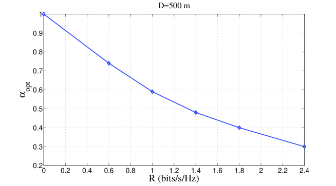
Figure 4: Optimal reuse factor vs. average rate of a sector

In Figure 4, we plot $\alpha_{\textrm{opt}}$ defined by (31) for different values of the average rate $\bar{R}$. As expected, $\alpha_{\textrm{opt}}$ is decreasing with respect to $\bar{R}$. Indeed, the larger the value $\bar{R}$, the higher the level of interference, and the greater the number of users that should be assigned protected subcarriers.

Selection of separating curves $\boldsymbol{\{d_{\textrm{subopt}}^{c}(.)\}_{c=A,B,C}}$

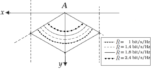
Figure 5: Optimal separating curve $d_{\theta^{A}}(.)$

Once the reuse factor is set to the value $\alpha_{\textrm{opt}}$, the separating curves $\{d_{\textrm{subopt}}^{c}(.)\}_{c=A,B,C}$ associated with the proposed suboptimal allocation algorithm should be chosen to be equal to the asymptotic optimal curves $\{d_{\theta^{c}}(.)\}_{c=A,B,C}$ given by Lemma 4. Since we are considering the case where the asymptotic distribution of users is the same in the three sectors, Algorithm 4 yielded in all our simulations three identical separating curves i.e., for all $x\in[-D,D]$, $d_{\textrm{subopt}}^{A}(x)=d_{\textrm{subopt}}^{B}(x)=d_{\textrm{subopt}}^{C}(x)$. Figure 5 plots $d_{\textrm{subopt}}^{A}(.)$ for different values of the average rate $\bar{R}$.

Performance of the proposed allocation algorithm

From now on, the positions of users in each sector are assumed to be uniformly distributed random variables. We also assume that all users have the same target rate, and that $K^{A}=K^{B}=K^{C}$. In the sequel, $r_{T}=\sum_{k=1}^{K^{c}}r_{k}$ designates the sum rate per sector measured in bits/s. Let us study the performance of the proposed allocation algorithm (Algorithm 3) in the case where the separating curves $\{d_{\textrm{subopt}}^{c}(.)\}_{c=A,B,C}$ are selected as in Subsection V-B (see Figure 5).

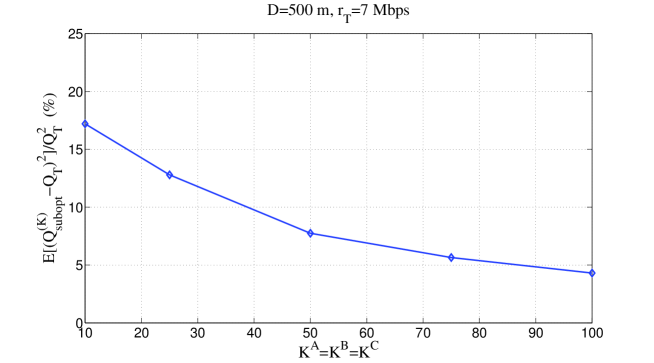
Figure 6: $\mathbb{E}\left(Q_{\textrm{subopt}}^{(K)}-Q_{T}\right)^{2}/Q_{T}^{2}$ vs. number of users per sector

We first validate the asymptotic optimality of Algorithm 3. To that end, we consider 5 values of the number $K$ of users comprised between 30 and 300. For each one of these values, the system bandwidth $B=B(K)$ is chosen such that $K/B=t=15\times 10^{-6}$. For example, the bandwidth is equal to 5 MHz when $K=75$ i.e., when $K^{A}=K^{B}=K^{C}=25$. This way, the number of users increases in accordance with the description of the asymptotic regime given earlier in Section V-A. Next, we compute the transmit powers $Q_{\textrm{subopt}}^{(K)}$ spent when Algorithm 3 is applied for a large number of realizations of the random positions of users. We finally evaluate the associated mean value $\mathbb{E}\left[Q_{\textrm{subopt}}^{(K)}\right]$ (expectation is taken w.r.t the random positions of users) and compare it with the asymptotic optimal transmit power $Q_{T}=\lim_{K\to\infty}Q_{T}^{(K)}$ as given by Lemma 4. The results of this comparison are illustrated in Figure 6. Note that the difference between $Q_{\textrm{subopt}}^{(K)}$ and $Q_{T}$ decreases with the number of users. This difference can be considered negligible even for a moderate number of users equal to 50 per sector. This sustains that the proposed allocation algorithm is asymptotically optimal.

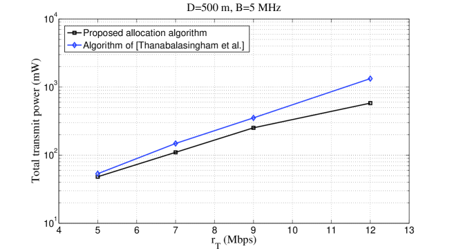
Figure 7: Comparison between the proposed allocation algorithm and the scheme of [23] for $K^{A}=K^{B}=K^{C}=25$

From now on, the system bandwidth $B$ is equal to 5 MHz and the number of users per sector is fixed to 25. In Figure 7, we compare the proposed algorithm with the allocation scheme introduced in [23]. In the latter work, the authors set the value of the reuse factor $\alpha$ to one i.e., all the available subcarriers are reused in all the cells. The resource allocation problem they address consists (as in our paper) in minimizing the total power that should be spent by the network in order to achieve all users’ rate requirements. In this context, they propose a distributed iterative allocation algorithm similar to Algorithm 1. The main difference is that, while Algorithm 1 is only applied to a subset $\mathcal{K}_{I}^{A}\cup\mathcal{K}_{I}^{B}\cup\mathcal{K}_{I}^{C}$ of users, the algorithm of [23] is applied to all the users in the network. As a matter of fact, this difference has no significant effect on the computational complexity of the scheme of [23], which is also of order $O(N_{\textrm{iter}}N_{\textrm{grad}}K)$ as Algorithm 1 (see Subsection IV-D). However, Figure 7 shows that for all the different values of the sum rate $r_{T}$, considerable gains can be achieved by applying our resource allocation scheme instead of that of [23] without any additional computational complexity.

Convergence rate of Algorithm 1

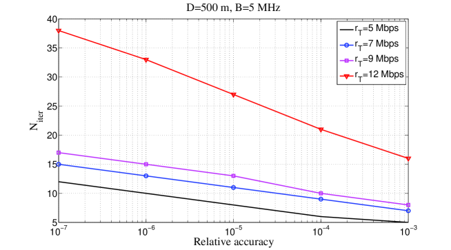
Figure 8: Number of iterations of Algorithm 1 vs. relative accuracy

We plot in Figure 8 the number $N_{\textrm{iter}}$ of iterations of Algorithm 1 as a function of the required accuracy i.e., the maximum relative change in the transmit powers $Q_{1}^{c}$ ($c=A,B,C$) from iteration to another beyond which convergence of the algorithm is achieved. Figure 8 shows that Algorithm 1 converges quickly within a very good accuracy even for a sum rate as high as 9 Mbps.

Performance of the proposed allocation algorithm in the discrete case

We now address the so-called discrete case where the sharing factors should be integer multiples of $1/N$. In this context, we propose the following approach to compute the resource allocation parameters. We first apply Algorithm 3 to obtain the continuous-valued sharing factors $\gamma_{k,1}^{c}$ and $\gamma_{k,2}^{c}$ for $c=A,B,C$. Next, we round the number of assigned subcarriers $\gamma_{k,1}^{c}N$ and $\gamma_{k,2}^{c}N$ to the nearest smaller integer. In order to compensate for the slight decrease of each sharing factor due to rounding, the power allocated to each user should be slightly increased so as to keep the same achievable rate. To that end, the power allocation should be recomputed (this time, keeping fixed sharing factors). This can be achieved by straightforward adaptation of Algorithms 1 and 2. In Figure 9, we plot the required transmit power in the discrete case assuming the following values of the total number $N$ of subcarriers: $N=72,192,360$ as recommended in WiMax [26]. Figure 9 shows that our allocation algorithm continues to do relatively well even after rounding the sharing factors, provided that the total number of subcarriers is moderately large enough.

Performance of the proposed allocation algorithm in larger networks

We now turn our attention to the 21-sector network of Figure 10. This network is composed of 7 duplicates of the 3-sector system of Figure 1. Note from Figure 10 that the subcarriers of subsets $\mathcal{P}_{A}$, $\mathcal{P}_{B}$, $\mathcal{P}_{C}$ are no more interference-free. However, the number of interferers for users modulating in these subsets is always smaller than the number of interferers for users modulating in subset $\mathcal{I}$.

In this context, we propose the following procedure. We first fix the separating curve $\{d_{\textrm{subopt}}^{c}(.)\}$ in each sector $c$ and the reuse factor $\alpha$ to the values given by Sections V-B and V-D respectively i.e., as if the network were composed of only three sectors. Note that Algorithm 2 cannot be applied anymore since the users outside the curves $\{d_{\textrm{subopt}}^{c}(.)\}$ are now subject to multicell interference. Instead, we apply a straightforward adaptation of Algorithm 1 to the case of more than three sectors. In Figure 11, we plot both the transmit power of the above proposed algorithm and that of the distributed and iterative allocation scheme of [23] (both averaged w.r.t the random positions of users) assuming a 21-sector setting. We note from Figure 11 that, while the scheme of [23] fails to converge for sum rates $r_{T}$ larger or equal to 9 Mbps, our allocation algorithm converges in all the considered cases. It furthermore results in considerably smaller transmit powers. However, comparing Figures 7 and 11 reveals that the transmit power of the proposed algorithm is significantly larger in the 21-sector setting than in the 3-sector setting. Reducing this gap requires a large amount of research and is out of the scope of this paper.

VII Conclusions

In this paper, we addressed the problem of resource allocation for the downlink of a sectorized OFDMA network assuming fractional frequency reuse and statistical CSI. In this context, we proposed a practical resource allocation algorithm that can be implemented in a distributed manner. The proposed algorithm divides users of each cell into two groups which are geographically separated by a fixed curve: Users of the first group are constrained to interference-free subcarriers, while users of the second are constrained to subcarriers subject to interference. If the aforementioned separating curves are relevantly chosen, then the transmit power of this simple algorithm tends, as the number of users grows to infinity, to the same limit as the minimal power required to satisfy all users’ rate requirements. Therefore, the simple scheme consisting in separating users beforehand into protected and non protected users is asymptotically optimal. This scheme is frequently used in cellular systems, but it has never been proved optimal in any sense to the best of our knowledge. Finally, we proposed a method to select a relevant value of the reuse factor. The determination of this factor is of great importance for the dimensioning of wireless networks.

Appendix A Proof of Lemma 3

Notations. In the sequel, $\mathbf{x}_{ABC}$ represents a vector of multicell allocation parameters such that ${\bf x}_{ABC}=[{{\bf x}_{A}}^{T},{{\bf x}_{B}}^{T},{{\bf x}_{B}}^{T}]^{T}$ where $\mathbf{x}_{A}=[(\mathbf{P}^{A})^{T},(\boldsymbol{\gamma}^{A})^{T}]^{T}$, $\mathbf{x}_{B}=[(\mathbf{P}^{B})^{T},(\boldsymbol{\gamma}^{B})^{T}]^{T}$ and $\mathbf{x}_{C}=[(\mathbf{P}^{C})^{T},(\boldsymbol{\gamma}^{C})^{T}]^{T}$, and where for each $c=A,B,C$, $\mathbf{P}^{c}=[P_{1,1}^{c},P_{1,2}^{c},\ldots,P_{K^{c},1}^{c},P_{K^{c},2}^{c}]^{T}$ and $\boldsymbol{\gamma}=[\gamma_{1,1}^{c},\gamma_{1,2}^{c},\ldots$, $\gamma_{K^{c},1}^{c}$, $\gamma_{K^{c},2}^{c}]^{T}$. We respectively denote by $Q_{1}(\mathbf{x}_{c})=\sum_{k}\gamma_{k,1}^{c}P_{k,1}^{c}$ and $Q_{2}(\mathbf{x}_{c})=\sum_{k}\gamma_{k,2}^{c}P_{k,2}^{c}$ the powers transmitted by base station $c$ in the interference subset $\cal I$ and in the protected subset ${\cal P}_{c}$. When resource allocation ${\bf x}_{ABC}$ is used, the total power transmitted by the network is equal to $Q({\bf x}_{ABC})=\sum_{c}Q_{1}(\mathbf{x}_{c})+Q_{2}(\mathbf{x}_{c})$. Recall that Problem 1 is nonconvex. It cannot be solved using classical convex optimization methods. Denote by ${\bf x}_{ABC}^{*}=[{{\bf x}_{A}^{*}}^{T},{{\bf x}_{B}^{*}}^{T},{{\bf x}_{C}^{*}}^{T}]^{T}$ any global solution to Problem 1.

Characterizing ${\bf x}_{ABC}^{*}$ via single cell results.

From ${\bf x}_{ABC}^{*}$ we construct a new vector ${\bf x}_{ABC}$ which is as well a global solution and which admits a “binary” form: for each cell $c$, $\gamma_{k,1}^{c}=0$ if $y_{k}>d_{\theta_{c}}(x_{k})$ and $\gamma_{k,2}^{c}=0$ if $y_{k}<d_{\theta_{c}}(x_{k})$, for a certain curve $d_{\theta_{c}}(.)$. For cell $A$, vector ${\bf x}_{A}$ is defined as a global solution to the single cell Problem 3 when

• the admissible nuisance constraint $\cal Q$ is set to ${\cal Q}=Q_{1}({\bf x}_{A}^{*})$,

• the gain-to-interference-plus-noise-ratio in subset $\cal I$ is set to $g_{k,1}=g_{k,1}\left(Q_{1}({\bf x}_{B}^{*}),Q_{1}({\bf x}_{C}^{*})\right)$.

Vectors ${\bf x}_{B}$ and ${\bf x}_{C}$ are defined similarly, by replacing $A$ by $B$ or $C$ in the above definition. Denote by ${\bf x}_{ABC}=[{{\bf x}_{A}}^{T},{{\bf x}_{B}}^{T},{{\bf x}_{C}}^{T}]^{T}$ the allocation obtained by the above procedure. The following claim holds.

Claim 1.

Resource allocation parameters ${\bf x}_{ABC}$ and ${\bf x}_{ABC}^{*}$ coincide: ${\bf x}_{ABC}={\bf x}_{ABC}^{*}$.

Proof.

It is straightforward to show that ${\bf x}_{ABC}$ is a feasible point for the joint multicell problem (Problem 1) in the sense that constraints $\bf C1$-$\bf C4$ of Problem 1 are met. This is the consequence of the low nuisance constraint $Q_{1}({\bf x}_{c})\leq Q_{1}({\bf x}_{c}^{*})$ which ensures that the interference which is produced by each base station when using the new allocation ${\bf x}_{ABC}$ is no bigger than the interference produced when the initial allocation ${\bf x}_{ABC}^{*}$ is used. Second, it is straightforward to show that ${\bf x}_{ABC}$ is a global solution to the multicell problem (Problem 1). Indeed, the power $Q_{1}(\mathbf{x}_{c})+Q_{2}(\mathbf{x}_{c})$ spent by base station $c$ is necessarily less than the initial power $Q_{1}(\mathbf{x}_{c}^{*})+Q_{2}(\mathbf{x}_{c}^{*})$ by definition of the minimization Problem 3. Thus $Q({\bf x}_{ABC})\leq Q({\bf x}_{ABC}^{*})$. Of course, as ${\bf x}_{ABC}^{*}$ has been chosen itself as a global minimum of $Q$, the latter inequality should hold with equality: $Q({\bf x}_{ABC})=Q({\bf x}_{ABC}^{*})$. Therefore, ${\bf x}_{ABC}^{*}$ and ${\bf x}_{ABC}$ are both global solutions to the multicell problem (Problem 1). As an immediate consequence, inequality $Q_{1}(\mathbf{x}_{c})+Q_{2}(\mathbf{x}_{c})\leq Q_{1}(\mathbf{x}_{c}^{*})+Q_{2}(\mathbf{x}_{c}^{*})$ holds with equality in all the three cells $c=A,B,C$:

$$Q_{1}(\mathbf{x}_{c})+Q_{2}(\mathbf{x}_{c})=Q_{1}(\mathbf{x}_{c}^{*})+Q_{2}(\mathbf{x}_{c}^{*})\>.$$ (32)

Clearly, ${\bf x}_{A}^{*}$ is a feasible point for Problem 3 when setting ${\cal Q}=Q_{1}({\bf x}_{A}^{*})$ and $g_{k,1}=g_{k,1}\big{(}Q_{1}({\bf x}_{B}^{*})$, $Q_{1}({\bf x}_{C}^{*})\big{)}$. Indeed constraint $\bf C6$ is equivalent to $Q_{1}({\bf x}_{A}^{*})\leq{\cal Q}$ and is trivially met (with equality) by definition of $\cal Q$. Since the objective function $Q_{1}(\mathbf{x}_{A}^{*})+Q_{2}(\mathbf{x}_{A}^{*})$ coincides with the global minimum as indicated by (32), ${\bf x}_{A}^{*}$ is a global minimum for the single cell Problem 3. By Lemma 2, this problem admits a unique global minimum ${\bf x}_{A}$. Therefore, ${\bf x}_{A}^{*}={\bf x}_{A}$. By similar arguments, ${\bf x}_{B}^{*}={\bf x}_{B}$ and ${\bf x}_{C}^{*}={\bf x}_{C}$. ∎

We thus conclude that any global solution ${\bf x}_{ABC}^{*}$ to the multicell Problem 1 satisfies equations (18), (19), where $g_{k,1}$ in the latter equations coincide with $g_{k,1}=g_{k,1}\left(Q_{1}({\bf x}_{\bar{c}}^{*}),Q_{1}({\bf x}_{\bar{\bar{c}}}^{*})\right)$, and where for each cell $c\in\{A,B,C\}$, $\bar{c}$ and $\bar{\bar{c}}$ denote the other two cells. The proof of Lemma 3 is thus complete.

Algorithm 1 Ping-pong algorithm for three interfering cells

  Initialization: $Q_{1}^{A}\leftarrow 0$, $Q_{1}^{B}\leftarrow 0$, $Q_{1}^{C}\leftarrow 0$

  repeat

     $(\beta_{1}^{A},Q_{1}^{A})\leftarrow$ Solve (7)-(8) for $c=A$

     $(\beta_{1}^{B},Q_{1}^{B})\leftarrow$ Solve (7)-(8) for $c=B$

     $(\beta_{1}^{C},Q_{1}^{C})\leftarrow$ Solve (7)-(8) for $c=C$

  until convergence

  for all $c=A,B,C$ do

     $\{\gamma_{k,1}^{c},P_{k,1}^{c}\}_{k\in\mathcal{K}_{I}^{c}}\leftarrow$ (4)-(5)

  end for

  return  $\{\gamma_{k,1}^{c},P_{k,1}^{c}\}_{c=A,B,C,\>k\in\mathcal{K}_{I}^{c}}$

Algorithm 2 Resource allocation for protected users

  for all $c=A,B,C$ do

     $\beta_{2}^{c}\leftarrow$ Solve (12)

     for all $k\in\mathcal{K}_{P}^{c}$ do

        $P_{k,2}^{c}\leftarrow$ (10)

        $\gamma_{k,2}^{c}\leftarrow$ (11)

     end for

  end for

  return  $\{\gamma_{k,2}^{c},P_{k,2}^{c}\}_{c=A,B,\>k\in\mathcal{K}_{P}^{c}}$

Algorithm 3 Proposed resource allocation algorithm

  for all $c=A,B,C$ do

     $\mathcal{K}_{P}^{c}\leftarrow\{k\in\{1\ldots K^{c}\}\>|\>y_{k}>d_{\textrm{subopt}}^{c}(x_{k})\}$

     $\mathcal{K}_{I}^{c}\leftarrow\{k\in\{1\ldots K^{c}\}\>|\>y_{k}\leq d_{\textrm{subopt}}^{c}(x_{k})\}$

  end for

  $\{\gamma_{k,1}^{c},P_{k,1}^{c}\}_{c=A,B,C,\>k\in\mathcal{K}_{I}^{c}}\leftarrow$ Algorithm 1

  $\{\gamma_{k,2}^{c},P_{k,2}^{c}\}_{c=A,B,c,\>k\in\mathcal{K}_{P}^{c}}\leftarrow$ Algorithm 2

  return  $\{\gamma_{k,1}^{c},P_{k,1}^{c},\gamma_{k,2}^{c},P_{k,2}^{c}\}_{c=A,B,C,\>k=1\ldots K^{c}}$

Algorithm 4 Determination of $\{\theta^{c}\}_{c=A,B,C}$

  for all $(Q_{1}^{A},Q_{1}^{B},Q_{1}^{C})$ do

     for $c=A,B,C$ do

        if (24)-(28)-(29) admits a solution then

           $(\beta_{1}^{c},\beta_{2}^{c},\xi^{c})\leftarrow$ unique solution to (24)-(28)-(29)

           $\theta^{c}\leftarrow(\beta_{1}^{c},\beta_{2}^{c},Q_{1}^{\bar{c}},Q_{1}^{\bar{\bar{c}}},\xi^{c})$

           $Q^{c}\leftarrow Q_{1}^{c}+{\bar{R}}^{c}\int_{-D}^{D}\int_{d_{\theta^{c}}(x)}^{\frac{2D-|x|}{\sqrt{3}}}{\cal F}(x,y,\beta_{2}^{c},0,0,0)\>d\lambda^{c}(x,y)$

        else

           $Q^{c}\leftarrow\infty$

        end if

     end for

     $Q_{T}(Q_{1}^{A},Q_{1}^{B},Q_{1}^{C})\leftarrow\sum_{c=A,B,C}Q^{c}$

  end for

  $(Q_{1}^{A},Q_{1}^{B},Q_{1}^{C})\leftarrow\arg\min_{(\tilde{Q}_{1}^{A},\tilde{Q}_{1}^{B},\tilde{Q}_{1}^{C})}Q_{T}(\tilde{Q}_{1}^{A},\tilde{Q}_{1}^{B},\tilde{Q}_{1}^{C})$

  for $c=A,B,C$ do

     $\theta^{c}\leftarrow(\beta_{1}^{c},\beta_{2}^{c},Q_{1}^{\bar{c}},Q_{1}^{\bar{\bar{c}}},\xi^{c})$

  end for

  return  $\theta^{A},\theta^{B},\theta^{C}$

Figure 9: Transmit power of the proposed algorithm in case the sharing factors are integer multiples of $1/N$

Figure 10: 21-sector system model and the frequency reuse scheme

Figure 11: Comparison between the proposed allocation algorithm and the scheme of [23] in the case of 21 sectors for $K^{c}=25$

References

- [1] K. Seong, M. Mohseni and J. M. Cioffi, Optimal resource allocation for OFDMA downlink systems, ISIT, Jul. 2006.
- [2] F. Brah, L. Vandendorpe and J. Louveaux, Constrained resource allocation in OFDMA downlink systems with partial CSIT, ICC , May, 2008.
- [3] I.C. Wong and B.L. Evans, Optimal resource allocation in OFDMA systems with imperfect channel knowledge, IEEE Transaction on Communications, vol. 57, no. 1, Jan. 2009.
- [4] M. Ergen, S. Coleri and P. Varaiya, QoS aware adaptive resource allocation techniques for fair scheduling in OFDMA based broadband wireless access systems, IEEE Transactions on Broadcasting, vol. 49, no. 4, dec. 2003.
- [5] C. Y. Wong, R. S. Cheng, K. Ben Letaief and R. D. Murch, Multiuser OFDM with adaptive subcarrier, bit and power allocation, IEEE Journal on Selected Areas in Communications, vol. 17, num. 10, sep. 1999.
- [6] D. Kivanc, G. Li and H. Liu, Computationally efficient bandwidth allocation and power control for OFDMA, IEEE Transactions on Wireless Communications, vol. 2, no. 6, nov. 2003.
- [7] D. Gesbert, M. Kountouris, Joint power control and user scheduling in multi-cell wireless networks: Capacity scaling Laws, submitted to IEEE Transactions On Information Theory, September 2007.
- [8] M. Pischella and J.-C. Belfiore, Distributed resource allocation for rate-constrained users in multi-cell OFDMA networks, IEEE Communications Letters, vol. 12, no. 4, April, 2008.
- [9] E. Jorswieck and R. Mochaourab, Power control game in protected and shared bands: Manipulability of Nash equilibrium, International Conference on Game Theory for Networks (GameNets’09), May 2009, Invited.
- [10] C. Lengoumbi, Ph. Godlewski and Ph. Martins, Dynamic subcarrier reuse with rate guaranty in a downlink multicell OFDMA system, IEEE International Symposium on Personal, Indoor and Mobile Radio Communications, 2006.
- [11] S. Hammouda, S. Tabbane and Ph. Godlewski, Improved reuse partitioning and power control for downlink multi-cell OFDMA systems, International Workshop on Broadband Wireless Access for ubiquitous Networking, September, 2006.
- [12] M. Pischella and J.-C. Belfiore, Distributed resource allocation in MIMO OFDMA networks with statistical CSIT, SPAWC, June, 2009.
- [13] S. Gault and W. Hachem and P. Ciblat, Performance analysis of an OFDMA transmission system in a multi-cell environment, IEEE Transactions on Communications, num. 12, vol. 55, pp. 2143-2159, December, 2005.
- [14] WiMAX Forum, Mobile WiMAX - Part II: A comparative analysis, available at http://www.wimaxforum.org/.
- [15] IEEE 802.16-2004, Part 16: Air interface for fixed broadband wireless access systems, IEEE Standard for Local and Metropolitan Area Networks, Oct. 2004.
- [16] A. Dotzler, G. Dietl and W. Utschick, Fractional reuse partitioning for MIMO networks, Accepted for Presentation at the 29th IEEE Global Telecommunications Conference (GLOBECOM 2010), Miami, Florida, USA, Dec. 2010.
- [17] A.L. Stolyar and H. Viswanathan, Self-organizing dynamic fractional frequency reuse in OFDMA systems, In Proceedings of the IEEE 27th Conference on Computer Communications (INFOCOM’2009), June 2008.
- [18] R. Ghaffar, R. Knopp, Fractional Frequency Reuse and Interference Suppression for OFDMA Networks, 8th International Symposium on Modeling and Optimization in Mobile, Ad Hoc, and Wireless Networks (WiOpt’10), Avignon, France, June 2010.
- [19] N. Ksairi, P. Bianchi, P. Ciblat and W. Hachem, Resource allocation for downlink cellular OFDMA systems: Part I—Optimal allocation, IEEE Transactions on Signal Processing, vol. 58, no. 2, Feb. 2010.
- [20] N. Ksairi, P. Bianchi, P. Ciblat and W. Hachem, Resource allocation for downlink cellular OFDMA systems: Part II—Practical algorithms and optimal reuse factor, IEEE Transactions on Signal Processing, vol. 58, no. 2, Feb. 2010.
- [21] IEEE Std. 802.16a: IEEE Standard for local and metropolitan area networks, Part 16: Air Interface for Fixed Broadband Wireless Access Systems-Amendment 2: Medium Access Control Modifications and Additional Physical Layer Specifications for 2-11 GHz, 2003.
- [22] N. Ksairi, Some resource allocation and cooperation techniques for future wireless communication systems, PHD Thesis, available at http://perso.telecom-paristech.fr/~bianchi/nassar.pdf.
- [23] T. Thanabalasingham, S. V. Hanly, L. L. H. Andrew and J. Papandriopoulos, Joint allocation of subcarriers and transmit powers in a multiuser OFDM cellular network, IEEE International Conference on Communications ICC, vol. 1, June 2006.
- [24] R. D. Yates, A framework for uplink Power control in cellular radio systems, IEEE Journal on Selected Areas in Communications, vol. 13, no. 7, September 1995.
- [25] S. Boyd and L. Vandenberghe, Convex optimization, Cambridge University Press, 2004.
- [26] J. G. Andrews, A. Ghosh and R. Uhamed, Fundamentals of WiMax: Understanding broadband wireless networking, Prentice Hall, 2007.