Regularized Sampling of Multiband Signals

Abstract

This paper presents a regularized sampling method for multiband signals, that makes it possible to approach the Landau limit, while keeping the sensitivity to noise at a low level. The method is based on band-limited windowing, followed by trigonometric approximation in consecutive time intervals. The key point is that the trigonometric approximation “inherits” the multiband property, that is, its coefficients are formed by bursts of non-zero elements corresponding to the multiband components. It is shown that this method can be well combined with the recently proposed synchronous multi-rate sampling (SMRS) scheme, given that the resulting linear system is sparse and formed by ones and zeroes. The proposed method allows one to trade sampling efficiency for noise sensitivity, and is specially well suited for bounded signals with unbounded energy like those in communications, navigation, audio systems, etc. Besides, it is also applicable to finite energy signals and periodic band-limited signals (trigonometric polynomials). The paper includes a subspace method for blindly estimating the support of the multiband signal as well as its components, and the results are validated through several numerical examples.

I Introduction

Sampling is the operation that makes the discrete processing of continuous signals possible. The basic tool for this operation is Shannon’s Sampling Theorem, which states that a signal can be reconstructed without error from its samples taken at a rate equal to twice its maximum frequency (Nyquist rate), [1]. In some situations, however, the signal is multiband, in the sense that its spectral support is composed of a finite set of disjoint intervals. In this case, sampling at the Nyquist rate can be very inefficient. The design of alternative sampling schemes for this kind of signals has been an active research topic for decades. It was first demonstrated by H. J. Landau in [2] that if the signal is sampled nonuniformly, then the average sampling rate is lower bounded by the measure of its spectral support, (Landau lower bound). Later, it was shown in [3] that there exist nonuniform sampling patterns that approach this bound as much as desired. The sampling scheme in this reference was the so-called “multi-coset sampling”, which consists in selecting a sampling rate above the Nyquist rate, and then choosing a periodic nonuniform subsequence of it. The subsequent investigations on this topic have mainly focused on devising low complexity and stable (low sensitivity) implementations of multi-coset sampling, [4, 5, 6, 7]. Recently, compressed sensing techniques have been applied to multi-coset sampling in [8, 9], so as to detect the band positions, as well as to reconstruct each of the components. An alternative method to discretize multiband signals is the random demodulator in [10, 11], in which the complexity of the analog processing is increased, with the aim of employing only analog-to-digital converters of moderate input bandwidth. Finally, it is worth mentioning the synchronous multi-rate sampling (SMRS) scheme in [12]. Here, the multiband signal is sampled in several uniform grids with different rates, in order to produce a bunch of lowpass signals, in which the spectrum of the multiband signal appears aliased. The key idea is that this aliasing may not affect all frequencies of the original spectral support for all sampling rates. This fact is exploited in [12] by properly selecting the number of sampling frequencies, so as to achieve the reconstruction of the multiband signal. This technique has been further developed in a second paper, which also includes the application of compressed sensing [13].

An assumption that is common to these approaches is that of finite energy: the multiband components are assumed to be in the Lebesgue space $L^{2}$, and the machinery of Fourier analysis for this space is applied extensively. This way to proceed simplifies the analysis, because signals in $L^{2}$ have a proper spectrum function, and the well-known properties of the Fourier transform apply. Nevertheless, there is a mismatch between this model and the situation encountered in multitude applications, (communications, audio, navigation, etc). Quite often, it is not possible to sample a time interval that contains most of the signal’s energy due to its long duration. This limitation has negative effects, that can be readily noticed in the single-band case by analyzing the Sampling Theorem. Given a finite energy signal ${\mathrm{s}}(t)$ whose spectrum lies in $[-1/(2\tau),1/(2\tau)]$, the Sampling Theorem provides the representation

$${\mathrm{s}}(n\tau+u)=\sum_{p=-\infty}^{\infty}{\mathrm{s}}((n-p)\tau){\mathrm{sinc}}(p+u/\tau),$$ (1)

where $n$ is an integer and $u$ is any time shift following $-\tau/2\leq u<\tau/2$. Yet in practice, the infinite set of samples ${\mathrm{s}}((n-p)\tau)$ is not available, and then (1) must be truncated at some index $P$

$${\mathrm{s}}(n\tau+u)\approx\sum_{p=-P}^{P}{\mathrm{s}}((n-p)\tau){\mathrm{sinc}}(p+u/\tau).$$ (2)

This last formula is well known for its poor accuracy, [14]. The problem lies in that (1) converge only because the samples ${\mathrm{s}}((n-p)\tau)$ converge to zero as $|p|\rightarrow\infty$, due to the fact that ${\mathrm{s}}(t)$ has finite energy. So, if the energy of ${\mathrm{s}}(t)$ is mostly outside the sampling interval $[-PT,PT]$, the accuracy is poor due to the sinc tails corresponding to the neglected samples.

This problem is well known in the signal processing field, and it can be solved by regularizing the interpolation formula in (2), using various filter design techniques, [15]. A typical method consists in assuming that there is some excess sampling bandwidth, i.e, that the spectrum of ${\mathrm{s}}(t)$ lies in $[-B/2,B/2]$ with $B\tau<1$ (and not $B\tau\leq 1$), and then multiplying the sinc samples in (2) by a set of weights ${\mathrm{v}}_{p}(u)$,

$${\mathrm{s}}(n\tau+u)\approx\sum_{p=-P}^{P}{\mathrm{s}}((n-p)\tau){\mathrm{v}}_{p}(u){\mathrm{sinc}}(p+u/\tau).$$ (3)

This regularization converts the ill-behaved interpolator in (2) into a well-behaved one, and this can be readily seen in the error trends: while the interpolation error of (2) decreases only as $1/P$, [14], there are sets of coefficients ${\mathrm{v}}_{p}(u)$ for which the error of (3) decreases exponentially as ${\mathrm{e}}^{-\pi(1-B\tau)P}$, [20]. The price paid for the regularization is that it is not possible to represent signals using the full sampling bandwidth anymore, and it is also not possible to implement filters with sharp transitions, since this would produce convergence problems similar to those of the sinc series.

By analogy with the single band case, the multiband problem is currently in the stage equivalent to that of the sinc series in (1) and its truncated version in (2); i.e, some sampling schemes have been identified that approach the Landau rate, and allow the recovery of the multiband signal and its components, but there is no regularization procedure available. This lack of regularization can be noticed in analytical devices, like the slicing of the spectrum using sharp transitions, and in the use of discrete sequences with full spectrum, like coset sequences.

The purpose of this paper is to present a regularized sampling scheme for multiband signals. Relative to the existing methods in the literature, the one in this paper provides a flexible interface between the multiband signal and its discrete representation, that allows one to trade sampling efficiency for noise sensitivity. In the scheme, the reconstruction procedure is specified in the form of weighted trigonometric polynomials, which are able to interpolate the multiband signal and its components in consecutive time intervals.

The starting point in the derivation of the scheme is the boundness assumption which substitutes the usual finite energy assumption, i.e, the multiband components are assumed to have bounded time amplitude, but their energy can be unlimited. To make no assumption about the energy is meaningful since, for long signals, it usually lies outside the sampling interval and can be arbitrarily large. And to work assuming bounded components reflects clear physical and engineering constraints: signals have bounded peak power due to restrictions like the maximum transmitted power, or due to systems like automatic gain controls. With the new assumption, the multiband components have a lowpass equivalent whose real and imaginary parts belong to the Bernstein space $\mathcal{B}_{\pi B}^{\infty}$, [16, chapter 6], i. e, they can be described as entire functions of exponential type that are real and bounded on the real axis. This new description has the drawback that the basic tool in spectral analysis, namely the Fourier transform (Plancherel theorem), is not directly usable. So, basic analytic procedures in the literature on multiband sampling [3, 12, 13, 17, 10, 11], like the division of the spectrum in disjoint intervals, the use of discrete sequences with full spectrum (like coset sequences), and the use of lowpass filters with sharp transitions are not valid on bounded band-limited signals. However, these tools can be substituted by a simple yet powerful analytical device, as shown in this paper. If ${\mathrm{z}}(t)$ is the multiband signal, the device consists in multiplying ${\mathrm{z}}(t)$ by a bandlimited window ${\mathrm{w}}(t)$, that approximately “selects” a given finite interval, in the sense that its $L^{1}$ time-domain content is concentrated in it. The key result is that there exist windows ${\mathrm{w}}(t)$, for which the product ${\mathrm{z}}(t){\mathrm{w}}(t)$ is a trigonometric polynomial with negligible error in the interval selected by ${\mathrm{w}}(t)$. Besides, the trigonometric polynomial “inherits” the multiband structure of ${\mathrm{z}}(t)$, i.e, its coefficients are formed by bursts of values corresponding to the bands of ${\mathrm{z}}(t)$. Sec. III is dedicated to this analytical device.

After this, the design of a sampling scheme is addressed in Sec. IV, where it is designed for sparse trigonometric polynomials, since the product ${\mathrm{z}}(t){\mathrm{w}}(t)$ can be viewed as a polynomial of this type with negligible error. In this section, it is shown that a finite version of the SMRS scheme produces a sparse linear system, in which the sensitivity to noise can be reduced by increasing the number of samples. Afterward, Sec. V shows how the finite sampling grid for ${\mathrm{z}}(t){\mathrm{w}}(t)$ can exactly match an infinite SMRS scheme for ${\mathrm{z}}(t)$. This makes it possible to interpolate ${\mathrm{z}}(t)$ and its components at any $t$. The interpolation error is then analyzed in Sec. VI. Finally, the blind sampling problem is studied in Sec. VII, where the MUSIC algorithm from direction of arrival estimation is adopted.

Since the notation in the paper is extensive, the basic symbols and operators are described in the next sub-section, and there is a list of symbols at the end of the paper in Table I. The next section sketches the sampling method, in order to give a broad view of the concepts involved. The novel aspects of the paper are, fundamentally, the contents of Secs. III to V and Sec. VII.

I-A Notation

Several conventions have been adopted in the paper to simplify the notation:

• Definitions are performed using the operator “$\equiv$”.

• $R(\tau,T)$ denotes the interval

  $$R(\tau,T)\equiv[\tau-T/2,\tau+T/2[$$ (4)

  for arbitrary $\tau$ and $T>0$.

• The symbols $J$, $J^{\prime}$, $I_{zw}$ and $I_{sw,m}$ denote sets of distinct indices (integers). In $I_{zw}$ and $I_{sw,m}$ the subscripts ’$zw$’ and ’$sw$’ remind one of the meaning of these sets: thus, $I_{zw}$ and $I_{sw,m}$ are the index sets of ${\mathrm{z}}(t)$ and ${\mathrm{s}}_{m}(t)$, respectively, after windowing using ${\mathrm{w}}(t)$.

• $|J|$ denotes the number of elements of a set $J$.

• The operator “$\tilde{\;\;\;}$” denotes periodization with period $T$, that is, for a signal ${\mathrm{s}}(t)$, it is

  $$\tilde{{\mathrm{s}}}(t)\equiv\sum_{p=-\infty}^{\infty}{\mathrm{s}}(t+pT).$$ (5)

• Vectors and matrices are written in bold font and in lower and upper case, respectively, ($\mathbf{m}$, $\mathbf{M}$).

• $\mathbf{I}$ denotes the identity matrix.

• $[\mbox{\boldmath$\mathbf{A}$\unboldmath}]_{h,n}$ denotes the $h,n$ element of matrix $\mathbf{A}$; ${[}\mbox{\boldmath$\mathbf{p}$\unboldmath}]_{r}$ denotes the $r$-th element of vector $\mathbf{p}$; and $[\mbox{\boldmath$\mathbf{A}$\unboldmath}]_{\cdot,n}$ the $n$-th column of a matrix $\mathbf{A}$.

II Sketch of the proposed method

Consider a multiband signal ${\mathrm{z}}(t)$ formed by $M$ bounded band-limited components ${\mathrm{s}}_{m}(t)$,

$${\mathrm{z}}(t)=\sum_{m=1}^{M}{\mathrm{s}}_{m}(t),$$ (6)

where the band of ${\mathrm{s}}_{m}(t)$ is $[a_{m},b_{m}]$, and these bands are known and appear in increasing order, $b_{m}<a_{m+1}$, $m=1,\ldots,M-1$. The $m$-th component can be viewed as a signal whose baseband version

$${\mathrm{s}}_{m}(t){\mathrm{e}}^{-j\pi(a_{m}+b_{m})t}$$ (7)

has real and imaginary parts in the space $\mathcal{B}_{\pi(b_{m}-a_{m})}^{\infty}$. The spectral support of ${\mathrm{z}}(t)$ is the set

$$\mathcal{S}_{z}\equiv\bigcup_{m=1}^{M}[a_{m},b_{m}].$$ (8)

The multiband sampling problem can be posed in a finite time interval, centered at an arbitrary instant $\tau$, $R(\tau,T)$, $T>0$, in which a set of samples is taken at distinct instants $\tau+t_{1},\tau+t_{2},\ldots,\tau+t_{N}$, but assuming that the components ${\mathrm{s}}_{m}(t)$ must be interpolated only inside a shorter interval $R(\tau,T_{1})$, $T_{1}<T$. The objective is then to find a set of functions ${\mathrm{h}}_{m,n}(t)$, such that the components ${\mathrm{s}}_{m}(t)$ and ${\mathrm{z}}(t)$ can be interpolated using

$${\mathrm{s}}_{m}(\tau+t)\approx\sum_{n=1}^{N}{\mathrm{z}}(\tau+t_{n}){\mathrm{h}}_{m,n}(t)$$ (9)

and

$${\mathrm{z}}(\tau+t)\approx\sum_{m=1}^{M}\sum_{n=1}^{N}{\mathrm{z}}(\tau+t_{n}){\mathrm{h}}_{m,n}(t),$$ (10)

for $t$ in $R(0,T_{1})$. If there is a method to solve this last problem, then it can be applied repeatedly in overlapping intervals $R(\tau+kT_{1},T)$ with integer $k$, so as to interpolate ${\mathrm{z}}(t)$ and the components ${\mathrm{s}}_{m}(t)$ at any $t$. So, for example, the value of any of the components ${\mathrm{s}}_{m}(t)$ in a regular grid of instants $n\Delta t$, with integer $n$ and arbitrary $\Delta t>0$, could be obtained by evaluating (9) in the intersection of this grid with $R(\tau+kT_{1},T)$, and repeating the procedure for consecutive values of $k$.

In this setting, consider a band-limited window ${\mathrm{w}}(t)$ with spectrum lying in $[-B_{w}/2,B_{w}/2]$, $B_{w}>0$, that is approximately time limited to the interval $R(0,T)$. Besides, assume that it is bounded between one and a minimum value greater than zero in $R(0,T_{1})$, that is, $\delta_{w}\leq{\mathrm{w}}(t)\leq 1$ in $R(0,T_{1})$, $\delta_{w}>0$. Note that ${\mathrm{w}}(t)$ is not the typical window in filter design, that sharply selects a given time interval and nulls the rest of the time axis. Actually, it is the dual case: the spectrum of ${\mathrm{w}}(t)$ sharply selects the band $[-B_{w}/2,B_{w}/2]$, and ${\mathrm{w}}(t)$ is very small but not strictly zero outside $R(0,T)$. If $B_{w}$ is smaller than the minimum separation among bands of ${\mathrm{z}}(t)$,

$$B_{w}<\min_{m}a_{m+1}-b_{m},\;\;m=1,\ldots,M-1,$$ (11)

then the product ${\mathrm{z}}(\tau+t){\mathrm{w}}(t)$ is also a multiband signal with components ${\mathrm{s}}_{m}(\tau+t){\mathrm{w}}(t)$,

$${\mathrm{z}}(\tau+t){\mathrm{w}}(t)=\sum_{m=1}^{M}{\mathrm{s}}_{m}(\tau+t){\mathrm{w}}(t),$$ (12)

and spectral support

$$\mathcal{S}_{zw}\equiv\bigcup_{m=1}^{M}[a_{m}-B_{w}/2,b_{m}+B_{w}/2].$$ (13)

Thus, ${\mathrm{z}}(\tau+t){\mathrm{w}}(t)$ is another multiband signal in which the bands of ${\mathrm{z}}(t)$ have been expanded, but are still disjoint due to (11). Now, the multiband sampling problem can be posed in (12) with sampling instants $t_{n}$ and sample values ${\mathrm{z}}(\tau+t_{n}){\mathrm{w}}(t_{n})$. If there is a satisfactory solution for this last problem, then the original multiband signal ${\mathrm{z}}(t)$ and its components ${\mathrm{s}}_{m}(t)$ can be readily interpolated in $R(\tau,T_{1})$, simply by dividing by ${\mathrm{w}}(t)$.

In the windowed model in (12), the signal ${\mathrm{z}}(\tau+t){\mathrm{w}}(t)$ is approximately time-limited. This allows one to apply the Sampling Theorem, but with the time and frequency domains switched, i.e, ${\mathrm{z}}(\tau+t){\mathrm{w}}(t)$ is repeated periodically with period $T$ in the time domain, and this operation samples the frequency domain. Here, the window ${\mathrm{w}}(t)$ acts as a time-domain “lowpass filter” with nonuniform response. The result of this operation is a trigonometric polynomial, with coefficients equal to samples of the spectrum of ${\mathrm{z}}(\tau+t){\mathrm{w}}(t)$, taken at the frequencies $p/T$ with integer $p$, that lie in (13). If $I_{sw,m}$ denotes the integer indices $p$ of the frequencies $p/T$ inside the band of ${\mathrm{s}}_{m}(\tau+t){\mathrm{w}}(t)$,

$$I_{sw,m}\equiv\{p:a_{m}-B_{w}/2\leq p/T\leq b_{m}+B_{w}/2,p\in\mathbb{Z}\},$$ (14)

and $I_{zw}$ denotes the union of these sets,

$$I_{zw}\equiv\bigcup_{m=1}^{M}I_{sw,m},$$ (15)

then this approximate sampling theorem says that ${\mathrm{z}}(\tau+t){\mathrm{w}}(t)$ is the polynomial

$${\mathrm{z}}(\tau+t){\mathrm{w}}(t)\approx\sum_{p\in I_{zw}}{\mathrm{c}}_{p}(\tau){\mathrm{e}}^{j2\pi pt/T},$$ (16)

for $t$ in $R(0,T)$, where the ${\mathrm{c}}_{p}(\tau)$ are unknown samples of the spectrum of ${\mathrm{z}}(\tau+t){\mathrm{w}}(t)$. Besides, the components ${\mathrm{s}}_{m}(t)$ can be interpolated using

$${\mathrm{s}}_{m}(\tau+t)\approx\frac{1}{{\mathrm{w}}(t)}\sum_{p\in I_{sw,m}}{\mathrm{c}}_{p}(\tau){\mathrm{e}}^{j2\pi pt/T},$$ (17)

for $t$ in $R(0,T_{1})$.

As will be shown in this paper, the accuracy of this approximation depends on the window ${\mathrm{w}}(t)$. Actually, it is shown in the next section that the interpolation error is bounded by $A_{z}\epsilon/\delta_{w}$, where $A_{z}$ is a bound on the amplitude of ${\mathrm{z}}(t)$, and $\epsilon$ a bound on the summation

$$\sum_{|p|\neq 0}|{\mathrm{w}}(t+pT)|\leq\epsilon,\;\;t\;\mathrm{in}\;R(0,T).$$ (18)

The fact is that there exist windows, as the one presented in this paper, for which $\delta_{w}$ grows with $T$, and $\epsilon$ decreases exponentially as $T\rightarrow\infty$ with trend roughly equal to ${\mathrm{e}}^{-\pi B_{w}T}$. Thus, there is a moderate value of $T$ for fixed $B_{w}$ such that (17) can be regarded as an equality, for any fixed numerical precision. There are several methods to construct this kind of window, [18, 19, 20]. The one proposed in this paper in Sec. III-A is based on the properties of the Fourier transform of the Kaiser-Bessel function. Fig. 1 shows this kind of interpolation for a baseband BPSK signal ${\mathrm{s}}(t)$ using the window in this paper. The bold curve is the windowed signal, that is selected for $\epsilon=10^{-8}$ in (18). Fig. 2 shows the interpolation error, which is below -200 dB roughly in $R(0,T/2)$. (For details, see Sec. VIII-A.)

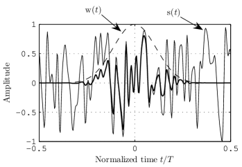
Figure 1: BPSK signal (bandwidth $136/T$, roll off $0.8$, chip rate $0.01324T$), window ${\mathrm{w}}(t)$ ($B_{w}T=13.6$), and windowed signal (bold curve) in Sec. VIII-A.

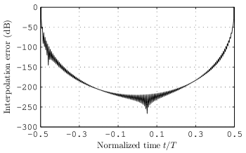
Figure 2: Interpolation error in validation of the interpolation method in Sec. VIII-A.

Coming back to the formula in (16), if $\epsilon$ is sufficiently small, then ${\mathrm{z}}(\tau+t){\mathrm{w}}(t)$ can be regarded as a trigonometric polynomial. This implies that the windowed problem in Eq. (12) can be cast in a generic setting, as that of computing the coefficients $\beta_{p}$ of a sparse trigonometric polynomial from its samples at the abscissas $t_{1},t_{2},\ldots,t_{N}$. If $J$ is an index set, then this kind of polynomial can be expressed as

$${\mathrm{\alpha}}(t;J)\equiv\sum_{p\in J}\beta_{p}{\mathrm{e}}^{j2\pi pt/T}.$$ (19)

The polynomial on the right in (16) has this form with $J=I_{zw}$ and $\beta_{p}={\mathrm{c}}_{p}(\tau)$. In this generic setting, the sampling problem reduces to solving the linear system

$${\mathrm{\alpha}}(t_{n};J)\equiv\sum_{p\in J}\beta_{p}{\mathrm{e}}^{j2\pi pt_{n}/T},\;\;n=1,\ldots,N.$$ (20)

If this system has full column rank, then the coefficients $\beta_{p}$ can be obtained using

$$\beta_{p}=\sum_{n=1}^{N}\eta_{p,n}{\mathrm{\alpha}}(t_{n};J),$$ (21)

where $\eta_{p,n}$ denotes the pseudo-inverse of (20). Then, the solution of the sampling problem for ${\mathrm{\alpha}}(t;J)$ is obtained by substituting this last equation into (19). This yields

$${\mathrm{\alpha}}(t;J)=\sum_{n=1}^{N}{\mathrm{\alpha}}(t_{n};J){\mathrm{\theta}}_{n}(t;J)$$ (22)

where

$${\mathrm{\theta}}_{n}(t;J)\equiv\sum_{p\in J}\eta_{p,n}{\mathrm{e}}^{j2\pi pt/T}.$$ (23)

Besides, since any “component” of ${\mathrm{\alpha}}(t;J)$ is specified by a subset $J^{\prime}$, $J^{\prime}\subset J$, its associated sampling formula is obtained by replacing ${\mathrm{\theta}}_{n}(t;J)$ with ${\mathrm{\theta}}_{n}(t;J^{\prime})$ in (22),

$${\mathrm{\alpha}}(t;J^{\prime})=\sum_{n=1}^{N}{\mathrm{\alpha}}(t_{n};J){\mathrm{\theta}}_{n}(t;J^{\prime}).$$ (24)

Finally, the solution for a sparse polynomial in (22) can be applied to the windowed model in (12), if $J^{\prime}$ is identified with each of the sets $I_{sw,m}$, and $J$ with the full set of spectral samples $I_{zw}$. So, if (22) is used with sample values ${\mathrm{z}}(\tau+t_{n}){\mathrm{w}}(t_{n})$ and index set $I_{sw,m}$, and then the effect of the window in (12) is removed by dividing by ${\mathrm{w}}(t)$, the result is an interpolation formula for ${\mathrm{s}}_{m}(t)$

$${\mathrm{s}}_{m}(\tau+t)\approx\frac{1}{{\mathrm{w}}(t)}\sum_{n=1}^{N}{\mathrm{z}}(\tau+t_{n}){\mathrm{w}}(t_{n}){\mathrm{\theta}}_{n}(t;I_{sw,m}),$$ (25)

for $t$ in $R(0,T_{1})$. And the same can be done for interpolating ${\mathrm{z}}(t)$, but with index set $I_{zw}$,

$${\mathrm{z}}(\tau+t)\approx\frac{1}{{\mathrm{w}}(t)}\sum_{n=1}^{N}{\mathrm{z}}(\tau+t_{n}){\mathrm{w}}(t_{n}){\mathrm{\theta}}_{n}(t;I_{zw}).$$ (26)

The last two formulas solve the initial problem in (9), with functions ${\mathrm{h}}_{m,n}(t)$ given by

$${\mathrm{h}}_{m,n}(t)={\mathrm{w}}(t_{n}){\mathrm{\theta}}_{n}(t;I_{sw,m})/{\mathrm{w}}(t).$$ (27)

This is in broad terms the sampling method proposed in this paper for multiband signals, and the next three sections are dedicated to clarify its fundamental aspects. The windowing and spectral sampling are explained in the next section. The key points in it are the approximate truncation of the multiband signal using ${\mathrm{w}}(t)$, and the dual sampling theorem, which is demonstrated by means of the Poisson’s summation formula. Also, a specific window ${\mathrm{w}}(t)$ is selected in Sub-section III-A. Then, Sec. IV studies the selection of the instants $t_{n}$ so that the linear system in (20) has low sensitivity to perturbations. It turns out that a finite SMRS scheme produces a sparse linear system of ones and zeroes, in which it is possible to reduce the sensitivity by slightly over-sampling. Next, Sec. VII shows that the finite SMRS scheme in Sec. IV can be perfectly integrated into an infinite SMRS scheme for the initial multiband signal. This means that the finite scheme in an interval $R(\tau,T)$ with arbitrary $\tau$ employs samples lying in the infinite scheme exclusively.

III An approximate dual sampling theorem: approximation by means of trigonometric polynomials

Recall the multiband signal ${\mathrm{z}}(t)$ in (6) with components ${\mathrm{s}}_{m}(t)$, and let $A_{s,m}$ denote specific bounds for them,

$$|{\mathrm{s}}_{m}(t)|\leq A_{s,m}.$$ (28)

Also assume that it is necessary to approximate the value of ${\mathrm{s}}_{m}(t)$ for some or all $m$, $1\leq m\leq M$, in an interval $R(\tau,T_{1})$ for a specific $\tau$. To perform this approximation, take a band-limited window ${\mathrm{w}}(t)$ in $L^{1}$ with spectral support contained in $[-B_{w}/2,B_{w}/2]$, that is bracketed in $R(0,T_{1})$ as $\delta_{w}\leq{\mathrm{w}}(t)\leq 1$ for a specific $\delta_{w}>0$, and that additionally fulfills the concentration property in Eq. (18) with $T_{1}<T$. Next, form the new signal

$${\mathrm{z}}_{w}(t;\tau)\equiv{\mathrm{z}}(\tau+t){\mathrm{w}}(t).$$ (29)

This product expands each of the bands $[a_{m},b_{m}]$ of ${\mathrm{z}}(t+\tau)$, so that the spectral support of ${\mathrm{z}}_{w}(t;\tau)$ is contained in the set (13). Besides, this windowing affects all components ${\mathrm{s}}_{m}(t)$ of ${\mathrm{z}}(t)$ equally, i.e, ${\mathrm{z}}_{w}(t;\tau)$ also consists of $M$ components ${\mathrm{s}}_{w,m}(t;\tau)$,

$${\mathrm{z}}_{w}(t;\tau)=\sum_{m=1}^{M}{\mathrm{s}}_{w,m}(t;\tau),$$ (30)

where

$${\mathrm{s}}_{w,m}(t;\tau)\equiv{\mathrm{s}}_{m}(t+\tau){\mathrm{w}}(t).$$ (31)

If $B_{w}$ is smaller than the minimum separation among bands [Eq. (11)], it turns out that ${\mathrm{z}}_{w}(t;\tau)$ is also a multiband signal (its bands are disjoint). The inequalities in (18) and (28) imply that ${\mathrm{s}}_{w,m}(t;\tau)$ and ${\mathrm{z}}_{w}(t;\tau)$ can be well approximated by their respective periodic versions, $\tilde{{\mathrm{z}}}_{w}(t;\tau)$ and $\tilde{{\mathrm{s}}}_{w,m}(t;\tau)$, defined using (5). It is

$$\begin{array}[]{l}\displaystyle|{\mathrm{s}}_{w,m}(t;\tau)-\tilde{{\mathrm{s}}}_{w,m}(t;\tau)|\\ \displaystyle=|\sum_{p\neq 0}{\mathrm{s}}(\tau+t+pT){\mathrm{w}}(t+pT)|\leq A_{s,m}\epsilon\end{array}$$ (32)

and

$$|{\mathrm{z}}_{w}(t;\tau)-\tilde{{\mathrm{z}}}(t)|\leq\sum_{m=1}^{M}|{\mathrm{s}}_{w,m}(t;\tau)-\tilde{{\mathrm{s}}}_{w,m}(t;\tau)|\leq\epsilon\sum_{m=1}^{M}A_{s,m}.$$ (33)

Now, the signals $\tilde{{\mathrm{s}}}_{w,m}(t;\tau)$ and $\tilde{{\mathrm{z}}}_{w}(t;\tau)$ are band-limited and periodic. So, by the Poisson’s summation formula [16, Sec. 2.3], they are sparse trigonometric polynomials, whose coefficients correspond to nonzero samples of the spectra of ${\mathrm{s}}_{w,m}(t;\tau)$ and ${\mathrm{z}}_{w}(t;\tau)$ at frequencies of the form $p/T$, respectively. The sets of indices $p$ of these frequencies, denoted $I_{sw,m}$ and $I_{zw}$, have already been defined in (14) and (15). Thus, $\tilde{{\mathrm{s}}}_{w,m}(t;\tau)$ and $\tilde{{\mathrm{z}}}_{w}(t;\tau)$ can be expressed as

$$\tilde{{\mathrm{s}}}_{w,m}(t;\tau)=\sum_{p\in I_{sw,m}}{\mathrm{c}}_{p}(\tau){\mathrm{e}}^{j2\pi pt/T}$$ (34)

and

$$\tilde{{\mathrm{z}}}_{w}(t;\tau)=\sum_{p\in I_{zw}}{\mathrm{c}}_{p}(\tau){\mathrm{e}}^{j2\pi pt/T},$$ (35)

where ${\mathrm{c}}_{p}(\tau)$ is the (unknown) value of the spectrum of ${\mathrm{z}}_{w}(t;\tau)$ at frequency $p/T$. So, the disjoint spectral intervals $[a_{m},b_{m}]$ of ${\mathrm{z}}(t)$ translate into disjoint bursts of coefficients in $\tilde{{\mathrm{z}}}_{w}(t;\tau)$. Note that ${\mathrm{s}}_{w,m}(t;\tau)$ and ${\mathrm{z}}_{w}(t;\tau)$ have proper spectrum functions, because they are band-limited signals that lie in $L^{1}$. This is not true for either ${\mathrm{s}}_{m}(t)$ or ${\mathrm{z}}(t)$.

Finally, the desired formulas are obtained from (34) and (32). For $t$ in $R(0,T_{1})$, it is

$${\mathrm{s}}_{m}(\tau+t)\approx\frac{1}{{\mathrm{w}}(t)}\tilde{{\mathrm{s}}}_{w,m}(t;\tau)=\frac{1}{{\mathrm{w}}(t)}\sum_{p\in I_{sw,m}}{\mathrm{c}}_{p}(\tau){\mathrm{e}}^{j2\pi pt/T}$$ (36)

with error bounded by $A_{s,m}\epsilon/\delta_{w}$, and

$${\mathrm{z}}(\tau+t)\approx\frac{1}{{\mathrm{w}}(t)}\tilde{{\mathrm{z}}}_{w}(t;\tau)=\frac{1}{{\mathrm{w}}(t)}\sum_{p\in I_{zw}}{\mathrm{c}}_{p}(\tau){\mathrm{e}}^{j2\pi pt/T}$$ (37)

with error bounded by $(\sum_{m}A_{s,m})\epsilon/\delta_{w}$.

A specific window ${\mathrm{w}}(t)$ is presented in the next sub-section.

III-A Selection of a window function

As shown in several applications [20, 21, 22, 23], a band-limited window with excellent concentration properties can be constructed from the Fourier transform of the Kaiser-Bessel function. For the interpolation problem in this paper, the proposed window is

$${\mathrm{w}}(t)\equiv\frac{\mathrm{sinc}(\delta B_{w}t)\mathrm{sinc}\big{(}(1-\delta)B_{w}\sqrt{t^{2}-\rho^{2}T^{2}/4}\big{)}}{\mathrm{sinc}(j(1-\delta)\rho B_{w}T/2)},$$ (38)

where

$$\rho\equiv\sqrt{1-1/(B_{w}T)^{2}}.$$ (39)

In (38), the second sinc function in the numerator is the Fourier transform of the Kaiser-Bessel function, and the $L^{1}$ concentration of ${\mathrm{w}}(t)$ is roughly proportional to the denominator in (38), which increases exponentially as ${\mathrm{e}}^{\pi(1-\delta)\rho B_{w}T/2}/T$ when $T\rightarrow\infty$. The first sinc function in (38) is necessary so as to damp the tails of ${\mathrm{w}}(t)$, given that it would otherwise not belong to $L^{1}$. A bound $\epsilon$ for the inequality in (18) is derived in Ap. A for this window, which is well approximated by

$$\begin{array}[]{r@{\,\approx\,}l}\displaystyle\delta_{\mathrm{opt}}&\displaystyle 0.03326-0.002084B_{w}T+0.3737\cdot 10^{-4}(B_{w}T)^{2}\\ \displaystyle\epsilon&\displaystyle 10^{1.086-0.6676B_{w}T}.\end{array}$$ (40)

Here, $\delta_{\mathrm{opt}}$ is the value of $\delta$ in (38) that achieves the corresponding $\epsilon$ in (40). Note the exponential rate in this last expression for $\epsilon$. As a consequence, the model accuracy can be increased arbitrarily by increasing $B_{w}T$. For $B_{w}T=13.61$ it is $\epsilon=10^{-8}$ and for $B_{w}T=25.59$ it is $\epsilon=10^{-16}$. The actual bound on the interpolation error is given by $\epsilon/\delta_{w}$, where $\delta_{w}$ depends on $T_{1}$. A value for $\delta_{w}$ can be obtained numerically using the definition

$$\delta_{w}\equiv\inf\limits_{|t|\leq T_{1}/2}\mathrm{w}(t).$$ (41)

The error bound $\epsilon/\delta_{w}$ versus $B_{w}T$ is plotted in Fig. 3 for $T_{1}=3T/4,T/2,T/4$. In this figure $\delta$ and $\epsilon$ were selected using (40). Note that any practical accuracy can be achieved by increasing the product $B_{w}T$.

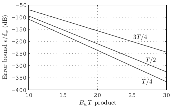
Figure 3: Error bound $\epsilon/\delta_{w}$ using the values for $\delta$ and $\epsilon$ in (40), for $T_{1}=3T/4,T/2,T/4$.

IV Low sensitivity sampling of a sparse trigonometric polynomial

The generic sampling problem for sparse trigonometric polynomials, as posed in Sec. II, Eqs. (19) and (20), does not impose any constraint on the distribution of the instants $t_{n}$. However, the condition number of (20) can vary wildly with it, as can be easily checked numerically. The distribution in which the sampling points are equally spaced and cover $R(0,T)$ is interesting, because it exploits the sparseness of the polynomial, i.e, it produces equations in which most coefficients are zero.

To see this point, assume ${\mathrm{\alpha}}(t;J)$ is uniformly sampled at

$$t_{q+1}\equiv t_{0}+\frac{q}{Q}T,$$ (42)

for $q=0,1,\ldots,Q-1$, $Q>0$, where $t_{0}$ is an arbitrary instant, and define the coefficients

$$\delta_{p}\equiv\beta_{p}{\mathrm{e}}^{j2\pi pt_{0}/T}.$$ (43)

Next, compute the DFT of the sequence ${\mathrm{\alpha}}(t_{q+1};J)$ (divided by $Q$), defining a corresponding set of coefficients $\Lambda_{r}$:

$$\begin{array}[]{l}\displaystyle\Lambda_{r}\equiv\frac{1}{Q}\sum_{q=0}^{Q-1}{\mathrm{\alpha}}(t_{q+1};J){\mathrm{e}}^{-j2\pi rq/Q}\\ \displaystyle=\frac{1}{Q}\sum_{q=0}^{Q-1}\sum_{p\in J}\beta_{p}{\mathrm{e}}^{j2\pi pt_{q+1}/T}{\mathrm{e}}^{-j2\pi rq/Q}\\ \displaystyle=\frac{1}{Q}\sum_{q=0}^{Q-1}\sum_{p\in J}\beta_{p}{\mathrm{e}}^{j2\pi p(t_{0}/T+q/Q)}{\mathrm{e}}^{-j2\pi rq/Q}\\ \displaystyle=\sum_{p\in J}\beta_{p}{\mathrm{e}}^{j2\pi pt_{0}/T}\frac{1}{Q}\sum_{q=0}^{Q-1}{\mathrm{e}}^{j2\pi(p-r)q/Q}\\ \displaystyle=\sum_{\genfrac{}{}{0.0pt}{1}{p\in J}{p\equiv r\;(\mathrm{mod}\;Q)}}\beta_{p}{\mathrm{e}}^{j2\pi pt_{0}/T}=\sum_{\genfrac{}{}{0.0pt}{1}{p\in J}{p\equiv r\;(\mathrm{mod}\;Q)}}\delta_{p}.\end{array}$$ (44)

This derivation shows that $\Lambda_{r}$ can be computed either from the samples ${\mathrm{\alpha}}(t_{q+1};J)$ using its definition,

$$\Lambda_{r}=\frac{1}{Q}\sum_{q=0}^{Q-1}{\mathrm{\alpha}}(t_{q+1};J){\mathrm{e}}^{-j2\pi rq/Q},$$ (45)

or from the coefficients $\delta_{p}$ using

$$\Lambda_{r}=\sum_{\genfrac{}{}{0.0pt}{1}{p\in J}{p\equiv r\;(\mathrm{mod}\;Q)}}\delta_{p}.$$ (46)

So, if the samples ${\mathrm{\alpha}}(t_{q+1};J)$ are known, Eq. (45) allows one to compute the $\Lambda_{r}$ with the best possible conditioning, given that DFT matrices have condition number equal to one. And Eq. (46) shows that $\Lambda_{r}$ is just the sum of some of the coefficients $\delta_{p}$ (those with index $p$ congruent with $r$ modulo $Q$). In some cases, the sum in Eq. (46) may contain a single element, and then one of the coefficients $\delta_{r}$ would be revealed by $\Lambda_{r}$, i.e, $\delta_{p}=\Lambda_{r}$ with $p\equiv r(\mathrm{mod}\;\;Q)$ and $0\leq r<Q$. Usually, however there are several summands, but if the $\Lambda_{r}$ are known, then (46) is in any case a sparse linear system of ones and zeroes.

This argument suggests that a regular grid like (42) is a good choice, in order to obtain a well conditioned linear system. But the selection of $Q$ is problematic. On the one hand, if $Q$ is larger than or equal to the difference between the largest and the smallest element in $J$, then the sum in (46) has a single summand, and the $\Lambda_{r}$ reveal the coefficients $\delta_{p}$ completely. But the over-sampling would be too large in this case. On the other hand, if $Q$ is smaller than that difference, the system in (46) could be under-determined. The solution proposed in the sequel consists in adopting a finite version of the SMRS scheme in [13], in which several integer moduli $Q_{1},Q_{2},\ldots,Q_{K}$ are used instead of a single one.

Let us state first the solution of the interpolation problem for this scheme, and then study its sensitivity. For a fixed set of moduli $Q_{k}$, let $t_{k,q+1}$ denote a finite SMRS scheme with initial instant $t_{0}$,

$$t_{k,q+1}=t_{0}+Tq/Q_{k},\;\;q=0,1,\ldots,Q_{k}-1,$$ (47)

and let $\Lambda_{k,r}$ denote the scaled DFT for modulo $Q_{k}$ as in (44),

$$\Lambda_{k,r}\equiv\frac{1}{Q_{k}}\sum_{q=0}^{Q_{k}-1}{\mathrm{\alpha}}(t_{k,q+1};J){\mathrm{e}}^{-j2\pi rq/Q_{k}}.$$ (48)

Then, Eq. (46) for all moduli $Q_{k}$ can be written as

$$\Lambda_{k,r}=\sum_{\genfrac{}{}{0.0pt}{1}{p\in J}{p\equiv r\;(\mathrm{mod}\;Q_{k})}}\delta_{p},$$ (49)

$k=1,2,\ldots,K$, $q=0,1,\ldots,Q_{k}$. This is a linear system with unknowns $\delta_{p}$. If it has full column rank, then its solution can be written is terms of its pseudo-inverse, denoted $\lambda_{p,k,r}$, i.e,

$$\delta_{p}=\sum_{k=1}^{K}\sum_{r=0}^{Q_{k}-1}\lambda_{p,k,r}\Lambda_{k,r}$$ (50)

Now, Eqs. (43) and (19) allow one to write ${\mathrm{\alpha}}(t;J)$ in terms of the coefficients $\delta_{p}$,

$${\mathrm{\alpha}}(t;J)=\sum_{p\in J}\delta_{p}{\mathrm{e}}^{j2\pi p(t-t_{0})/T}.$$ (51)

Finally, if Eqs. (48) and (50) are substituted into this equation, and the summations are then reordered, the result is

$${\mathrm{\alpha}}(t;J)=\sum_{k=1}^{K}\sum_{q=0}^{Q_{k}-1}{\mathrm{\alpha}}(t_{k,q+1};J){\mathrm{\theta}}_{k,q}(t;J,t_{0}),$$ (52)

where

$$\begin{array}[]{l}\displaystyle{\mathrm{\theta}}_{k,q}(t;J,t_{0})\\ {}\hskip 14.22636pt{}\hfill\displaystyle\equiv\frac{1}{Q_{k}}\sum_{p\in J}\Big{(}\sum_{r=0}^{Q_{k}-1}\lambda_{p,k,r}{\mathrm{e}}^{-j2\pi rq/Q_{k}}\Big{)}{\mathrm{e}}^{j2\pi p(t-t_{0})/T}.\end{array}$$ (53)

The last two equations specify the solution to the interpolation problem using the finite SMRS scheme. Note that (52) can be used to reconstruct any component of ${\mathrm{\alpha}}(t;J)$, simply by restricting the index set in ${\mathrm{\theta}}_{k,q}(t;J,t_{0})$, i.e, if $J^{\prime}\subset J$, then

$${\mathrm{\alpha}}(t;J^{\prime})=\sum_{k=1}^{K}\sum_{q=0}^{Q_{k}-1}{\mathrm{\alpha}}(t_{k,q+1};J){\mathrm{\theta}}_{k,q}(t;J^{\prime},t_{0}).$$ (54)

Also, note that here ${\mathrm{\theta}}_{k,q}(t;J,t_{0})$ is the specific reconstruction function in the SMRS scheme with initial instant $t_{0}$, while ${\mathrm{\theta}}_{n}(t;J)$ in Sec. II, Eq. (22), is a reconstruction function for a generic sampling set $t_{1},t_{2},\ldots,t_{N}$ and fixed $\tau$.

The selection of the moduli $Q_{k}$ can be done now so as to make this method viable, i.e, so that the linear system in (49) has full column rank, and the sensitivity to perturbations of (52) is low. Let us define first the sensitivity measure

$${\mathrm{\gamma}}(t;J^{\prime},t_{0})\equiv(\sum_{k=1}^{K}\sum_{q=0}^{Q_{k}-1}|{\mathrm{\theta}}_{n}(t_{k,q};J^{\prime},t_{0})|^{2})^{1/2}.$$ (55)

and its supremum in $R(0,T)$,

$${\mathrm{\gamma}}(J^{\prime})\equiv\sup_{-T/2\leq t<T/2}{\mathrm{\gamma}}(t;J^{\prime},0).$$ (56)

${\mathrm{\gamma}}(t;J^{\prime},t_{0})$ is the standard deviation factor due to any perturbations in the samples ${\mathrm{\alpha}}(t_{k,q};J^{\prime})$. So, if these samples are contaminated by perturbations of zero mean and variance $\sigma^{2}$, then the value of ${\mathrm{\alpha}}(t;J^{\prime})$ computed using (54) has variance $\sigma^{2}{\mathrm{\gamma}}^{2}(t;J^{\prime},t_{0})$.

The following method gives a suitable collection of moduli $Q_{k}$:

1. Select positive integers $Q_{1}$ and $K$ following $Q_{1}K\approx|J|$ and then set $Q_{k}=Q_{1}+k-1$, $k=2,\ldots,K$.

2. Check whether the linear system

   $$\Lambda_{k,r}=\sum_{\genfrac{}{}{0.0pt}{1}{p\in J}{p\equiv r\;(\mathrm{mod}\;Q_{k})}}\delta_{p}$$ (57)

   is over-determined (or determined). If not increase either $K$ or $Q_{1}$.

3. Finally, the sensitivity can be reduced by adding other $Q$ which are selected so as to minimize ${\mathrm{\gamma}}(J)$, or ${\mathrm{\gamma}}(J^{\prime})$ if the performance for a specific components $J^{\prime}\subset J$ must be improved.

V Interpolation of a bounded multiband signal using the SMRS scheme

As shown in Sec. III, Eq. (37), the sampling problem for a bounded multiband signal ${\mathrm{z}}(t)$ can be reduced to a problem of the same type, but involving a sparse trigonometric polynomial. Specifically, it was shown that there is a polynomial $\tilde{{\mathrm{z}}}(t;\tau)$ such that

$${\mathrm{z}}(\tau+t)\approx\frac{\tilde{{\mathrm{z}}}(t;\tau)}{{\mathrm{w}}(t)},$$ (58)

where $t$ lies in $R(0,T)$. This formula specifies how the multiband signal ${\mathrm{z}}(t)$ can be interpolated if the polynomial $\tilde{{\mathrm{z}}}(t;\tau)$ is known, and how the polynomial $\tilde{{\mathrm{z}}}(t;\tau)$ can be obtained from samples of ${\mathrm{z}}(t)$.

The objective of this section is to show that the finite SMRS scheme in the previous section of the form

$$t_{0}+Tq/Q_{k},\;\;q=0,1,\ldots,Q_{k}-1,\;\;k=1,2,\ldots,K,$$ (59)

can be integrated into the infinite SMRS scheme

$$nT+Tq/Q_{k},\;\;n\;\;\mathrm{in}\;\;\mathbb{Z},\;\;q=0,1,\ldots,Q_{k}-1.$$ (60)

More precisely, there is a $t_{0}$ such that there is a one-to-one correspondence between the samples of ${\mathrm{z}}(t)$ in the scheme (60) that lie in $R(\tau,T)$, and those of $\tilde{{\mathrm{z}}}(t;\tau)$ in the scheme (59). To demonstrate this, assume that it is necessary to sample $\tilde{{\mathrm{z}}}(t;\tau)$ at one of the instants in (59). Let $n_{k,q}(t_{0})$ denote the unique integer such that $t_{0}+Tq/Q_{k}+n_{k,q}(t_{0})T$ lies in $R(0,T)$,

$$n_{k,q}(t_{0})\equiv\lceil(\tau-t_{0})/T-1/2-q/Q_{k}\rceil.$$ (61)

From (58) and recalling that $\tilde{{\mathrm{z}}}(t;\tau)$ is $T$-periodic, it is

$$\begin{array}[]{l}\displaystyle\tilde{{\mathrm{z}}}(t_{0}+Tq/Q_{k};\tau)=\tilde{{\mathrm{z}}}(t_{0}+Tq/Q_{k}+n_{k,q}(t_{0})T;\tau)\\ \displaystyle\approx{\mathrm{z}}(\tau+t_{0}+Tq/Q_{k}+n_{k,q}(t_{0})T)\\ \displaystyle{}\hfill\cdot{\mathrm{w}}(t_{0}+Tq/Q_{k}+n_{k,q}(t_{0})T)\end{array}$$ (62)

The argument of ${\mathrm{z}}$ in this formula belongs to the scheme in (60) for any pair of indices $(k,q)$ if $t_{0}=-\tau$. So, for this $t_{0}$, it is

$$\begin{array}[]{l}\displaystyle\tilde{{\mathrm{z}}}(-\tau+Tq/Q_{k};\tau)\approx{\mathrm{z}}(Tq/Q_{k}+n_{k,q}(-\tau)T){}\\ \displaystyle{}\hfill\cdot{\mathrm{w}}(-\tau+Tq/Q_{k}+n_{k,q}(-\tau)T).\end{array}$$ (63)

This is the one-to-one correspondence between the samples of $\tilde{{\mathrm{z}}}(t;\tau)$ in (59) and those of ${\mathrm{z}}(t)$ in the intersection of (60) with $R(\tau,T)$.

Now, it is possible to write an interpolation formula for ${\mathrm{z}}(t)$. For this it is enough to “sample” $\tilde{{\mathrm{z}}}(t)$ using (63), then obtain the polynomial $\tilde{{\mathrm{z}}}(t)$ approximately using the formula in (54), and finally undoing the windowing [dividing by ${\mathrm{w}}(t)$]. To simplify the notation, define first the instants

$$t^{\prime}_{k,q}(\tau)\equiv-\tau+Tq/Q_{k}+n_{k,q}(-\tau)T.$$ (64)

From (63), the samples of $\tilde{{\mathrm{z}}}(t;\tau)$ are

$$\tilde{{\mathrm{z}}}(-\tau+Tq/Q_{k};\tau)\approx{\mathrm{z}}(\tau+t^{\prime}_{k,q}(\tau)){\mathrm{w}}(t^{\prime}_{k,q}(\tau)).$$ (65)

If the sampling formula in (54) is applied to $\tilde{{\mathrm{z}}}(t;\tau)$ with these sample values, it is

$$\tilde{{\mathrm{z}}}(t;\tau)\approx\sum_{k=1}^{K}\sum_{q=0}^{Q_{k}-1}{\mathrm{z}}(\tau+t^{\prime}_{k,q}(\tau)){\mathrm{w}}(t^{\prime}_{k,q}(\tau)){\mathrm{\theta}}_{k,q}(t;I_{zw},-\tau)$$ (66)

And, finally, (58) gives the desired formula for ${\mathrm{z}}(t)$,

$$\begin{array}[]{l}\displaystyle{\mathrm{z}}(\tau+t)\approx\frac{1}{{\mathrm{w}}(t)}\sum_{k=1}^{K}\sum_{q=0}^{Q_{k}-1}\\ \displaystyle{}\hskip 42.67912pt{\mathrm{z}}(\tau+t^{\prime}_{k,q}(\tau)){\mathrm{w}}(t^{\prime}_{k,q}(\tau)){\mathrm{\theta}}_{k,q}(t;I_{zw},-\tau).\end{array}$$ (67)

The formula for ${\mathrm{s}}_{m}(t)$ is the same but with $I_{zw}$ replaced with $I_{sw,m}$.

VI Error analysis

In the error analysis in the sequel, the sampling scheme is denoted using a single index as $t_{1},t_{2},\ldots,t_{N}$ instead of two, so as to simplify the notation. This also affects the function ${\mathrm{\theta}}_{k,q}(t,J,t_{0})$ in (53), that will be denoted ${\mathrm{\theta}}_{n}(t,J,t_{0})$. Also, the error terms will be written inside square braces for readability.

Let us recall the sampling and interpolation process on ${\mathrm{z}}(t)$ in the last three sections, but keeping track of the different errors, so as to produce an error bound. First, the multiband signal ${\mathrm{z}}(t)$ can be approximated using the polynomial $\tilde{{\mathrm{z}}}_{w}(t;\tau)$, [Eq. (37)],

$${\mathrm{z}}(\tau+t)=\frac{1}{{\mathrm{w}}(t)}\tilde{{\mathrm{z}}}_{w}(t;\tau)+\Big{[}\frac{1}{{\mathrm{w}}(t)}({\mathrm{z}}_{w}(t;\tau)-\tilde{{\mathrm{z}}}_{w}(t;\tau))\Big{]}.$$ (68)

Next, $\tilde{{\mathrm{z}}}_{w}(t;\tau)$ can be reconstructed using the sampling formula in (52) with $t_{0}=-\tau$, $J=I_{zw}$, and samples $\tilde{{\mathrm{z}}}_{w}(t_{n};\tau)$,

$$\tilde{{\mathrm{z}}}_{w}(t;\tau)=\sum_{n=1}^{N}\tilde{{\mathrm{z}}}_{w}(t_{n};\tau){\mathrm{\theta}}_{n}(t;I_{zw},-\tau).$$ (69)

The samples $\tilde{{\mathrm{z}}}_{w}(t_{n};\tau)$ are approximately equal to ${\mathrm{z}}(\tau+t_{n}){\mathrm{w}}(t_{n})$:

$$\tilde{{\mathrm{z}}}_{w}(t_{n};\tau)={\mathrm{z}}(\tau+t_{n}){\mathrm{w}}(t_{n})+\Big{[}\tilde{{\mathrm{z}}}_{w}(t_{n};\tau)-{\mathrm{z}}_{w}(t_{n};\tau)\Big{]}.$$ (70)

But ${\mathrm{z}}(\tau+t_{n})$ may be contaminated by a perturbation, denoted ${\mathrm{\eta}}(t_{n})$:

$${\mathrm{z}}(\tau+t_{n})={\mathrm{z}}(\tau+t_{n})+{\mathrm{\eta}}(t_{n})+\Big{[}-{\mathrm{\eta}}(t_{n})\Big{]}.$$ (71)

Next, replace in (70) the term ${\mathrm{z}}(\tau+t_{n})$ with the right side of (71), so as to obtain

$$\begin{array}[]{l}\displaystyle\tilde{{\mathrm{z}}}_{w}(t_{n};\tau)=({\mathrm{z}}(\tau+t_{n})+{\mathrm{\eta}}(t_{n})){\mathrm{w}}(t_{n})\\ \displaystyle{}\hskip 28.45274pt+\Big{[}-{\mathrm{\eta}}(t_{n}){\mathrm{w}}(t_{n})+\tilde{{\mathrm{z}}}_{w}(t_{n};\tau)-{\mathrm{z}}_{w}(t_{n};\tau)\Big{]}.\end{array}$$ (72)

In turn, substitute this equation into (69), and finally use the result to replace the term $\tilde{{\mathrm{z}}}_{w}(t;\tau)$ in (68). The outcome of these replacements is a formula with error term for ${\mathrm{z}}(\tau+t)$:

$$\begin{array}[]{l}\displaystyle{\mathrm{z}}(\tau+t)=\frac{1}{{\mathrm{w}}(t)}\sum_{n=1}^{N}({\mathrm{z}}(\tau+t_{n})+{\mathrm{\eta}}(t_{n})){\mathrm{w}}(t_{n}){\mathrm{\theta}}_{n}(t;I_{zw},-\tau)\\ \displaystyle+\Bigg{[}\frac{1}{{\mathrm{w}}(t)}\sum_{n=1}^{N}(-{\mathrm{\eta}}(t_{n}){\mathrm{w}}(t_{n})){\mathrm{\theta}}_{n}(t;I_{zw},-\tau)\\ \displaystyle+\frac{1}{{\mathrm{w}}(t)}\sum_{n=1}^{N}(\tilde{{\mathrm{z}}}_{w}(t_{n};\tau)-{\mathrm{z}}_{w}(t_{n};\tau)){\mathrm{\theta}}_{n}(t;I_{zw},-\tau)\\ \displaystyle+\frac{1}{{\mathrm{w}}(t)}({\mathrm{z}}_{w}(t;\tau)-\tilde{{\mathrm{z}}}_{w}(t;\tau))\Bigg{]}.\\ \end{array}$$ (73)

Now, since ${\mathrm{w}}(t)\leq 1$ in $R(0,T_{1})$, the three error terms can be bounded in the following way. For the first term in (73):

$$\begin{array}[]{l}\displaystyle\Big{|}\frac{1}{{\mathrm{w}}(t)}\sum_{n=1}^{N}(-{\mathrm{\eta}}(t_{n}){\mathrm{w}}(t_{n})){\mathrm{\theta}}_{n}(t;I_{zw},-\tau)\Big{|}{}\\ \displaystyle{}\hfill\leq\frac{A_{\eta}}{{\mathrm{w}}(t)}{\mathrm{\gamma}}(t;I_{z,w},-\tau),\end{array}$$ (74)

where

$$A_{\eta}\equiv\Big{(}\sum_{n=1}^{N}|{\mathrm{\eta}}(t_{n})|^{2}\Big{)}^{1/2}$$ (75)

and

$${\mathrm{\gamma}}(t;I_{z,w},t_{0})\equiv\Big{(}\sum_{n=1}^{N}|{\mathrm{\theta}}_{n}(t;I_{zw},t_{0})|^{2}\Big{)}^{1/2}.$$ (76)

For the second,

$$\begin{array}[]{l}\displaystyle\Big{|}\frac{1}{{\mathrm{w}}(t)}\sum_{n=1}^{N}(\tilde{{\mathrm{z}}}_{w}(t_{n};\tau)-{\mathrm{z}}_{w}(t_{n};\tau)){\mathrm{\theta}}_{n}(t;I_{zw},-\tau)\Big{|}\\ \displaystyle{}\hfill\leq\frac{\epsilon\sqrt{N}}{{\mathrm{w}}(t)}\Big{(}\sum_{m=1}^{M}A_{s,m}\Big{)}{\mathrm{\gamma}}(t;I_{z,w},-\tau).\end{array}$$ (77)

And for the third,

$$\Big{|}\frac{1}{{\mathrm{w}}(t)}({\mathrm{z}}_{w}(t;\tau)-\tilde{{\mathrm{z}}}_{w}(t;\tau))\Big{|}\leq\frac{\epsilon}{{\mathrm{w}}(t)}\sum_{m=1}^{M}A_{s,m}.$$ (78)

So, the final bound is

$$\begin{array}[]{l}\displaystyle\Big{|}{\mathrm{z}}(\tau+t)\\ \displaystyle{}\hfill-\frac{1}{{\mathrm{w}}(t)}\sum_{n=1}^{N}({\mathrm{z}}(\tau+t_{n})+{\mathrm{\eta}}(t_{n})){\mathrm{w}}(t_{n}){\mathrm{\theta}}_{n}(t;I_{zw},-\tau)\Big{|}\\ \displaystyle\leq\frac{A_{\eta}{\mathrm{\gamma}}(t;I_{z,w},-\tau)}{{\mathrm{w}}(t)}\\ \displaystyle{}\hfill+\frac{\epsilon}{{\mathrm{w}}(t)}\Big{(}\sum_{m=1}^{M}A_{s,m}\Big{)}\Big{(}\sqrt{N}{\mathrm{\gamma}}(t;I_{z,w},-\tau)+1\Big{)}.\\ \end{array}$$ (79)

The first term is due to the sensitivity of the linear system. The second is due to the mismatch and perturbations, and it can be arbitrarily small, since $\epsilon$ tends to zero exponentially with $T$, [Eq. (40)].

The error analysis can be repeated for the components ${\mathrm{s}}_{m}(t)$, following the same method, and the result is

$$\begin{array}[]{l}\displaystyle\Big{|}{\mathrm{s}}_{m}(\tau+t)\\ \displaystyle{}\hfill-\frac{1}{{\mathrm{w}}(t)}\sum_{n=1}^{N}({\mathrm{z}}(\tau+t_{n})+{\mathrm{\eta}}(t_{n})){\mathrm{w}}(t_{n}){\mathrm{\theta}}_{n}(t;I_{sw,m},-\tau)\Big{|}\\ \displaystyle\leq\frac{A_{\eta}{\mathrm{\gamma}}(t;I_{sw,m})}{{\mathrm{w}}(t)}\\ \displaystyle{}\hfill+\frac{\epsilon}{{\mathrm{w}}(t)}\Big{(}\Big{(}\sum_{m=1}^{M}A_{s,m}\Big{)}\sqrt{N}{\mathrm{\gamma}}(t;I_{sw,m},-\tau)+A_{s,m}\Big{)}.\\ \end{array}$$ (80)

VII Blind estimation of the spectral support

If the spectral support of the multiband signal is unknown, then it is not possible to determine the set $I_{zw}$, and thus the procedure presented in the previous sections is not applicable in principle. In the literature [8, 13], this problem has been addressed using compressed sensing techniques. For the SMRS scheme in Secs. IV and V, this approach would lead to a linear system like that in (57), but in which the $l^{1}$ norm of the set of coefficients $d_{p}$ must be minimized

$$\{\delta_{p}\}=\arg\min\sum_{p=P_{1}}^{P_{2}}|\delta_{p}|\;\;\mathrm{subject\;to}\;\;\Lambda_{k,r}=\sum_{p=P_{1}}^{P_{2}}\delta_{p}.$$ (81)

Here, $\{\delta_{p}\}$ denotes the set of coefficients $\delta_{p}$, and the frequency indices are assumed to lie in $[P_{1},P_{2}]$. However, the multiband signal ${\mathrm{z}}(t)$ can be approximated in several intervals $R(\tau_{h},T)$, $h=1,2,\ldots,H$, with distinct $\tau_{h}$ using polynomials $\tilde{{\mathrm{z}}}_{w}(t;\tau_{h})$. These polynomials have the same index support $I_{zw}$ and, besides, the $\tau_{h}$ can be selected in the infinite SMRS scheme, so that the relative sampling instants $t_{k,q}$ are the same for all of them. In this setting, the blind estimation problem can be viewed as a compressed sensing problem with multiple measurements vectors (MMV), [24]. Nevertheless, since the duration of the multiband signal can be arbitrarily large, the blind problem can be posed using any of the techniques from direction of arrival (DOA) estimation, [25, chapters 8 and 9]. This alternative solution is analyzed in the next sub-section, where the MUSIC algorithm is adopted. It is then tested numerically in Sec. VIII-C.

A final aspect is whether the SMRS scheme leads to a full column rank linear system, for any set $I_{zw}$. In the literature, a sampling scheme of this kind is termed “universal”, [8, 13]. It turns out that the finite SMRS scheme in Sec. IV can be converted into a universal one in a simple way. To see this, recall the explicit expression for $\tilde{{\mathrm{z}}}_{w}(t;\tau)$ in (35),

$${\mathrm{z}}_{w}(t;\tau)\approx\tilde{{\mathrm{z}}}_{w}(t;\tau)=\sum_{p\in I_{zw}}{\mathrm{c}}_{p}(\tau){\mathrm{e}}^{j2\pi pt/T},$$ (82)

and assume that the sampling scheme is multi-coset sampling with repetition period $T$ and minimum spacing $\Delta t$. This means that $\tilde{{\mathrm{z}}}_{w}(t;\tau)$ is sampled at instants $t_{0}+n_{r}\Delta t$, $r=1,2,\ldots,R$, where the $n_{r}$ are distinct integers, $R\Delta t=T$, and $R\geq|I_{zw}|$. Evaluating (82) at the sampling instants yields

$$\tilde{{\mathrm{z}}}_{w}(t_{0}+n_{r}\Delta t;\tau)=\sum_{p\in I_{zw}}{\mathrm{c}}_{p}(\tau){\mathrm{e}}^{j2\pi pt_{0}/T}{\mathrm{e}}^{j2\pi pn_{r}/R}.$$ (83)

This linear system may not have full column rank. However, note that (82) is also valid if $T$ is replaced with a $T^{\prime}$ following $T^{\prime}>T$, given the $L^{1}$ norm of ${\mathrm{z}}_{w}(t;\tau)$ in $R(0,T^{\prime})$ is larger than in $R(0,T)$, and the interpolation accuracy was already enough in $R(0,T)$. To replace $T$ with $T^{\prime}$ may slightly increase the number of elements of $|I_{zw}|$, i.e, the spectral sampling will be finer, and in general there will be two different sets $I_{zw}(T)$ and $I_{zw}(T^{\prime})$. However, if the difference $R-|I_{zw}(T)|\geq 0$ is large enough, then one may expect that it is also $R-|I_{zw}(T^{\prime})|\geq 0$, i.e, the linear system for the larger period $T^{\prime}$ will also have more equations than unknowns. Knowing this, take $T^{\prime}=\Delta tP$ where $P$ is the smallest prime number following $P\geq R$, and evaluate (82) with $T^{\prime}$ in place of $T$,

$${\mathrm{z}}_{w}(t_{0}+n_{r}\Delta t;\tau)\approx\sum_{p\in I_{zw}}{\mathrm{c}}_{p}(\tau){\mathrm{e}}^{j2\pi pt_{0}/T^{\prime}}{\mathrm{e}}^{j2\pi pn_{r}/P}.$$ (84)

If $R-|I_{zw}(T^{\prime})|\geq 0$ this system has full column rank, since all minors of trigonometric Vandermonde matrices of prime order have full rank, by Chebotarev’s theorem; (see [26, page 25]). So, for ${\mathrm{z}}_{w}(t;\tau)$ one can turn a multi-coset sampling scheme into a universal one by slightly increasing $T$. The only condition for this is that there must be a minimum over-sampling, in the sense that the difference $R-|I_{zw}(T^{\prime})|$ must not be too small.

Finally, note that the SMRS scheme in Sec. IV is a multi-coset scheme if one sets $t_{0}=-\tau$ and

$$\Delta t=T/(\nu\,\mathrm{lcm}_{k}Q_{k}),$$ (85)

where $\mathrm{lcm}$ denotes the least common multiple and $\nu$ is any positive integer. So, the method of perturbing $T$ also works for SMRS sampling. In practice, the difference between using $T$ or $T^{\prime}$ can be immaterial. For example, in Sec. VIII-B, the SMR scheme uses the $Q$ values in (101) with

$$\prod_{k=1}^{K}Q_{k}=159049016335440.$$ (86)

This product is one of the possible denominators in (85) for a specific $\nu$, and the smallest prime $P$ following $P\geq\prod_{k=1}^{K}Q_{k}$ is

$$P=159049016335453.$$ (87)

So, the relative perturbation of $T$ is

$$\frac{T^{\prime}-T}{T}=\frac{P}{R}-1=8.17\cdot 10^{-14},$$ (88)

which is well below the numerical precision in that section.

VII-A Blind sampling of a collection of sparse trigonometric polynomials with common index support

Consider a collection of trigonometric polynomials ${\mathrm{\alpha}}_{1}(t;J),{\mathrm{\alpha}}_{2}(t;J),\ldots,{\mathrm{\alpha}}_{H}(t;J)$ with common index support $J$ and coefficients $\beta_{h,p}$ of the form in (19),

$${\mathrm{\alpha}}_{h}(t;J)\equiv\sum_{p\in J}\beta_{h,p}{\mathrm{e}}^{j2\pi pt/T}.$$ (89)

Assume that each polynomial is sampled at the distinct epochs $t_{1},t_{2},\ldots,t_{N}$. If the samples are denoted by $\hat{\alpha}_{h,n}$,

$$\hat{\alpha}_{h,n}=\alpha_{h}(t_{n};J)+\mu_{h,n},$$ (90)

where $\mu_{h,n}$ is an unknown perturbation, then Eq. (89) yields the following model for $\hat{\alpha}_{h,n}$,

$$\hat{\alpha}_{h,n}=\sum_{r=1}^{|J|}\beta_{h,p(r)}{\mathrm{e}}^{j2\pi p(r)t_{n}/T}+\mu_{h,n},$$ (91)

where $p(r)$ is an ordering of $J$, i.e, $p(r)$ runs through all elements of $J$ for $r=1,2,\ldots,|J|$. Next, it is straight-forward to convert this equation into a matrix model, similar to those in DOA estimation. For this, define the matrices

$$\begin{array}[]{l@{\;}l@{\;}l}[\mbox{\boldmath$\mathbf{A}$\unboldmath}]_{n,h}\equiv\hat{\alpha}_{h,n},&[\mbox{\boldmath$\mathbf{B}$\unboldmath}]_{r,h}\equiv\beta_{h,p(r)},&[\mbox{\boldmath$\mathbf{N}$\unboldmath}]_{n,h}\equiv\mu_{h,n},\\ {[}\mbox{\boldmath$\mathbf{p}$\unboldmath}]_{r}\equiv p(r),&[\mbox{\boldmath$\mathbf{\phi}$\unboldmath}(p)]_{n}\equiv{\mathrm{e}}^{j2\pi pt_{n}/T},&[\mbox{\boldmath$\mathbf{\Phi}$\unboldmath}(\mbox{\boldmath$\mathbf{p}$\unboldmath})]_{\cdot,r}\equiv\mbox{\boldmath$\mathbf{\phi}$\unboldmath}([\mbox{\boldmath$\mathbf{p}$\unboldmath}]_{r}).\end{array}$$ (92)

The model is

$$\mbox{\boldmath$\mathbf{A}$\unboldmath}=\mbox{\boldmath$\mathbf{\Phi}$\unboldmath}(\mbox{\boldmath$\mathbf{p}$\unboldmath})\mbox{\boldmath$\mathbf{B}$\unboldmath}+\mbox{\boldmath$\mathbf{N}$\unboldmath}.$$ (93)

The purpose now is to estimate the elements of $\mathbf{p}$, which specify the spectral support of the polynomials $\tilde{{\mathrm{z}}}_{w}(t;\tau_{h})$, and the matrix of coefficients $\mathbf{B}$. In principle, it is possible to apply to (93) a wide variety of algorithms for DOA estimation in array processing, [25, Chapters 8 and 9]. However, this estimation/detection problem has a few differences relative to the typical DOA problems: the length of $\mathbf{p}$ can be large (on the hundreds), the components of this vector must be integers and, as will be shown in the numerical examples, the problem of detecting the number of components of $\mathbf{p}$ is not critical.

An algorithm that seems well suited for (93) is MUSIC, [27]. If $P$ denotes an upper bound for $|I_{zw}|$, and $\mathbf{U}$ is an $N\times(N-P)$ matrix that spans the noise subspace of $\mathbf{A}$, $\mbox{\boldmath$\mathbf{U}$\unboldmath}^{\mathrm{H}}\mbox{\boldmath$\mathbf{U}$\unboldmath}=\mbox{\boldmath$\mathbf{I}$\unboldmath}$, then the normalized MUSIC spectrum is

$${\mathrm{\chi}}(p)\equiv\frac{||\mbox{\boldmath$\mathbf{\phi}$\unboldmath}(p)||^{2}}{||\mbox{\boldmath$\mathbf{U}$\unboldmath}^{\mathrm{H}}\mbox{\boldmath$\mathbf{\phi}$\unboldmath}(p)||^{2}}.$$ (94)

The effectiveness of this estimator will be demonstrated in the numerical example in Sec. VIII-C.

VIII Numerical examples

VIII-A Validation of the interpolation method

In Secs. II and III, a basic argument was that a band-limited signal which is concentrated in a time interval can be well approximated by a trigonometric polynomial, and this concentration was achieved by means of a window function. To test this property numerically, a BPSK signal ${\mathrm{s}}(t)$ was generated, whose modulating pulse was a raised cosine with roll-off factor 0.8, peak amplitude $A_{s}=1$, and bandwidth $B=136/T$, (chip period $T_{c}=0.01324T$). The formula for this signal is

$$\sum_{p=-\infty}^{\infty}a_{p}{\mathrm{g}}_{rc}(t-pT_{c}),$$ (95)

where ${\mathrm{g}}_{rc}(t)$ is the raised-cosine pulse

$${\mathrm{g}}_{rc}(t)\equiv\pi\,\mathrm{{\mathrm{sinc}}}\Big{(}\frac{t}{T_{c}}\Big{)}\frac{\cos(\pi\beta t/T_{c})}{1-(2\beta t/T_{c})^{2}},$$ (96)

and the coefficients $a_{p}$ took two real values $\pm A^{\prime}$ at random. $A^{\prime}$ was selected so that the peak amplitude of the signal is $A_{s}$. Then, the window in Sec. III-A was applied to this signal with $B_{w}=13.6/T$ and $\delta=0.0103$ at $\tau=0$. This gives $\epsilon=10^{-8}$. Fig. 1 shows the BPSK signal, the window ${\mathrm{w}}(t)$, and the windowed signal (bold line). The BPSK signal can be regarded as a multiband signal with a single component and spectral support $[-B/2,B/2]$. Therefore, the results in Sec. III apply, and there is a set of coefficients ${\mathrm{c}}_{p}(0)$ such that

$${\mathrm{s}}(t)\approx\frac{1}{{\mathrm{w}}(t)}\sum_{p=-p_{B}}^{p_{B}}{\mathrm{c}}_{p}(0){\mathrm{e}}^{j2\pi pt/T}$$ (97)

where $p_{B}\equiv\lfloor(B+B_{w})T/2\rfloor$. In order to check whether this is an accurate model, the signal ${\mathrm{s}}(t){\mathrm{w}}(t)$ was sampled with rate $1/(4(B+B_{w}))$ (over-sampling factor 4), and then a polynomial like that on the right of (97) was fitted to these data using least squares. Then, the resulting polynomial, but divided by ${\mathrm{w}}(t)$, was used to approximate the initial BPSK signal. Fig. 2 presents the error of this procedure. Note that it increases toward the interval limits due to ${\mathrm{w}}(t)$, but the interpolation error is very small. Actually, for $t$ in roughly $R(0,T/2)$, it is below -200 dB.

VIII-B Performance in the presence of noise

In order to test the performance in the presence of noise, a multiband signal with five components was generated. Its components were signals of one of the following types:

1. QPSK signal modulated by a raised cosine pulse with roll-off factor 0.8. This signal has the form in Eq. (95), but with symbols in the constellation $\pm A^{\prime}\pm jA^{\prime}$. $A^{\prime}$ was selected so that the peak absolute value of the signal was one.

2. Sum of 150 undamped exponentials with random phases and frequencies,

   $$\sum_{p=1}^{150}a_{p}{\mathrm{e}}^{j(2\pi f_{p}t+\phi_{p})}.$$ (98)

   The phases were taken at random in the interval $[0,2\pi]$, and the amplitudes $a_{p}$ in the interval $[0,1]$. These amplitudes were then scaled so that the peak amplitude of the signal was equal to one. The frequencies were taken at random in the interval $[-B/2,B/2]$, where $B$ is the bandwidth assigned to the signal.

3. Sum of 200 delayed sinc pulses with random delays and amplitudes

   $$\sum_{p=1}^{200}a_{p}\mathrm{sinc}(B(t-\tau_{p})).$$ (99)

   The delays were taken at random in $R(0,2T)$, knowing that the sampling interval is $R(0,T)$. The amplitudes $a_{p}$ had random absolute value in $[0,1]$ and random phase in $[0,2\pi]$. They were then scaled so that the peak amplitude of the signal was one.

In this example the time and frequency variables were normalized so that $T=1$. For the five components, the component index ($m$), type of signal (type), central frequency ($f_{c}$), bandwidth ($B$), bandwidth after windowing ($B^{\prime}$), and the first ($f_{a}$) and last ($f_{b}$) frequencies in the trigonometric approximation were the following:

$m$	type	$f_{c}$	$B$	$B^{\prime}$	$f_{a}$	$f_{b}$
1	1	308.892	60.4428	69.5628	275	343
2	2	596.276	41.7585	50.8785	571	621
3	3	920.824	39.9765	49.0965	897	945
4	1	1169.11	66.6665	75.7865	1132	1207
5	2	1381.22	19.1557	28.2757	1368	1395

These bands are schematically plotted in Fig. 4.

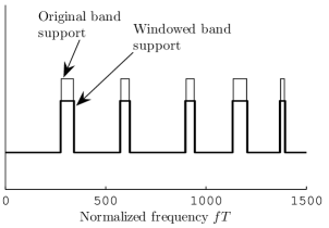
Figure 4: Supports of the multiband signal before and after windowing in Sec. VIII-B. The amplitude along the $y$-axis has no meaning. For the numerical values that specify these bands, see table in Sec. VIII-B.

A set of moduli $Q$ was selected using the method in Sec. IV, [around Eq. (57)]. The set was

$$Q_{k}=67+k,\;k=1,\ldots,\;K,\;\>\>\mbox{with}\>\>K=4.$$ (100)

This set ensured that the linear system in (57) had full column rank and was minimally over-determined. Actually, the number of samples was above the number of unknown coefficients just by one; (274 samples were taken, but there were 273 unknowns). However, the noise factor in (56) was ${\mathrm{\gamma}}(I_{zw})=48.75$ dB, that is, there were interpolation instants in which the signal-to-noise ratio would be degraded 48.75 dB, (assuming complex white noise). In order to reduce this figure, several sampling grids were added. The final set of $Q$ values was

$$11,18,19,37,49,68,69,70,71.$$ (101)

These additional $Q$ values were selected so as to reduce ${\mathrm{\gamma}}(I_{zw})$ as much as possible sequentially. With the set in (101), the noise figure was ${\mathrm{\gamma}}(I_{zw})=18.77$ dB, i.e, in the worst case the noise would be amplified 18.77 dB. Fig. 5 shows ${\mathrm{\gamma}}(t,I_{zw})$.

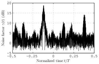
Figure 5: Noise factor in example of Sec. VIII-B.

Note that except for a few peaks, ${\mathrm{\gamma}}(t,I_{zw})$ is well below this figure. The performance in terms of bandwidths and rates was the following:

Nyquist bandwidth:	1112.13
Landau limit:	228
Landau limit after windowing:	273.6
Sampling rate:	394
(Nyquist rate)/(Sampling rate):	2.82
(Sampling rate)/(Landau limit):	1.73

The sampling rate equaled 394, that is, it was only necessary to take this number of samples in each period $T$. The ratio between the sampling rate and the Landau limit shows how far this implementation was from the minimal sampling rate (factor 1.73). This extra over-sampling was produced by the windowing and by the over-determination of the linear system so as to reduce ${\mathrm{\gamma}}(I_{zw})$. Relative to the usual Nyquist rate, this implementation afforded a sampling rate reduction of factor 2.82.

As commented in Sec. IV, the linear system that must be solved for obtaining the coefficients $\delta_{p}$ is that in (57), which is a sparse system. In this example, the matrix corresponding to (57) has only 2.18% of non-zero elements which are equal to one. Thus, solving this system using an efficient method for sparse linear systems, like that in [28], could be more efficient than directly multiplying by the pseudo-inverse of the matrix corresponding to (57).

Fig. 6 shows the module of the coefficients $\delta_{p}$ in this example, assuming that the ratio between the power of the multiband signal and the noise was 70 dB. The noise component in these coefficients is also plotted in this figure. Note that the coefficients $\delta_{p}$ are correctly estimated with signal-to-noise ratio equal to 54.6 dB.

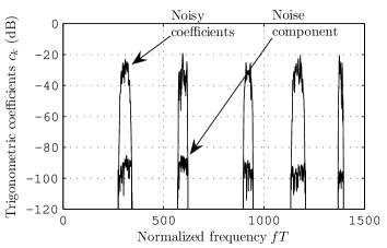
Figure 6: Noisy trigonometric coefficients $c_{k}$ and their noise component in Sec. VIII-B.

Finally, Fig. 7 shows the error in the interpolation of the first multiband component, together with the error bound in (80). Note that the error is small in a wide range and that the bound is very conservative.

Figure 7: Interpolation error for the first multiband component in example in Sec VIII-B, and corresponding error bound in (80).

VIII-C Blind sampling

In order to test the MUSIC algorithm in Sec. VII-A, the example in the previous section was repeated but for QPSK signals (in order to reduce the computational load). Also, the set of moduli $Q_{k}$ was changed to

$$20,50,70,110,130,$$ (102)

so that all moduli $Q_{k}$ have common factor 10. Due to this property, the sampling scheme had period $T/10$, which made it possible to use the central instants $\tau_{h}=Th/10$, i.e, the multiband signal was windowed in $H=500$ consecutive intervals $R(Th/10,T)$ with 90% overlap. Fig. 8(a) shows the MUSIC spectrum in Eq. (94) assuming a signal subspace of dimension $P=|I_{zw}|$. Note that this estimator is able to detect the multiband components as well as their approximate width. (Compare this figure with Fig. 4.) Figs. 8(b) and 8(c) show the same spectrum but assuming a signal subspace of dimension $|I_{zw}|-50$ and $|I_{zw}|+50$, respectively. Note that the detection capability remains unchanged, relative to the case $P=|I_{zw}|$ in Fig. 8(a).

(a) $P=|I_{zw}|$

(b) $P=|I_{zw}|-50$.

(c) $P=|I_{zw}|+50$

Figure 8: MUSIC spectra in Sec. VIII-C.

IX Conclusions

A method for sampling bounded multiband signals has been presented, that makes it possible to approach the Landau limit, while keeping at the same time the noise sensitivity at a low level. The method is based on approximating the product of the signal with a window function by means of a trigonometric polynomial. This polynomial “inherits” the multiband property from the signal. The associated sampling scheme is the recently proposed synchronous multi-rate sampling. Also, it was shown that the blind sampling of a bounded multiband signal can be reduced to the sampling of a collection of multiband trigonometric polynomials with unknown index support. This fact made it possible to apply a DOA estimation algorithm (MUSIC) for the detection of the spectral support. The performance of the methods in the paper have been validated in several numerical examples.

X Acknowledgments

The author would like to thank the editor and reviewers of this paper for their thorough revision and the many useful comments.

Appendix A Bound on the tails of the window function

The computation of the error bound $\epsilon$ in Eq. (18) depends on bounding the series

$${\mathrm{S}}(a,b)\equiv\sum_{n=0}^{\infty}\frac{1}{(a+n)\sqrt{(a+n)^{2}-b^{2}}}$$ (103)

for constants $a>b>0$. For this, introduce first the variable change

$$x(n)=\Big{(}\frac{b}{a+n}\Big{)}^{2}$$ (104)

to obtain

$$\begin{array}[]{r@{\,=\,}l}\displaystyle{\mathrm{S}}(a,b)&\displaystyle\sum_{n=0}^{\infty}\frac{1}{(a+n)^{2}}\frac{1}{\sqrt{1-(b/(a+n))^{2}}}\\ &\displaystyle\frac{1}{b^{2}}\sum_{n=0}^{\infty}\frac{x(n)}{\sqrt{1-x(n)}}.\end{array}$$ (105)

The function $1/\sqrt{1-x}$ is increasing in $[0,1[$ and the maximum value of $x=x(n)$ in (104) is $(b/a)^{2}$. So, this function can be bounded as

$$\frac{1}{\sqrt{1-x(n)}}\leq\frac{1}{\sqrt{1-(b/a)^{2}}}=\frac{a}{\sqrt{a^{2}-b^{2}}}.$$ (106)

Coming back to (105), it follows that

$$\begin{array}[]{r@{\,}c@{\,}l}\displaystyle{\mathrm{S}}(a,b)&\displaystyle\leq&\displaystyle\frac{a}{b^{2}\sqrt{a^{2}-b^{2}}}\sum_{n=0}^{\infty}x(n)=\frac{a}{\sqrt{a^{2}-b^{2}}}\sum_{n=0}^{\infty}\frac{1}{(a+n)^{2}}\\ &\displaystyle=&\displaystyle\frac{1}{\sqrt{1-(b/a)^{2}}}{\mathrm{\psi}}^{\prime}(a),\\ \end{array}$$ (107)

where ${\mathrm{\psi}}^{\prime}(a)$ is the derivative of the polygamma function.

Let us proceed with the derivation of the bound. Recalling the definitions in Eqs. (38) and (39), since the sine function is bounded by one, it is

$$\begin{array}[]{l}\displaystyle|{\mathrm{w}}(t)|\leq\frac{1}{\pi\delta B_{w}t}\frac{1}{\pi(1-\delta)B_{w}\sqrt{t^{2}-\rho^{2}T^{2}/4}}{}\\ \displaystyle{}\hfill\cdot\frac{1}{\mathrm{sinc}(j(1-\delta)\rho B_{w}T/2)}\\ \displaystyle=\frac{1}{\mathrm{sinc}(j(1-\delta)\rho B_{w}T/2)\pi^{2}\delta(1-\delta)B_{w}^{2}t\sqrt{t^{2}-\rho^{2}T^{2}/4}}\\ \displaystyle=C\frac{1}{t\sqrt{t^{2}-\rho^{2}T^{2}/4}},\end{array}$$ (108)

where $C$ is the constant

$$C\equiv\big{(}\mathrm{sinc}(j(1-\delta)\rho B_{w}T/2)\pi^{2}\delta(1-\delta)B_{w}^{2}\big{)}^{-1}.$$ (109)

Now,

$$\begin{array}[]{l}\displaystyle\sum_{p=2}^{\infty}|{\mathrm{w}}(t+pT)|\leq C\sum_{p=2}^{\infty}\frac{1}{(t+pT)\sqrt{(t+pT)^{2}-\rho^{2}T^{2}/4}}\\ \displaystyle=\frac{C}{T^{2}}\sum_{p=2}^{\infty}\frac{1}{(t/T+p)\sqrt{(t/T+p)^{2}-\rho^{2}/4}}\\ \displaystyle=\frac{C}{T^{2}}{\mathrm{S}}(2+t/T,\rho/2).\end{array}$$ (110)

Also,

$$\begin{array}[]{l}\displaystyle\sum_{p=2}^{\infty}|{\mathrm{w}}(t-pT)|=\sum_{p=2}^{\infty}|{\mathrm{w}}(-t+pT)|\leq\frac{C}{T^{2}}{\mathrm{S}}(2-t/T,\rho/2).\end{array}$$ (111)

So, combining the last two inequalities, it is

$$\begin{array}[]{l}\displaystyle\sum_{|p|>1}|{\mathrm{w}}(t+pT)|{}\\ \displaystyle{}\hfill\leq\frac{C}{T^{2}}({\mathrm{S}}(2-t/T,\rho/2)+{\mathrm{S}}(2+t/T,\rho/2)),\end{array}$$ (112)

and

$$\begin{array}[]{l}\displaystyle\sum_{p\neq 0}|{\mathrm{w}}(t+pT)|\leq|{\mathrm{w}}(t-T)|+|{\mathrm{w}}(t+T)|\\ \displaystyle\hfill+\frac{C}{T^{2}}({\mathrm{S}}(2-t/T,\rho/2)+{\mathrm{S}}(2+t/T,\rho/2)),\end{array}$$ (113)

The final bound is obtained by substituting (107) and (109) into this inequality.

$\tilde{\;}$	Periodic repetition with period $T$, Eq. (5)
$|\cdot|$	$|J|$ is the number of elements of the finite set $J$
$\mathbf{A}$	Data matrix in (92)
$[a_{m},b_{m}]$	Spectral support of ${\mathrm{s}}_{m}(t)$
$A_{\eta}$	$l^{2}$ norm of set of samples ${\mathrm{\eta}}(t_{n})$ in (75)
$A_{s}$	Amplitude of ${\mathrm{s}}(t)$, $|{\mathrm{s}}(t)|\leq A_{s}$
$A_{s,m}$	Amplitude of ${\mathrm{s}}_{m}(t)$
$\hat{\alpha}_{h,n}$	Data value in (90)
${\mathrm{\alpha}}(t_{n};J)$	Generic sparse trigonometric polynomial in (20)
${\mathrm{\alpha}}(t_{n};J)$	Trigonometric polynomial in Eq. (89)
$B$	Two-sided bandwidth of ${\mathrm{s}}(t)$
$B_{w}$	Two-sided bandwidth of ${\mathrm{w}}(t)$, Sec. II
$\mathcal{B}_{\pi B}^{\infty}$	Bernstein space of type $\pi B$
$\beta_{p}$	Coefficient of ${\mathrm{\alpha}}(t;J)$ in (20)
$\beta_{h,p}$	Coefficient of ${\mathrm{\alpha}}_{h}(t;J)$ in (89)
$\mathbf{B}$	Coefficient matrix in (92)
${\mathrm{c}}_{p}(\tau)$	Coefficient of $\tilde{{\mathrm{z}}}_{w}(t;\tau)$
$\delta$	Window parameter in Eq. (38)
$\delta_{p}$	Unknowns in sparse linear system, Eq. (43)
$\delta_{w}$	Lower bound on ${\mathrm{w}}(t)$ in $R(0,T_{1})$, $\delta_{w}>0$, Eq. (41)
$\eta_{p,n}$	Pseudo-inverse of the linear system in (21)
$\mbox{\boldmath$\mathbf{\phi}$\unboldmath}(p)$	Vector of exponentials in (92)
$\mathbf{\Phi}$	Matrix of exponentials in (92)
${\mathrm{\gamma}}(J^{\prime})$	Supremum of sensitivity measure in $R(0,T)$, Eq. (56)
${\mathrm{\gamma}}(t,J^{\prime},t_{0})$	Sensitivity measure in Eq. (55) or (76)
${\mathrm{h}}_{m,n}(t)$	Generic interpolation functions in (9)
$I_{sw,m}$	Index set of polynomial $\tilde{{\mathrm{s}}}_{w,m}(t;\tau)$, Eq. (14)
$I_{zw}$	Index set of polynomial $\tilde{{\mathrm{z}}}_{w}(t;\tau)$, Eq. (15)
$\mathbf{I}$	Identity matrix in Sec. VII-A
$J$, $J^{\prime}$	Arbitrary finite sets of integers (indices)
$\lambda_{p,k,r}$	Pseudo-inverse of linear system in (49)
$M$	Number of multiband components
$\mathbf{N}$	Noise matrix in (92)
$n_{k,q}(t_{0})$	Integer shift in Eq. (61)
$p(r)$	Ordering of set $J$ in (91)
$\mathbf{p}$	Vector of indices in (92)
$R(\tau,T)$	Time interval defined in (4)
$\rho$	Window parameter in (39)
${\mathrm{s}}(t)$	Generic band-limited signal
${\mathrm{s}}_{m}(t)$	Component of ${\mathrm{z}}(t)$
${\mathrm{s}}_{w,m}(t;\tau)$	Windowed multiband component in (31)
$\tilde{{\mathrm{s}}}_{w,m}(t;\tau)$	Periodized version of ${\mathrm{s}}_{w,m}(t;\tau)$, Eq. (34)
$\mathcal{S}_{z}$	Spectral support of ${\mathrm{z}}(t)$ in (8)
$\mathcal{S}_{zw}$	Spectral support of $\tilde{{\mathrm{z}}}_{w}(t;\tau)={\mathrm{z}}(\tau+t){\mathrm{w}}(t)$ in Eq. (13)
$t_{n}$	Generic sampling instants in $R(0,T)$
$T$	Length of the interpolation interval, Sec. II
$T_{1}$	Length of interval $R(\tau,T_{1})$ in which the interpolation is accurate, Sec. II
$\tau$	Instant around which ${\mathrm{z}}(t)$ is interpolated, Sec. II
$\mathbf{U}$	Matrix spanning the noise subspace of $\mathbf{A}$, Sec. VII-A
$\mu_{h,n}$	Noise sample in model (90)
${\mathrm{\theta}}_{n}(t;J)$	Interpolation polynomials in (23)
${\mathrm{\theta}}_{n}(t;J,t_{0})$	Interpolation polynomials in (53)
${\mathrm{w}}(t)$	Band-limited window, Sec. II
${\mathrm{z}}(t)$	Multiband signal with bounded components
${\mathrm{z}}_{w}(t;\tau)$	Windowed multiband signal in (29)
$\tilde{{\mathrm{z}}}_{w}(t;\tau)$	Periodized version of ${\mathrm{z}}_{w}(t;\tau)$, Eq. (35)

TABLE I: List of symbols

References

- [1] Abdul J. Jerri, “The Shannon Sampling Theorem – its various extensions and applications: A tutorial review,” Proceedings of the IEEE, vol. 65, no. 11, pp. 1565–1596, Nov 1977.
- [2] H. J. Landau, “Sampling, data transmission, and the Nyquist rate,” Proceedings of the IEEE, vol. 55, no. 10, pp. 1701–1706, Oct 1967.
- [3] C. Herley and Ping Wah Wong, “Minimum rate sampling and reconstruction of signals with arbitrary frequency support,” IEEE Transactions on Information Theory, vol. 45, no. 5, pp. 1555–1564, July 1999.
- [4] P. Feng, S. F. Yau, and Y Bresler, “A multicoset sampling approach to the missing cone problem in computer-aided tomography,” in IEEE International Symposium on Circuits and Systems, ISCAS ’96, May 1996, vol. 2, pp. 734–737.
- [5] P. Feng and Y. Bresler, “Spectrum-blind minimum-rate sampling and reconstruction of multiband signals,” in IEEE International Conference on Acoustics, Speech, and Signal Processing, May 1996, vol. 3, pp. 1688 –1691.
- [6] R. Venkataramani and Y. Bresler, “Perfect reconstruction formulas and bounds on aliasing error in sub-Nyquist nonuniform sampling of multiband signals,” IEEE Transactions on Information Theory, vol. 46, no. 6, pp. 2173–2183, Sept 2000.
- [7] R. Venkataramani and Y. Bresler, “Optimal sub-Nyquist nonuniform sampling and reconstruction for multiband signals,” IEEE Transactions on Signal Processing, vol. 49, no. 10, pp. 2301–2313, Oct 2001.
- [8] M. Mishali and Y. C. Eldar, “Spectrum-blind reconstruction of multi-band signals,” in Proc. IEEE International Conference on Acoustics, Speech and Signal Processing ICASSP 2008, Mar. 2008, pp. 3365–3368.
- [9] Y. C. Eldar M. Mishali, “Blind multiband signal reconstruction: compressed sensing of analog signals,” IEEE Transactions on Signal Processing, vol. 57, no. 3, pp. 993–1009, Mar 2009.
- [10] J. A. Tropp, Laska J. N., M. F. Duarte, J. K. Romberg, and R. G. Baraniuk, “Beyond nyquist: efficient sampling of sparse bandlimited signals,” IEEE Transactions on Information Theory, vol. 56, no. 1, pp. 520–544, Jan 2010.
- [11] M. Mishali and Y. C. Eldar, “From theory to practice: Sub-Nyquist sampling ofsparse wideband analog signals,” arXiv.org 0902.4291; to appear in IEEE J. Sel. Topics Signal Processing.
- [12] A. Rosenthal, A. Linden, and M. Horowitz, “Multirate asynchronous sampling of sparse multiband signals,” J. Opt. Soc. Am., vol. 25, no. 9, pp. 2320–2330, Sept 2008.
- [13] Michael Fleyer, Alex Linden, Moshe Horowitz, and Amir Rosenthal, “Multirate synchronous sampling of sparse multiband signals,” To appear in the IEEE Transactions on Signal Processing.
- [14] Paul L. Butzer, Wolfgang Engels, and Ursula Scheben, “Magnitude of the truncation error in sampling expansions,” IEEE Transactions on Acoustics, Speech, and Signal Processing, vol. ASSP-30, no. 6, pp. 906–912, Dec 1982.
- [15] T. I. Laakso, V. Välimäki, M. Karjalainen, and U. K. Laine, “Splitting the Unit Delay,” IEEE Signal Processing Magazine, vol. 13, no. 1, pp. 30–60, Jan 1996.
- [16] J. R. Higgins, Sampling Theory in Fourier and signal analysis. Foundations., Oxford Science Publications, 1996.
- [17] Y. Chen, M. Mishali, Y. C. Eldar, and Alfred O. Hero III, “Modulated wideband converter with non-ideal lowpass filters,” Proc. IEEE Int. Conf. Acoustics, Speech and Signal Processing (ICASSP-10).
- [18] H. D. Helms, “Truncation error of sampling theorem expansions,” Proceedins of the IRE, pp. 179–184, Feb 1962.
- [19] J. Selva, “Interpolation of bounded band-limited signals and applications,” IEEE Transactions on Signal Processing, vol. 54, no. 11, pp. 4244–4260, Nov 2006.
- [20] J. J. Knab, “Interpolation of band-limited functions using the Approximate Prolate series,” IEEE Transactions on Information Theory, vol. IT-25, no. 6, pp. 717–720, Nov 1979.
- [21] J. Selva, “An efficient structure for the design of Variable Fractional Delay filters based on the windowing method,” IEEE Transactions on Signal Processing, vol. 56, no. 8, pp. 3770–3775, Aug 2008.
- [22] J. Selva, “Functionally weighted Lagrange interpolation of band-limited signals from nonuniform samples,” IEEE Transactions on Signal Processing, vol. 57, no. 1, pp. 168–181, Jan 2009.
- [23] J. Selva, “Optimal variable fractional delay filters in time-domain L-infinity norm,” in International Conference on Acoustics Speech, and Signal Processing, ICASSP’-09, Apr 2009, pp. 3373–3376.
- [24] S. F. Cotter, B. D. Rao, K Engan, and K. Kreutz-Delgado, “Sparse solutions to linear inverse problems with multiple measurement vectors,” IEEE Transactions on Signal Processing, vol. 53, no. 7, pp. 2477–2488, Jul 2005.
- [25] Harry L. van Trees, Detection, Estimation, and Modulation Theory. Part IV, John Wiley & Sons, Inc, first edition, 2002.
- [26] V. V. Prasolov, Problems and Theorems in Linear Algebra, American Mathematical Society, 1994.
- [27] Ralph O. Schmidt, “Multiple emitter location and signal parameter estimation,” IEEE Transactions on and Antennas Propagation, vol. 34, no. 3, pp. 276–280, Mar. 1986.
- [28] C. C. Paige and Saunders M. A., “LSQR: Sparse equations and least squares,” ACM Transactions on Mathematical Software, vol. 8, no. 1, pp. 43–71, Mar 1982.