Implementing Multi-Periodic Critical Systems: from Design to Code Generation

Abstract

This article presents a complete scheme for the development of Critical Embedded Systems with Multiple Real-Time Constraints. The system is programmed with a language that extends the synchronous approach with high-level real-time primitives. It enables to assemble in a modular and hierarchical manner several locally mono-periodic synchronous systems into a globally multi-periodic synchronous system. It also allows to specify flow latency constraints. A program is translated into a set of real-time tasks. The generated code (C code) can be executed on a simple real-time platform with a dynamic-priority scheduler (EDF). The compilation process (each algorithm of the process, not the compiler itself) is formally proved correct, meaning that the generated code respects the real-time semantics of the original program (respect of periods, deadlines, release dates and precedences) as well as its functional semantics (respect of variable consumption).

1 Introduction

Embedded systems have successfully been implemented with synchronous languages in the past. In particular, data-flow synchronous languages (Lustre/ Scade [7], Signal [2]) are well adapted for describing precisely the data flow between the communicating processes of the system. In [6] we proposed an extension of synchronous languages to design multi-periodic systems efficiently, by assembling several synchronous nodes into a multi-periodic synchronous program. Such an approach allows to describe the real-time aspects and the functional aspects of a system in the same framework. The purpose of the paper is to give an overview of the language capabilities and to describe the compilation chain through the programming of a case study. The generated code is targeted for a simple real-time platform with the earliest-deadline-first (EDF) scheduling policy [10]. We present the whole compilation chain but we do not get into the details of the proofs, which can be found in [5]. We focus more particularly on the generated code, which gives a concrete illustration of the compilation and summarizes our contribution.

1.1 Motivation

The development of an industrial critical system may involve several teams, which separately define the different functions of the system. The functions are then assembled by the integrator, who implements the communications between the functions. Currently, this integration process lacks a formal language to ease the design process and to ensure the correctness of the global system.

We consider the simplified Flight Control System of Fig. 1 as a case study. This system controls the attitude, the trajectory and the speed of an airplane in auto-pilot mode. It consists of three communicating sub-systems. Each sub-system consists of several operations (represented by boxes in the figure) and executes repeatedly at a periodic rate. The fastest sub-system executes at 10ms, it acquires the state of the system (angles, position, acceleration) and computes the feedback law of the system. The intermediate sub-system is the piloting loop, it executes at 40ms and manages the flight control surfaces of the airplane. The slowest sub-system is the navigation loop, it executes at 120ms and determines the acceleration to apply. The required position of the airplane is acquired at the slow rate.

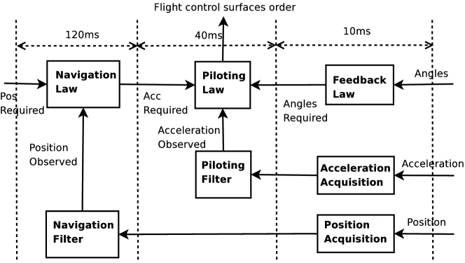
Figure 1: Flight control system

The three sub-systems are first defined separately by different teams. The integrator then assembles them in the global system and specifies how they communicate. The language focuses on this assembly level.

1.2 Contribution

The main novelties of our approach are: first the integrator can develop the complete system in a unified formal framework (a high-level formal language) and second the language along with its compiler covers the development of the system from its design to its implementation, through automated code generation.

This relies on two different research domains. On the one hand, scheduling theory focuses mainly on satisfying system real-time constraints but usually disregards system functional behaviour. This ensures the correctness of the temporal properties of the system, but makes it hard to verify the functional correctness of the system. In the case of multi-periodic systems, this often leads to non-deterministic process communications. On the other hand, synchronous languages focus on the correctness of the functional behaviour of the system and ensure that it is deterministic. However, classic synchronous languages abstract from real-time (except some recent extensions discussed in Sect. 7), which makes them ill-adapted to the implementation of multi-periodic systems.

Our work combines scheduling theory and synchronous languages to ensure both the functional and the temporal correctness of multi-periodic systems. This is particularly suitable for the implementation of critical systems. The integrator programs the system with the language introduced in [6], which extends synchronous languages with high-level real-time primitives. The compiler then generates the set of real-time tasks corresponding to this program. Tasks are then translated into C threads, each one containing the functional code of a task completed with a deterministic data-exchange protocol that does not require synchronization primitives (such as semaphores). The threads are scheduled concurrently with the EDF policy. They can be preempted by the scheduler during their execution but preemptions do not jeopardize the functional correctness of the system. The use of an EDF scheduler departs from the classic compilation scheme of synchronous languages, which translates a program into a “single-loop” sequential code [8]. The single-loop scheme relies on a static-priority non-preemptive scheduling policy, which makes it ill-adapted for implementing multi-periodic processes. A dynamic-priority preemptive policy like EDF allows to achieve better processor utilization (to execute more time-consuming processes). The complete compilation process has been implemented in OCaml and is about 3000 code lines long. It generates C code with calls to the real-time primitives defined in the real-time extensions of POSIX [14].

1.3 Paper Outline

Sect. 2 gives an overview of the language for specifying multi-periodic systems and shows how the case study can be programmed. We then detail the compilation process. The correctness of the system is first verified by a series of static analyses (Sect. 3). We then translate the program into a set of real-time tasks (Sect. 4). The preservation of the synchronous semantics during inter-task communications is ensured by a buffering protocol described in Sect. 5. We can then translate the tasks into C code for a simple real-time platform (Sect. 6). A comparison with related works is given in Sect. 7.

2 A Synchronous Real-Time Language

2.1 Informal Presentation

We present the language through the programming of the Flight Control System of Fig. 1. The different operations of the Flight Control System are first declared as imported nodes, named after the initials of the operations (for instance, PA stands for “Position Acquisition”):

⬇

imported node PA(i: int) returns (o: int) wcet 1;

imported node AA(i: int) returns (o: int) wcet 1;

…

The declaration of an imported node specifies the inputs and outputs of the node with their types and the worst case execution time (wcet) of the node. For instance, the node PA has one input i of type int, one output o of type int and its wcet is 1.

For each sub-system, we define an intermediate node that groups the operations of the sub-system. Node definitions are modular and hierarchical. There are several ways to decompose the Flight Control System into nodes and it is also possible to program the whole system as a single node. However, the different decompositions produce the same behaviour as intermediate nodes are flattened during the compilation (see Sect. 4.1). We choose to group operations by sub-systems (and by rates) for better readability. In the following, the suffix _o stands for “observed”, _r for “required” and _i for “intermediate”. The node for the acquisition loop is defined as follows:

⬇

node acquisition(angle,pos,acc)returns(pos_i,acc_i,angle_r)

let

pos_i = PA(pos);

acc_i = AA(acc);

angle_r = FL(angle);

tel

This node has three inputs and three outputs, the types of which are left unspecified and will be inferred by the type-checker of the language (see Sect. 3). The body of the node (the let ... tel block) is a set of equations that define how the outputs of the node are computed from its inputs. All the variables and expressions of a program are flows. For example, the constant value $0$ stands for an infinite constant sequence. Nodes are applied point-wisely to their arguments. So, for instance, at each repetition of node acquisition, the output pos_i is obtained by applying node PA to input pos.

Similarly, we define a node for the piloting loop and for the navigation loop:

⬇

node piloting (angle_r, acc_i, acc_r) returns (order)

var acc_o;

let

acc_o = PF(acc_i);

order = PL (angle_r, acc_o, acc_r);

tel

node navigation (pos_i, pos_r) returns (acc_r)

var pos_o;

let

pos_o = NF(pos_i);

acc_r = NL(pos_o,pos_r);

tel

So far, each node could be defined with the existing Lustre language as each sub-system is mono-periodic. For the main node FCS however, we use new primitives to handle rate transitions (when operations of different rates communicate) and to specify the real-time constraints of the different operations:

⬇

node FCS (pos_r: rate (120, 0); angle, pos, acc) returns (order: due 15)

var acc_i, acc_r, angle_r, pos_i;

let

acc_r = navigation(pos_i/^12,pos_r);

order = piloting(angle_r/^4, acc_i/^4, (0 fby acc_r)*^3);

(pos_i, acc_i, angle_r) = acquisition(angle,pos,acc);

tel

When a faster node consumes a flow produced by a slower node, we under-sample the flow using operator $/\;\hat{}\;$. $e/\;\hat{}\;k$ only keeps the first value out of each $k$ successive values of $e$. For instance flow acc_i is under-sampled by factor 4 as its consumer (piloting) is 4 times slower than its producer (acquisition).

For communications from slow to fast operations, we first delay the flow with operator fby. The operator fby inserts a unitary delay: expression $cste$ produces the value $cst$ at its first iteration and then the previous values of $e$ (ie $e$ delayed by the period of $e$). We then over-sample the delayed flow with operator $*\hat{}\;$. $e*\hat{}\;k$ over-samples $e$ by a factor $k$. Each value of $e$ is duplicated $k$ times in the result. For instance the flow acc_r is delayed and then over-sampled by a factor 3 as its consumer (piloting) is 3 times faster than its producer (navigation). We use a delay before over-sampling the flow to avoid reducing the deadline for the production of the flow. In the case of flow acc_r for instance, without a delay the deadline for NL would be lower than 40.

For now, we have only described the ratio between the execution rates of the nodes. The declaration of the node inputs simply specifies that pos_r has clock $(120,0)$ (ie that it has period 120 and phase 0) and all the different rates of the system are deduced from this information by the clock calculus (see Sect. 3). The declaration of output order, imposes a deadline constraint (due 15), which requires it to be produced less than 15ms after the beginning of its period, to respect some external environment constraint. Its period is left unspecified (its inferred value is 40ms). The behaviour of the new operators is illustrated in Fig. 2, in which we give the value of each expression at each repetition of the system.

date	0	10	20	30	40	…
angle_r	$an_{0}$	$an_{1}$	$an_{2}$	$an_{3}$	$an_{4}$	…
angle_r/^4	$an_{0}$				$an_{4}$	…
date	0	40	80	120	160	…
acc_r	$ac_{0}$			$ac_{1}$		…
0 fby acc_r	0			$ac_{0}$		…
(0 fby acc_r)*^3	0	0	0	$ac_{0}$	$ac_{0}$	…

Figure 2: Behaviour of real-time operators

2.2 Formal Definition: Strictly Periodic Clocks

In the synchronous approach, the computations performed by the system are split into a succession of instants, where each instant corresponds to one repetition of the system. The synchronous assumption requires that for each instant, computations end before the end of the instant. Computations can be activated or deactivated at different instants using clocks. Clocks define the temporal behaviour of the program on the logical time scale of instants.

To define formally the real-time operators presented in the previous section, we introduce a new class of clocks called strictly periodic clocks. Given a set of values $\mathcal{V}$, a flow is a sequence of pairs $(v_{i},t_{i})_{i\in\mathbb{N}}$ where $v_{i}$ is a value in $\mathcal{V}$ and $t_{i}$ is a tag in $\mathbb{N}$, such that for all $i$, $t_{i}<t_{i+1}$. The clock of a flow is its projection on $\mathbb{N}$. A tag represents an amount of time elapsed since the beginning of the execution of the program. Each value of a flow must be computed before its next activation: $v_{i}$ must be produced during the time interval $[t_{i},t_{i+1}[$. After precedence encoding, the deadline may actually be less than $t_{i+1}$, this will be detailed in Sect. 4.3.3.

Definition 1.

(Strictly periodic clock). A clock $h=(t_{i})_{i\in\mathbb{N}}$, $t_{i}\in\mathbb{N}$, is strictly periodic if and only if: $\exists n\in\mathbb{N}^{*},\;\forall i\in\mathbb{N},\;t_{i+1}-t_{i}=n$.

$n$ is the period of $h$, denoted $\pi(h)$ and $t_{0}$ is the phase of $h$, denoted $\varphi(h)$.

Definition 2.

The term $(n,p)\in\mathbb{N}^{*}\times\mathbb{Q}^{+}$ denotes the strictly periodic clock $\alpha$ such that $\pi(\alpha)=n$ and $\varphi(\alpha)=\pi(\alpha)*p$

A strictly periodic clock defines the real-time rate of a flow and is uniquely characterized by its phase and by its period. Strictly periodic clocks relate logical time (instants) to real-time. Locally, each flow has its own notion of instant (it must end before its next activation), and globally we can compare flows that do not share the same notion of instants by relating instants to real-time. We introduce periodic clock transformations to formalize such rate transitions:

Definition 3.

Let $\alpha$ be a strictly periodic clock, operations $/_{.},*_{.}$ and $\rightarrow_{.}$ are periodic clock transformations, that produce new strictly periodic clocks satisfying the following properties:

• $\pi(\alpha/_{.}k)=k*\pi(\alpha),\;\varphi(\alpha/_{.}k)=\varphi(\alpha),k\in\mathbb{N}^{*}$

• $\pi(\alpha*_{.}k)=\pi(\alpha)/k,\;\varphi(\alpha*_{.}k)=\varphi(\alpha),k\in\mathbb{N}^{*}$

• $\pi(\alpha\rightarrow_{.}q)=\pi(\alpha),\;\varphi(\alpha\rightarrow_{.}q)=\varphi(\alpha)+q*\pi(\alpha),q\in\mathbb{Q}$

Rate transition operators apply periodic clock transformations to flows. If $e$ has clock $\alpha$, then $e/\;\hat{}\;k$ has clock $\alpha/_{.}k$, $e*\hat{}\;k$ has clock $\alpha*_{.}k$ and $e\sim>q$ has clock $\alpha\rightarrow_{.}q$.

2.3 Syntax

The syntax of the language is close to Lustre. It is extended with real-time primitives based on strictly periodic clocks. The grammar of the language is given in Fig. 3. A program consists of a list of node declarations ($nd$). Nodes can either be defined in the program (node) or implemented outside (imported node), for instance by a C function. Node durations must be provided for each imported node, more precisely an upper bound on worst case execution times ($wcet$). The external code provided for imported nodes can itself be generated by a standard synchronous language compiler (like Lustre), in case developers want to program the whole system using synchronous languages. The clock of input/output parameters ($in/out$) of a node can be declared strictly periodic ($x:rate(n,p)$, $x$ then has clock $(n,p)$) or unspecified ($x$). A deadline constraint can be imposed on outputs ($x:rate(n,p)n^{\prime}$, the deadline is $n^{\prime}$). The body of a node consists of an optional list of local variables ($var$) and a list of equations ($eq$). Each equation defines the value of one or several variables using an expression on flows ($var=e$). Expressions may be immediate constants ($cst$), variables ($x$), pairs ($(e,e)$), initialised delays ($cste$), applications ($N(e)$) or expressions using strictly periodic clocks ($epck$). Values $k$, $n$, $n^{\prime}$, $q$ must be statically evaluable. Value $q$ must be an element of $\mathbb{Q}^{+}$.

$$\begin{array}[]{lcl}cst&::=&\;|\;\;|\;0\;|\;...\\ var&::=&x\;|\;var,var\\ e&::=&cst\;|\;x\;|\;(e,e)\;|\;cste\;|\;N(e)\;|\;epck\\ epck&::=&e/\;\hat{}\;k\;|\;e*\hat{}\;k\;|\;e\sim>q\\ eq&::=&var=e\;|\;eq;eq\\ in&::=&x:rate(n,p)\;|\;x\;|\;in;in\\ out&::=&x:rate(n,p)\;|\;x:rate(n,p)n^{\prime}\;|\;x\;|\;out;out\\ nd&::=&N(in)(out)[var;]{eq}\\ &&\;|\;N(in)(out)n;\end{array}$$

Figure 3: Language grammar

3 Static Analyses

Synchronous languages are targeted for critical systems. Therefore, the compilation process puts strong emphasis on the verification of the correctness of the programs to compile. This consists of a series of static analyses of the program, which are performed before code generation.

The first analysis performed by the compiler is the type-checking. The language is a strongly typed language, in the sense that the execution of a program cannot produce a run-time type error. Each flow has a single, well-defined type and only flows of the same type can be combined. The type-checking of the language is fairly standard [13]. For the example of the Flight Control System, the type-checker produces the flowing type for node FCS: (int*int*int*int)->int. This means that the node takes four integer inputs and produces one integer output. This type is inferred from the types of the imported nodes.

The causality check verifies that the program does not contain cyclic definitions: a variable cannot instantaneously depend on itself (i.e. not without a fby in the dependencies). For instance, the equation x=x+1; is incorrect, it is similar to a deadlock since we need to evaluate x+1 to evaluate x and we need to evaluate x to evaluate x+1.

The clock calculus (defined in [6]) verifies that a program only combines flows that have the same clock. When two flows have the same clock, they are synchronous as they are always present at the same instants. Combining non-synchronous flows leads to non-deterministic programs as we access to undefined values. For instance we can only compute the sum of two synchronous flow, because the value of the sum is ill-defined when only one of the two flows is absent (when the two flows are absent the sum flow is simply absent, which is well-defined). The clock calculus ensures that a synchronous program will never access to undefined values. For the example of the Flight Control System, the clock-calculus produces the following clock for node FCS: ((120,0)*(10,0)*(10,0)*(10,0))->(40,0). This means that inputs angle, acc, position have period 10, while input position_r has period 120. The output order has period 40 (though its deadline is 10). These static analyses ensure that a program accepted by the compiler has a deterministic behaviour.

4 Translation into Real-Time Tasks

This section details how the compilation process translates the input program into a set of real-time tasks. We first extract a task graph from the program, where tasks are related by precedence constraints. We then encode task precedences in task real-time attributes to obtain a set of independent tasks.

4.1 Task Graph Extraction

4.1.1 Tasks

A synchronous program consists of a hierarchy of nodes, the leaves of which are predefined or imported nodes. The task graph generation process first inlines intermediate nodes appearing in the main node recursively, replacing each intermediate node call by its set of equations. For instance, the program of the Flight Control System of Sect. 2.1 is translated into a single node (the main node FCS) containing one node call to each imported node, PA, AA, FL, PF, PL, NF, NL, one node call to operator $*\hat{}\;$, one node call to operator fby and three node calls to operator $/\;\hat{}\;$.

This “flattened” main node is then translated into a task graph. Each imported node call is translated into a task. Each variable of the node and predefined operator call is also translated into a vertex but will later be reduced to simplify the graph (see Sect. 4.1.3). The clustering of several nodes into the same task to reduce the number of generated tasks is beyond the scope of this paper. We could probably reuse existing strategies, for instance those suggested in [4].

4.1.2 Task Precedences

In order to respect the synchronous semantics, for each data-dependency there must be a precedence from the task producing the data to the task consuming it. Task precedences are deduced from data dependencies between expressions of the program. Similarly to [8], we say that an expression $e^{\prime}$ precedes an expression $e$ when $e$ syntactically depends on $e^{\prime}$. This occurs either when $e^{\prime}$ appears in $e$ or when $x$ appears in $e$ and we have an equation $x=e$. Let $g=(V,E)$ denote a task graph, where $V$ is the set of tasks of the graph and $E$ is the set of task precedences of the graph (a subset of $V\times V$). For instance, the flattened Flight Control program contains the two equations pos_o=NF(pos_i/^12); pos_i=PA(pos);. These equations produce the following graph: $(\{$NF,PA,/^12,pos,pos_i,pos_o$\}$, $\{$pos$\rightarrow$ PA, PA$\rightarrow$ pos_i, pos_i$\rightarrow$ /^12, /^12$\rightarrow$ NF, NF $\rightarrow$ pos_o$\})$.

4.1.3 Task Graph Reduction

We then simplify the intermediate graph structure. First, each input of the main node is translated into a (sensor) task and each output of the main node is translated into a (actuator) task. Second, we remove variables from the graph, replacing recursively each pair of precedence $N\rightarrow x\rightarrow M$, where $x$ is a local variable, by a single precedence $N\rightarrow M$.

We finally translate predefined nodes into precedence annotations. A precedence $\tau_{i}\stackrel{{\scriptstyle\tiny ops}}{{\rightarrow}}\tau_{j}$ represents an extended precedence, where $ops$ is a list of precedence annotations $op$, with $op\in\{*\hat{}\;k,/\;\hat{}\;k,\sim>q,\mbox{\tt fby}\}$. $op.ops$ denotes the list whose head is $op$ and whose tail is $ops$ and $\epsilon$ denotes the empty list. For instance, the precedences PA$\rightarrow$ pos_i, pos_i$\rightarrow$ /^12, /^12$\rightarrow$ NF are simplified into a single extended precedence PA$\stackrel{{\scriptstyle\tiny/\;\hat{}\;12}}{{\rightarrow}}$NF. When the rewriting terminates, every task of the graph corresponds to either an imported node or a sensor or an actuator. The reduced task graph of the Flight Control System is given in Fig. 4.

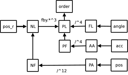
Figure 4: Reduced task graph for the Flight Control System program

4.2 Real-Time Characteristics Extraction

Each task $\tau_{i}$ of the graph is characterized by its real-time attributes $(T_{i},C_{i},r_{i},d_{i})$. $\tau_{i}$ is instantiated periodically with period $T_{i}$. It cannot start its execution before all its predecessors, defined by the precedence constraints, complete their execution. $C_{i}$ is the (worst case) execution time of the task. $r_{i}$ is the release date of the first instance of the task. The subsequent release dates are $r_{i}+T_{i}$, $r_{i}+2T_{i}$, etc. $d_{i}$ is the relative deadline of the task. The absolute deadline $D_{i}[j]$ of the instance $j$ of a task $\tau_{i}$ is the release date $R_{i}[j]$ of this instance plus the relative deadline of the task: $D_{i}[j]=R_{i}[j]+d_{i}$. Task real-time characteristics are extracted as follows:

• Periods: The period of a task is obtained from its clock $ck_{i}$. We have $T_{i}=\pi(ck_{i})$.

• Deadlines: By default, the deadline of a task is its period ($d_{i}=T_{i}$). Deadline constraints can also be specified on the production of a node output (o: due n).

• Release Dates: The initial release date of a task is the phase of its clock: $r_{i}=\varphi(ck_{i})$.

• Execution Times: The execution time $C_{i}$ of a task is directly specified by the wcet of the imported node declaration. For simplification, we consider that the run-time overhead due to task preemptions is negligible.

4.3 Precedence Encoding

4.3.1 Simple Precedences Encoding

[3] showed that a set of dependent tasks (task related by precedence constraints) can be reduced to a set of independent ones (without precedences) obtaining an equivalent problem under the EDF policy, by adjusting task release dates and deadlines such that precedences are encoded in the adjusted real-time characteristics. The adjusted absolute deadline $D^{*}_{i}$ of a task is:

$$D^{*}_{i}=\min_{\tau_{j}\in succ(\tau_{i})}(D_{i},min(D^{*}_{j}-C_{j}))$$

If we want to perform a schedulability test, the adjusted release date of a task is:

$$R^{*}_{i}=\max_{\tau_{j}\in pred(\tau_{i})}(R_{i},max(R^{*}_{j}+C_{j}))$$

If we only want to schedule the program correctly, the adjusted release date of a task $R^{*^{\prime}}_{i}$ is:

$$R^{*^{\prime}}_{i}=\max_{\tau_{j}\in pred(\tau_{i})}(R_{i},max(R^{*^{\prime}}_{j}))$$

For simplification, we only consider the second encoding in the following.

4.3.2 Extended Precedences Encoding

Fig. 5, shows that we can unfold extended precedences between tasks into simple precedences between task instances. The precedence encoding technique can then be applied to the “unfolded” graph.

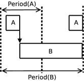
(a) $A\stackrel{{\scriptstyle\tiny/\;\hat{}\;2}}{{\rightarrow}}B$

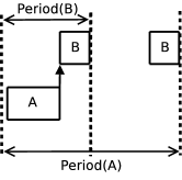
(b) $A\stackrel{{\scriptstyle\tiny*\hat{}\;2}}{{\rightarrow}}B$

(c) $A\stackrel{{\scriptstyle\tiny\mbox{\tt fby}}}{{\rightarrow}}B$

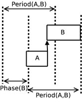
(d) $A\stackrel{{\scriptstyle\tiny\sim>1/2}}{{\rightarrow}}B$

Figure 5: Encoding extended precedences

More formally, let $\tau_{i}[n]\rightarrow\tau_{j}[n^{\prime}]$ denote a precedence from task instance $\tau_{i}[n]$ to task instance $\tau_{j}[n^{\prime}]$. From the semantics of predefined operators, we have $\tau_{i}\stackrel{{\scriptstyle\tiny ops}}{{\rightarrow}}\tau_{j}\Rightarrow\forall n,\;\tau_{i}[n]\rightarrow\tau_{j}[g_{ops}(n)]$, with $g_{ops}$ defined as follows:

$$g_{*\hat{}\;k.ops}(n)=g_{ops}(kn) g_{/\;\hat{}\;k.ops}(n)=g_{ops}(\lceil n/k\rceil)$$

$$g_{\sim>q.ops}(n)=g_{ops}(n) g_{\tiny\mbox{\tt fby}.ops}(n)=g_{ops}(n+1)$$

$$g_{\epsilon}(n)=n$$

The precedence relation is an over-approximation of the data-dependency relation. Indeed, there is a data dependency between $\tau_{i}[n]$ and $\tau_{j}[n^{\prime}]$, meaning that $\tau_{j}[n^{\prime}]$ consumes the data produced by $\tau_{i}[n]$, if and only if $\tau_{i}\stackrel{{\scriptstyle\tiny ops}}{{\rightarrow}}\tau_{j}\wedge n^{\prime}=g_{ops}(n)\wedge g_{ops}(n)\neq g_{ops}(n+1)$.

We can then adapt the encoding to our context. For each precedence $\tau_{i}\stackrel{{\scriptstyle\tiny ops}}{{\rightarrow}}\tau_{j}$, we must adjust the release dates and deadlines of each instance $\tau_{i}[n]$ such that $R^{*}_{i}[n]\leq R^{*}_{j}[g_{ops}(n)]$ and $D^{*}_{i}[n]\leq D^{*}_{j}[g_{ops}(n)]-C_{j}$. Concerning release dates, we can easily prove that thanks to the synchronous semantics we already have $R_{i}[n]\leq R_{j}[g_{ops}(n)]$, so release dates do not need to be adjusted. Concerning deadlines, we need to transpose the formulae to relative deadlines to fit our task model. From the definition of relative deadlines: $D^{*}_{i}[n]\leq D^{*}_{j}[g_{ops}(n)]-C_{j}\Leftrightarrow d_{i}[n]\leq d_{j}[g_{ops}(n)]+r_{j}+g_{ops}(n)T_{j}-r_{i}-nT_{i}-C_{j}$.

4.3.3 Deadline Calculus

In practice we do not need to unfold extended precedences to perform their encoding. Instead, we represent the sequence of deadlines of the instances of a task as a finite repetitive pattern called deadline word. A unitary deadline specifies the relative deadline for the computation of a single instance of a task. It is simply an integer value $d$. A deadline word defines the sequence of unitary deadlines for each instance of a task. The set of deadline words is defined by the following grammar: $w::=(u)^{\omega}\;\;u::=d\;|\;d.u$. Term $(u)^{\omega}$ denotes the infinite repetition of word $u$. In the following, $w[n]$ denotes the $n^{th}$ unitary deadline of deadline word $w$ ($n\in\mathbb{N}$).

Let $w_{i}$ denote the deadline word of task $\tau_{i}$. A precedence $\tau_{i}\stackrel{{\scriptstyle\tiny ops}}{{\rightarrow}}\tau_{j}$ is encoded by a constraint relating $w_{i}$ to $w_{j}$ of the form:

$$w_{i}\leq W_{ops}(w_{j})+\Delta_{ops}(T_{i},T_{j})-C_{j}+r_{j}-r_{i}$$

where, for all $n$, $W_{ops}(w_{j})[n]=w_{j}[g_{ops}(n)]$ and $\Delta_{ops}(T_{i},T_{j})[n]=g_{ops}(n)T_{j}-nT_{i}$.

Let $\psi_{ops}(\tau_{j})=W_{ops}(w_{j})+\Delta_{ops}(T_{i},T_{j})-C_{j}+r_{j}-r_{i}$.

Property 1.

$\Delta_{ops}(T_{i},T_{j})$ is periodic and can be represented as a deadline word. The set of deadline words is closed under operation $W_{ops}$ and under deadline words addition. As a consequence, $\psi_{ops}(\tau_{j})$ is a deadline word.

Proof.

By induction. ∎

Property 2.

The deadline words of a task graph $g=(V,E)$ can be computed with complexity $\mathcal{O}(|V|+|E|*|w_{max}|)$, where $w_{max}$ denotes the deadline word which has the longest size in the task graph.

Proof.

A reduced task graph is a DAG (when we do not consider delayed precedences), so we can compute the deadline words of the graph by performing a topological sort working backwards (starting from the end of the graph). As the complexity of a topological sort is $\mathcal{O}(|V|+|E|)$, the complexity of the algorithm is $\mathcal{O}(|V|+|E|*|w_{max}|)$ where $w_{max}$ denotes the longest deadline word in the task graph. ∎

For instance, for the Flight Control System program, we take $C_{PA}=1$, $C_{AA}=1$, $C_{FL}=3$, $C_{PF}=4$, $C_{PL}=6$, $C_{NL}=20$, $C_{NF}=5$. To simplify, we take null durations for sensors and actuators. The result of the deadline calculus is: $w_{PA}=(10)^{\omega}$, $w_{AA}=(5.10.10.10)^{\omega}$, $w_{FL}=(9.10.10.10)^{\omega}$, $w_{PF}=(9)^{\omega}$, $w_{PL}=(15)^{\omega}$, $w_{NL}=(120)^{\omega}$, $w_{NF}=(100)^{\omega}$. The deadline words of tasks AA and PA state that, each first repetition out of four successive repetitions the two tasks have a shorter deadline as PF and PL execute. Notice that if we set deadline $5$ for all the instances of AA (instead of a deadline word), this example is not schedulable.

5 Communication Protocol

As task precedences are encoded in task deadlines, inter-task communications do note require synchronization primitives (like semaphores for instance). Indeed, as long as tasks respect their deadlines, data is produced before being consumed, so tasks simply read from and write to some communication buffers allocated in a global shared memory when they execute. However, to respect the synchronous semantics, the input of a task must not change during its execution. Therefore, we propose a communication scheme, which ensures that the input of a task remains available until its deadline.

For a precedence $\tau_{i}\stackrel{{\scriptstyle\tiny ops}}{{\rightarrow}}\tau_{j}$, data produced by $\tau_{i}[n]$ may be consumed by $\tau_{j}[g_{ops}(n)]$ after $\tau_{i}[n+1]$ has started. This is illustrated in Fig. 6, which shows the schedule of two tasks related by extended precedences. Vertical lines on the time axis represent task periods and marks represent task preemptions. An arrow from $A$ at date $t$ to $B$ at date $t^{\prime}$ means that task $B$ may read at time $t^{\prime}$ from the value produced by $A$ at time $t$. In Fig. 6(a), 6(c) and 6(d), when $A[1]$ executes, it must not overwrite the data produced by $A[0]$ because it is consumed by $B[0]$ and $B[0]$ is not complete yet. Therefore, we need a buffer to keep the value of $A[n]$ after $A[n+1]$ has started. In Fig. 6(b), the same data is consumed several times but $A[1]$ can freely overwrite the data produced by $A[0]$, so no specific communication scheme is required.

(a) $A\stackrel{{\scriptstyle\tiny/\;\hat{}\;2}}{{\rightarrow}}B$

(b) $A\stackrel{{\scriptstyle\tiny*\hat{}\;2}}{{\rightarrow}}B$

(c) $A\stackrel{{\scriptstyle\tiny\mbox{\tt fby}}}{{\rightarrow}}B$

(d) $A\stackrel{{\scriptstyle\tiny\sim>1/2}}{{\rightarrow}}B$, $A\stackrel{{\scriptstyle\tiny*\hat{}\;4}}{{\rightarrow}}C$

Figure 6: Communications for extended precedences

The communication protocol allocates a buffer for each extended precedence of the graph. The producer of the data writes to the buffer only if $g_{ops}(n)\neq g_{ops}(n+1)$ (see the definition of data-dependencies in Sect. 4.3). The consumer simply reads from this buffer each time it executes. We allocate a double-buffer when the precedence contains a fby or a $\sim>$, to keep the previous and the current value of the data. This communication scheme is illustrated in more details in Sect. 6.1. It is of course not optimal because in many cases when we consider a set of precedences from a single task $\tau_{i}$ to several tasks $\tau_{j}$ we can use the same communication buffer for some of the tasks $\tau_{j}$. Optimization will be treated in future work, we could for instance adapt the communication scheme proposed by [16] to our language.

6 Code Generation

The compiler generates C code with calls to the real-time primitives defined in the real-time extensions of the POSIX standard (POSIX.13 [14]). The code generation can easily be adapted to any real-time operating system that provides dynamic priority scheduling. Each task is translated into a thread and the threads are executed concurrently by an EDF scheduler modified to handle deadline words.

6.1 Task Code Generation

The generated code consists of a single C file. The file starts with the declaration of one global variable for each communication buffer. For instance, for the communication from PF to PL (acc_o before graph expansion), we have the declaration: int PF_o_PL_i1 (named after the output of the producer and the input of the consumer). For the communication from PL to FL, we have the declaration: int PL_o_FL_i2[2], as there is a delay between the two tasks.

The file then contains a function for each task of the task set. The function mainly consists of an infinite loop, that wraps the function of the corresponding imported node with the code of the communication protocol. One step of the loop corresponds to the execution of one instance of the task. Once buffer updates are complete, the function signals to the scheduler that the current task instance completed its execution so that it can schedule another task.

For instance, the function for task PL is given in Fig. 7. The value returned by the external function PL is a single integer so we can directly assign its return value to an integer variable. When the external function returns a tuple, the output value is returned as a struct pointer in the parameters of the function. The variable NL_o_PL_i3 is the communication buffer for precedence $NL\stackrel{{\scriptstyle\tiny.*\hat{}\;3}}{{\rightarrow}}PL$. It is an array of size 2 as the precedence contains a delay. The delay is initialised at the beginning of the function. PL alternatively reads from value 1 and from value 0 of the array, starting with value 1 (NL_o_PL_i3[(instance+1)%2]). PL then copies its output value to the communication buffer PL_o_order for precedence $PL\rightarrow order$. Instruction invoke_scheduler(0) signals the completion of the task instance.

⬇

void *PL_fun(void * arg) {

NL_o_PL_i3[1]=0; int instance=0;

while (1) {

PL_o = PL(FL_o_PL_i1,PF_o_PL_i2, NL_o_PL_i3[(instance+1)%2]);

PL_o_order=PL_o;

instance++;

invoke_scheduler (0);

}

}

Figure 7: Code generated for task PL

The functions for tasks FL and NL, which produce data used by PL are given in Fig. 8. Variable FL_o_PL_i1 is the communication buffer for precedence $FL\stackrel{{\scriptstyle\tiny/\;\hat{}\;4}}{{\rightarrow}}PL$. It is updated once every 4 iterations, (update_FL_o_PL_i1[instance%4]). For precedence $NL\stackrel{{\scriptstyle\tiny.*\hat{}\;3}}{{\rightarrow}}PL$, NL alternatively copies its output value to the value 0 and to the value 1 of the buffer NL_o_PL_i3.

⬇

void *FL_fun(void * arg) {

int update_FL_o_PL_i1[4]={1,0,0,0}; int instance=0;

while (1) {

FL_o = FL(angle_FL_i1);

if(update_FL_o_PL_i1[instance%4])

FL_o_PL_i1=FL_o;

instance++;

invoke_scheduler (0);

}

}

void *NL_fun(void * arg) {

int instance=0;

while (1) {

NL_o = NL(NF_o_NL_i1,pos_r_NL_i2);

NL_o_PL_i3[instance%2]=NL_o;

instance++;

invoke_scheduler (0);

}

}

Figure 8: Code generated for tasks FL and NL

The main function then creates one thread for each task, initializes the EDF scheduler and attaches the threads to it. For instance, the thread for task PL is created by the following function call: pthread_create(&tPL,&attrPL,PL_fun,
NULL). tPL is the thread created for this task. attrPL contains the real-time attributes of the task. PL_fun is the function executed by the thread. The last parameter NULL stands for the arguments of PL_fun.

6.2 Implementing EDF with Variable Deadlines

We choose to prototype the scheduler using MaRTE Operating System [15], which was designed specifically to ease the implementation of application-specific schedulers while remaining close to the POSIX model. We modify the EDF scheduler provided with the OS to support deadline words. To summarize, the EDF scheduler is defined as a high-priority thread created by the main function of the file. The scheduler thread is itself scheduled by the kernel of the OS. It becomes active only when scheduling actions must be taken, which is when the following scheduling events (implemented by means of signals) occur: the current instance of a task completes its execution or a new task instance is released. The scheduler then computes the most urgent task among the ready tasks (tasks released and not complete yet), resumes the execution of the corresponding thread where it stopped and suspends the execution of the currently executing thread, if any. The scheduler thread then becomes inactive until the next scheduling event.

The support of deadline words requires very few modifications. We define deadline words and modify the structure describing task real-time attributes as shown in Fig. 9. Then, we modify the function that programs the next instance of a task when the current instance completes. For a task $\tau_{i}$, the attributes of which are described by the value t_data, the release date and the deadline of its new instance are computed as described in Fig. 10 ($D_{i}[n]=R_{i}[n]+d_{i}[n]$). The function incr_timespec(t1,t2) increments t1 by t2 and the function (t1,t2,t3) sets t1 to t2+t3.

⬇

typedef struct dword { struct timespec *dds; int wsize; } dword_t;

typedef struct thread_data {

struct timespec period;

struct timespec initial_release;

dword_t dword;

struct timespec next_deadline;

struct timespec next_release;

int instance;

} thread_data_t;

Figure 9: Data type representing task real-time attributes

⬇

dword_t dw = t_data->dword; t_data->instance++;

incr_timespec (&t_data->next_release,&t_data->period);

add_timespec (&t_data->next_deadline,&t_data->next_release,

&(dw.dds[t_data->instance%dw.wsize]));

Figure 10: Releasing a new task instance

We can see that the overhead due to the support of deadline words remains very reasonable. Altogether, we modified about 20 lines of code of the original EDF scheduler, which is 300 lines of code long. We compiled and executed the C code generated for the Flight Control System and it behaved as expected.

7 Related Works

The language used in this article relies on a specific class of clocks to handle the multi-periodic aspects of a system. Real-time periodic clocks have also been introduced in [4], but they do not include clock transformations to efficiently handle rate transitions. Our rate-transition operators are also very similar to the rate transition blocks of Simulink [11]. Yet, as far as we know, for models using such blocks, the code generation tool (Real-Time Workshop) relies on a Rate-Monotonic scheduler [10] used with semaphores to handle task communications, which is not an optimal scheduling policy for this scheduling problem.

The scheduling of multi-rate Synchronous Data Flow (SDF) is a well studied problem (see for instance [9, 17, 12]). In particular [17] studies the implementation of SDF with a dynamic scheduler using preemption. However, though multi-rate systems are at the chore of SDF graphs, SDF operations are not periodic, they are not released periodically and their relative deadline is not their period. As a consequence, these results do not apply to our problem.

[16] deals with the execution of a set of synchronous tasks, the semantics of which is very close to our task sets, with a dynamic scheduler. However, the authors do not detail how the synchronous task set is obtained, for instance how it is translated from a synchronous language, and task precedences are not specified in the task set.

A simple solution to the problem of scheduling tasks related by extended precedences is to unfold the extended precedence graph on the hyperperiod of the tasks and use [3] to encode the simple precedences of the unfolded graph. This solution replaces each task $\tau_{i}$ by $HP/T_{i}$ duplicates (where $HP$ is the hyperperiod of the tasks) in the unfolded graph. This can lead to important computation overhead at execution as the scheduler needs to make its decisions according to a task set that will contain many tasks. Our solution does not duplicate any task, so the scheduler takes less time to make its decisions.

8 Conclusion

We proposed a language for programming critical systems with multiple real-time constraints, along with its compiler, which automatically translates a program into a set of independent real-time tasks programmed in C with POSIX.13 real-time extensions. The generated code is schedulable optimally by a slightly modified EDF scheduler and requires no synchronization primitives. Though tasks are scheduled concurrently and preemptions are allowed, the generated program respects the real-time and the functional semantics of the original program.

References

- [1]
- [2] Albert Benveniste, Paul Le Guernic & Christian Jacquemot (1991): Synchronous programming with events and relations: the Signal language and its semantics. Sci. of Compu. Prog. 16(2).
- [3] Houssine Chetto, Marilyne Silly & T. Bouchentouf (1990): Dynamic Scheduling of Real-Time Tasks under Precedence Constraints. Real-Time Systems 2.
- [4] Adrian Curic (2005): Implementing Lustre programs on distributed platforms with real-time constraints. Ph.D. thesis, Université Joseph Fourier, Grenoble.
- [5] Julien Forget (2009): A Synchronous Language for Critical Embedded Systems with Multiple Real-Time Constraints. Ph.D. thesis, Université de Toulouse - ISAE/ONERA, Toulouse, France.
- [6] Julien Forget, Frédéric Boniol, David Lesens & Claire Pagetti (2008): A Multi-Periodic Synchronous Data-Flow Language. In: 11th IEEE High Assurance Systems Engineering Symposium (HASE’08), Nanjing, China, pp. 251 – 260.
- [7] Nicolas Halbwachs, Paul Caspi, Pascal Raymond & Daniel Pilaud (1991): The synchronous data-flow programming language LUSTRE. Proceedings of the IEEE 79(9).
- [8] Nicolas Halbwachs, Pascal Raymond & Christophe Ratel (1991): Generating efficient code from data-flow programs. In: Third International Symposium on Programming Language Implementation and Logic Programming (PLILP ’91), Passau, Germany, pp. 207–218.
- [9] Edward Lee & David Messerschmitt (1987): Static scheduling of synchronous dataflow programs for digital signal processing. IEEE Transaction on Computer C(36).
- [10] Cheng L. Liu & James W. Layland (1973): Scheduling algorithms for multiprogramming in a hard-real-time environment. Journal of the ACM 20(1).
- [11] The Mathworks: Simulink: User’s Guide.
- [12] Hyunok Oh, Nikil Dutt & Soonhoi Ha (2006): Memory optimal single appearance schedule with dynamic loop count for synchronous dataflow graphs. In: Asia and South Pacific Design Automation Conference (ASP-DAC’06), Yokohama, Japan, pp. 497 – 502.
- [13] Benjamin C. Pierce (2002): Types and programming languages. MIT Press, Cambridge, USA.
- [14] POSIX.13 (1998): IEEE Std. 1003.13-1998. POSIX Realtime Application Support (AEP). The Institute of Electrical and Electronics Engineers.
- [15] Mario A. Rivas & Michael G. Harbour (2002): POSIX-Compatible Application-Defined Scheduling in MaRTE OS. In: 14th Euromicro Conference on Real-Time Systems (ECRTS’02), Washington, USA, p. 67.
- [16] Stavros Tripakis, Christos Sofronis, Paul Caspi & Adrian Curic (2005): Translating discrete-time Simulink to Lustre. ACM Trans. Embed. Comput. Syst. 4(4).
- [17] Dirk Ziegenbein, Jan Uerpmann & Rolf Ernst (2000): Dynamic response time optimization for SDF graphs. In: IEEE/ACM international conference on Computer-aided design (ICCAD’00), San Jose, USA, pp. 135–141.