Granular Scale Magnetic Flux Cancellations in the Photosphere

Abstract

We investigate the evolution of 5 granular-scale magnetic flux cancellations just outside the moat region of a sunspot by using accurate spectropolarimetric measurements and G-band images with the Solar Optical Telescope aboard Hinode. The opposite polarity magnetic elements approach a junction of the intergranular lanes and then they collide with each other there. The intergranular junction has strong red shifts, darker intensities than the regular intergranular lanes, and surface converging flows. This clearly confirms that the converging and downward convective motions are essential for the approaching process of the opposite-polarity magnetic elements. However, motion of the approaching magnetic elements does not always match with their surrounding surface flow patterns in our observations. This suggests that, in addition to the surface flows, subsurface downward convective motions and subsurface magnetic connectivities are important for understanding the approach and collision of the opposite polarity elements observed in the photosphere. We find that the horizontal magnetic field appears between the canceling opposite polarity elements in only one event. The horizontal fields are observed along the intergranular lanes with Doppler red shifts. This cancellation is most probably a result of the submergence (retraction) of low-lying photospheric magnetic flux. In the other 4 events, the horizontal field is not observed between the opposite polarity elements at any time when they approach and cancel each other. These approaching magnetic elements are more concentrated rather than gradually diffused, and they have nearly vertical fields even while they are in contact each other. We thus infer that the actual flux cancellation is highly time dependent events at scales less than a pixel of Hinode SOT (about 200 km) near the solar surface.

1 INTRODUCTION

The magnetic fields in the photosphere are highly heterogeneous, as is well known (e.g. Parker, 1979; Zwaan, 1987; Stenflo, 1989). These fields exist in a dynamical state in a spectrum of sizes, ranging from the kilo-gauss fibrils with diameters of a few hundred kilo-meters, through the mesoscale pores, to sunspots of various sizes. In the turbulent convection zone immediately below the quiet-Sun photosphere, the magnetic field is dominated by the fluid. Therefore, it is expected that the field distribution is organized into the convective cells. This field distribution is necessarily complex with flux connectivities of various scales, across individual and multiple cells. Magnetic concentrations that have vertical and strong (kilo-gauss) field are observed along the boundaries of the convective cells. A most prominent feature in the quiet Sun is the network magnetic field that partially outlines supergranular cells. It is believed that the network magnetic field is formed by the advection of internetwork fields via the supergranular flows. Magnetic elements in internetwork areas tend to move toward the nearest network concentration at a speed of about 0.2 km s^-1 (de Wijn et al., 2008), and their rms velocity is about 1.5 km s^-1 in internetwork areas (Nisenson et al., 2003; de Wijn et al., 2008). Velocities of 0.2 km s^-1 and 1.5 km s^-1 are similar to a typical speed of supergranular flows and granular flows, respectively.

Down at the scales of a few hundred kilo-meters, equal to a few photospheric density scale heights, magnetic elements of both polarities form to often merge and collide with each other in the photospheric fluid. The net magnetic flux increases or decreases, depending on whether like-polarity or opposite-polarity magnetic elements have merged. In this paper, we report an interesting set of “magnetic flux cancellation” events of this kind observed at the high spatial resolution of the Solar Optical Telescope (SOT; Tsuneta et al., 2008) aboard Hinode (Kosugi et al., 2007). The magnetic flux cancellation is a descriptive term to indicate a mutual flux loss due to the apparent collision of the opposite-polarity magnetic elements (Martin, Livi, & Wang, 1985). This flux cancellation is essential to the process of replacement of old magnetic flux with newly emerging flux in the quiet Sun on a timescale of a few days (Schrijver et al., 1997; Hagenaar, 2001), and also to the process of removal of sunspot magnetic flux from the photosphere (Kubo et al., 2008).

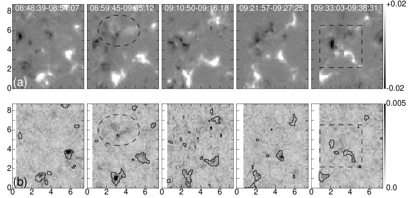
Figure 2: Time series of (a) the total circular polarization ($C_{tot}$) and (b) the total linear polarization ($L_{tot}$) before the flux cancellation in Region A of Figure 1. White (black) indicates positive (negative) polarity in panel a. The contours in panel b represent the $\pm 0.01C_{tot}$ levels. The units of vertical and horizontal axes are in arcseconds. The dashed circle indicates a flux emerging site. The dashed box in the final frame includes our target flux cancellation event, and is identical to the field of view of Fig. 3.

Various possible processes have been proposed to explain the observed flux cancellation (e.g. Zwaan, 1987; Ryutova et al., 2003), involving submergence (retract) of $\Omega$-shaped loops or emergence of U-shaped loops across the photosphere. In both cases, the canceling opposite-polarity magnetic elements correspond to the two intersections of such loops with the photospheric layer. The opposite-polarity magnetic elements disappear when the top of a submerging $\Omega$-loop has passed through the photospheric layer (see Fig.2 in Zwaan, 1987). Alternatively, these elements disappear when the bottom of a rising U-loop has passed clear through the photospheric layer. When magnetic field lines have emerged into the chromosphere and corona, they can hardly submerge back below the photosphere because of magnetic buoyancy. Magnetic reconnection taking place within several scale heights above the solar surface is probably needed to create low-lying $\Omega$-loops whose magnetic tension force can then overcome the magnetic buoyancy force (Parker, 1975). In the photospheric magnetic reconnection cases, reconnection should be most efficient around the temperature minimum region: about 600 km above the solar surface (Litvinenko, 1999; Takeuchi & Shibata, 2001). In contrast, both magnetic tension and buoyancy forces are directed upward in the case of a U-loop rising through the photosphere. Magnetic reconnection is therefore not crucial for the emerging U-loops.

An important observable signature for understanding flux cancellation is the motion of the horizontal magnetic field connecting the canceling magnetic elements. Horizontal magnetic fields have been observed between the opposite-polarity magnetic elements during the cancellations of moving magnetic features around a sunspot (Chae et al., 2004). Similar horizontal fields have also been observed in events of cancellations of pores and sunspots (Kubo & Shimizu, 2007). A flux cancellation without increase of the horizontal field has also been reported for the moving magnetic features (Bellot Rubio & Beck, 2005). Knowledge of the full vector field permits one to determine whether the field geometry has $\Omega$-loop topology or U-loop topology, but in the case of cancellation of small, isolated flux elements, such a determination is often compromised by usual difficulty of resolving the 180$\arcdeg$ azimuth ambiguity. Regarding the motions at such a cancellation site, Harvey et al. (1999) show that the magnetic flux disappears in the chromosphere before it does in the photosphere for at least about half of the cancellation events. They suggest that magnetic flux is submerging in most, if not all, of the cancellation sites. On the other hand, both Doppler red shift (Chae et al., 2004) and Doppler blue shift (Yurchyshyn & Wang, 2001) are reported in the cancellation sites. The center-to-limb variations of the Doppler velocities at the polarity inversion lines in the cancellation sites suggest that the observed velocities with the spatial resolution of about 1$\arcsec$ mainly show the gas flows along the horizontal fields rather than actual emerging or submerging motions of the field lines (Kubo & Shimizu, 2007). Observationally, the physical process of the magnetic flux cancellation is still not well understood.

Recent observations with the high spatial resolution by Hinode SOT show that downward motions (red-shifts) are continuously observed during the flux cancellation process (Iida et al., 2010). From the Stokes-V signals far from the disk center, they also suggest that the canceling opposite polarity elements tend to have an $\Omega$-shaped configuration rather than a U-shaped configuration. In this paper, we investigate the detailed evolution of canceling magnetic elements and their surrounding convective motions near the disk center by using vector magnetic fields and velocity fields observed with the SOT. We are particularly interested in the evolution that precedes the cancellation in order to investigate why the opposite-polarity magnetic elements approach and collide with each other. For a full understanding of the phenomenon, this dynamical development is as important as the flux removal process at the cancellation site.

2 OBSERVATIONS AND ANALYSIS

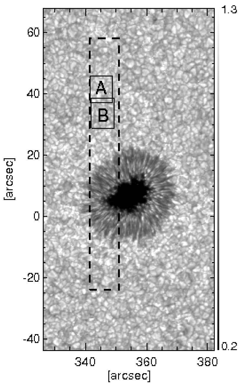
Figure 1: G-band image taken at 08:00:32 on 2007 March 2. The G-band image is normalized to the mean intensity of the quiet area outside the sunspot. The dashed box shows a scan area by the Hinode SP. The solid boxes labeled “A” and “B” are identical to the fields of view of Figs. 2 and 5, respectively.

Our target flux-cancellation events occurred just outside an active region NOAA 10944, as shown by the solid boxes in Figure 1. We selected a data set simultaneously taken by the SOT spectropolarimeter (SP) and filtergraph (FG) in their full spatial resolution modes. The SP repeatedly scanned the same area with a field of view of $10\arcsec\times 82\arcsec$ (the dotted box in Fig. 1) for 4.5 hr from 06:35:32 on 2007 March 2. The SP measured Stokes I, Q, U, and V profiles across Fe I 630.1 nm and 630.2 nm lines. A width of a slit was $0\arcsec.15$ and a pixel sampling along the slit was $0\arcsec.16$. One scan took 5.5 minutes with an integration time of 4.8 s at each slit position. We estimated total circular polarization ($C_{tot}$) and total linear polarization ($L_{tot}$) as follows:

$$C_{tot}=\frac{\int_{\lambda_{0}-21.6\thinspace\textrm{\scriptsize{pm}}}^{\lambda_{0}-4.32\thinspace\textrm{\scriptsize{pm}}}V(\lambda)\,d\lambda}{I_{c}\int_{\lambda_{0}-21.6\thinspace\textrm{\scriptsize{pm}}}^{\lambda_{0}-4.32\thinspace\textrm{\scriptsize{pm}}}\,d\lambda},$$ (1)

$$L_{tot}=\frac{\int_{\lambda_{0}-21.6\thinspace\textrm{\scriptsize{pm}}}^{\lambda_{0}+21.6\thinspace\textrm{\scriptsize{pm}}}\sqrt{Q^{2}(\lambda)+U^{2}(\lambda)}\,d\lambda}{I_{c}\int_{\lambda_{0}-21.6\thinspace\textrm{\scriptsize{pm}}}^{\lambda_{0}+21.6\thinspace\textrm{\scriptsize{pm}}}\,d\lambda},\\$$ (2)

where $\lambda_{0}$ is the center of Fe I 630.2 nm line in each pixel, and $I_{c}$ is the local continuum intensity. The continuum intensity is averaged over the Stokes I profile from $\lambda_{0}+43.2$ pm to $\lambda_{0}+64.8$ pm. In the weak field approximations (Jefferies et al., 1989), $C_{tot}$ is proportional to the longitudinal magnetic flux density ($fB_{L}$) and $L_{tot}$ has the relation to the transverse flux density as $L_{tot}\sim fB_{T}^{2}$, where $B_{L}$, $B_{T}$, $f$ are the longitudinal field strength, transverse field strength, and filling factor, respectively. The observed area is located not far from the disk center (S06W21). We can consider the longitudinal and transverse fields to be the vertical and horizontal fields with respect to the solar surface, respectively. In addition to the magnetic field, we compute the Doppler velocity with respect to the average of Doppler velocities in the quiet area.

During the repeated scans by the SP, the FG took a time series of G-band images with a pixel scale of 0$\arcsec$.05448. The cadence is 1 minute, and the field of view is $56\arcsec\times 112\arcsec$. After applying a sub-sonic filter for the time series of G-band images, we estimated granular flow patterns with the local correlation tracking technique (LCT; November & Simon, 1988). The apodization window of the LCT had a Gaussian shape with the FWHM of 32 pixels (1$\arcsec$.7). The LCT flow maps are calculated from the series of G-band images. The cadence of the LCT flow maps is therefore 1 minute. Drift of the image, arising from the correlation tracker (Shimizu et al., 2008), was removed by aligning the sunspot centers in the G-band images at different times. After removing the image drift, both G-band images and flow maps were averaged over the period corresponding to the duration of an SP map (5.5 minutes). The SP maps were aligned to the averaged G-band images at the time closest to the midpoint of the SP maps. The alignment was performed by the image cross-correlation between the averaged G-band images and the SP continuum intensity maps. Thus, the image drift in the time series of the SP maps was removed as well as the G-band images.

3 RESULTS

Here we present the evolution of flux cancellation events in Region A and Region B of Figure 1. We shall henceforth use simplified terminology of calling the positive-polarity and negative-polarity magnetic elements simply as the positive and negative elements, respectively.

3.1 Region A

The first event is an elemental flux cancellation in Region A. Figure 2 shows the developments of this region prior to the start of the cancellation event. Fuzzy positive (white) and negative (black) elements appear within the dashed circle in the map of the total circular polarization ($C_{tot}$). In this circle, an increase of the total linear polarization ($L_{tot}$) is also observed. These results indicate that the opposite-polarity elements emerge into the photosphere as a pair whereas the canceling magnetic elements in the dashed box do not originally emerge as a pair. The emerged negative elements merge together to consolidate into a stronger negative element that subsequently approach and mutually cancel with a positive element. Even when the negative element is close to the positive element, there is only a slight increase of $L_{tot}$ in a part of the region between them.

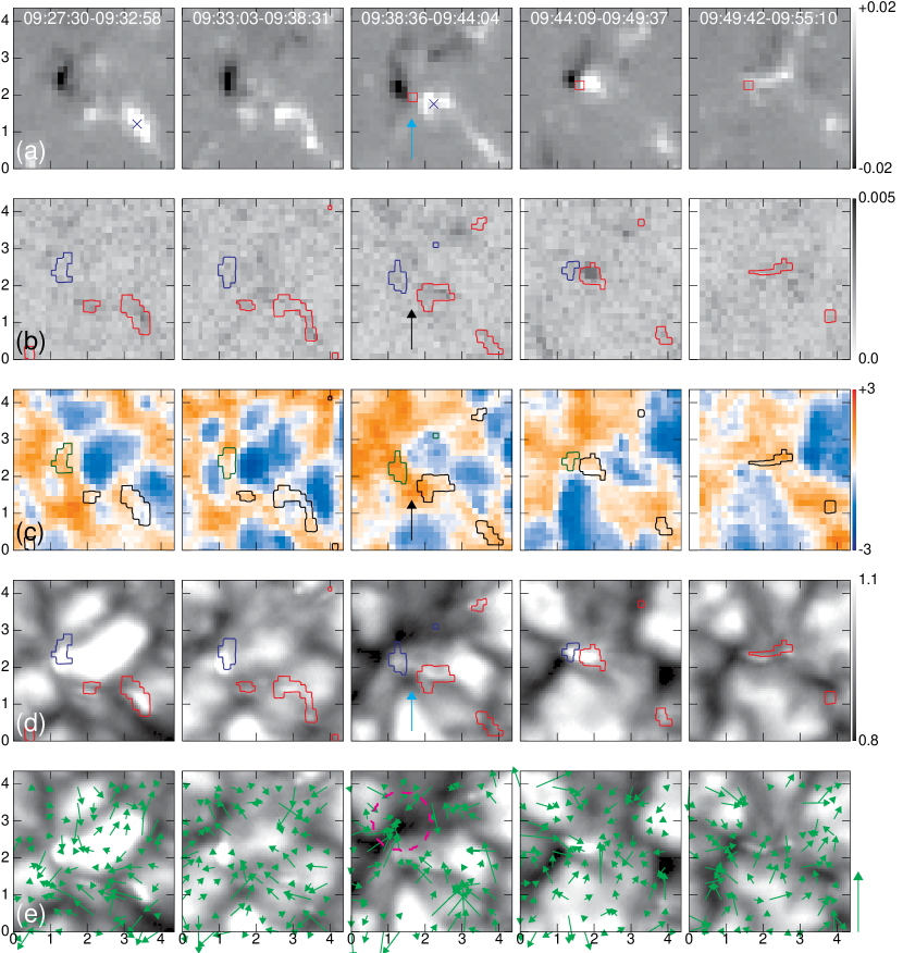
Figure 3: (a) Total circular polarization ($C_{tot}$), (b) total linear polarization ($L_{tot}$), (c) Doppler velocity in units of km s^-1, (d) normalized G-band intensity, and (e) flow map during the flux cancellation in Region A. The upward arrows in panels a-d indicate the strong red-shifted area, and the contours are $\pm 0.01$ of $C_{tot}$. The cross symbols in panel a represent centers of the positive-polarity magnetic element to be canceled. The arrows in panel e show the horizontal velocities derived with the local correlation tracking method. The upward arrow on the right-hand side of the panel is 1.5 km s^-1. The background of panel e is identical to that of panel d, and the dashed circle surrounds the area with strong converging flows.

Figure 3a shows that, like the negative canceling element, smaller positive elements around the cancellation site first converge to form into a prominent positive element that then moves toward the negative element. We trace the center of the positive element. The center (the cross symbol in Fig. 3a) is defined as the average of the position ($\mathbb{r}$) weighted by $C_{tot}$: $\sum{C^{i}_{tot}}\mathbb{r}_{i}/\sum{C^{i}_{tot}}$. This center moves at about 1.4 km s^-1 during 11 minutes. Note that the motion of 1.4 km s^-1 is similar to the rms velocity of magnetic elements in internetwork areas (Nisenson et al., 2003; de Wijn et al., 2008). The positive element collides with the negative magnetic element at a time between the third and fourth frames. The negative element disappears from the photosphere by 10 minutes after the start of the cancellation, whereas the positive element does not completely disappear in this event. Even while the net flux of both negative and positive elements is decreasing, $C_{tot}$ of each pixel in the colliding magnetic elements does not decrease. Furthermore, both $C_{tot}$ and $L_{tot}$ slightly increase at the center of the positive element at the fourth frame in Figure 3. This increase arises from either the increase of the filling factor or the field strength within the positive element. These results suggest that the colliding magnetic elements have nearly vertical magnetic fields until these magnetic elements disappear form the photosphere. On the other hand, no increase of $L_{tot}$ is observed between the canceling opposite polarity elements during the whole flux cancellation process. This means that the horizontal magnetic fields, which are expected in both the submerging $\Omega$-loop model and the emerging U-loop model, do not appear at the cancellation site. Figure 4 confirms that neither Stokes Q nor U signal increases during the flux cancellation.

The cancellation site is located at a junction of the intergranular lanes (the upward arrow in Fig. 3d). The intergranular junction is darker in G-band intensity than its nearby intergranular lanes. Intergranular lanes have generally red shifts, and a larger red shift with about 1.5 km s^-1 is observed at the intergranular junction just before the cancellation (Fig. 3c). Interestingly, such a larger red shift is not observed there during the cancellation. The left panels of Figure 4 also show that the red shift of Stokes I profile is only seen in the top panel taken just before the cancellation. This means that the observed large red shift at the cancellation site does not result from this flux cancellation process. Instead, we may infer that the opposite polarity elements approach the intergranular junction with the large red shift. The intergranular junction tends to have a converging flow rather than a diverging flow, but the flow pattern is not clear in this event. The size of the intergranular junction is too small to examine the flows derived by the LCT method because the LCT window is 1$\arcsec$.7. One interesting result is that the negative element moves toward such a small, less clear converging area although a large, strong converging area with the darker intensity is also located near it, as shown by the dashed circle in Figure 3e.

3.2 Region B

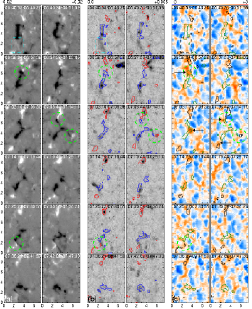
Figure 5: Time series of (a) the total circular polarization ($C_{tot}$), (b) the total linear polarization ($L_{tot}$), and (c) the Doppler velocity. The contours represent the $\pm 0.01C_{tot}$ levels. The dashed circles and the dashed box indicate the flux cancellation sites and the flux emergence site, respectively. The arrows in panel c point to the areas with strong red shifts.

Figure 5 shows a negative element in Region B that evolves into three branches. Each of these three branches elongates toward an area with a large red shift (the arrows in Fig. 5). Magnetic flux cancellations subsequently occur at the tip of each branch (the dashed circles in Fig. 5). An increase of $L_{tot}$ signals indicating horizontal magnetic fields is observed only in the cancellation event enclosed by the final dashed circle. The other 3 cancellation events do not accompany the horizontal magnetic fields, and their properties are similar to the flux cancellation observed in Region A. In the event with the increase of $L_{tot}$, the horizontal fields are located along the intergranular lane with the Doppler red shifts. The sizes of the magnetic elements begin to decrease slightly in the $C_{tot}$ maps just before their collision. This event is different from the other cancellation events: the horizontal field ($L_{tot}$ signals) is already present as a result of the flux emergence well before the event of cancellation sets in, as identified by the dashed box at the beginning of the observation sequence on the top of Figure 5a. This flux emergence has a possibility of distinguishing this event from the other four cancellation events. However, it is unclear whether these horizontal fields are the same as the horizontal fields observed during the cancellation or not, because the $L_{tot}$ signals in the dashed box disappear briefly before the opposite polarity elements approach each other.

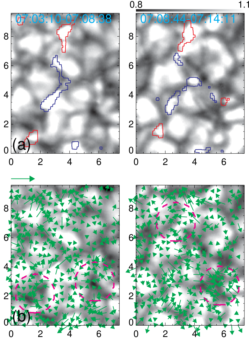
Figure 6: (a) G-band images and (b) flow maps with the local correlation tracking method in Region B. The field of view and the contours are identical to those of the third row in Fig.5. The right-handed arrow at the top of panel b is 1.5 km s^-1. The dashed circles encircle the areas with strong converging flows. The background of panel b is identical to that of panel a.

The circles in Figure 6 show that the areas with strong converging flows mostly have a darker G-band intensity in the intergranular lanes. The size of these converging flow areas is larger than that of the cancellation event in Region A, but still smaller than a travel distance of the approaching magnetic elements. The areas with strong converging flows correspond to the junctions of the intergranular lanes, and are observed to have downward Doppler motions. The point to emphasize is that strong converging areas do not necessarily have cancellation events, whereas the cancellation sites tend to be located beside or at the strong converging areas, as suggested by our observations.

4 DISCUSSION

We have observed the detailed evolution of magnetic fields and velocity fields for 5 cancellation events at the granular scales just outside the sunspot moat region. From the observations at high spatial resolutions, we have clearly confirmed that opposite-polarity magnetic elements mutually cancel by moving toward the junctions of intergranular lanes. The intergranular junctions are characterized with darker intensities than their nearby intergranular lanes, strong red-shifts, and surface converging flows. Our new finding is that no horizontal field (no increase of $L_{tot}$) appears between the canceling opposite polarity in 4 of the 5 flux cancellation sites. In the events without the horizontal field, the canceling opposite-polarity magnetic elements have nearly vertical fields even while their net magnetic flux decreases. Here, we discuss the physical issues posed by these cancellation events, for flux removal and flux-tube collisions as dynamical processes.

4.1 Cancellation without Appearance of Horizontal Fields

4.1.1 Flux Removal from the Photosphere

The submergence of an $\Omega$-loop is dynamically quite different from the emergent rise of a U-loop. Nevertheless, the photospheric convergence of loop footpoints in both processes produces a cancellation of opposite elements with the same magnetic signature. In each case, the cancellation of opposite vertical fields is accompanied with an increase followed by a decrease in the horizontal field. This magnetic signature is not found in our observations. The flux cancellation process in our observations is not spatially resolved even with the Hinode SOT. In other words, flux is removed from the photosphere at sizes smaller than the $\sim$200 km spatial resolution of the SOT. The observed Doppler velocities at the cancellation sites are probably related to neither submergence nor emergence of magnetic field lines. These velocities are just the expected downdrafts of the convective motions at the intergranular lanes which are present even when flux cancellation is not occurring. We believe that the absence of the horizontal field in the cancellation sites is not due to either a low cadence or an insufficient signal-to-noise ratio (S/N). The decrease of the canceling (colliding) magnetic elements is usually observed in two or more frames. There is a low possibility that the horizontal field appears only during the period when the slit is located outside the cancellation sites. Moreover, small-scale horizontal magnetic fields are observed outside our cancellation sites in this data set. Such horizontal fields typically have an order of hecto-gauss (Orozco Suárez et al., 2007; Lites et al., 2008; Ishikawa & Tsuneta, 2009). Horizontal magnetic fields having sizes larger than the spatial resolution must be detected at the cancellation site unless such horizontal fields suddenly become one order of magnitude weaker than the vertical fields in the colliding magnetic elements.

4.1.2 Approach and Collision of Opposite-polarity Magnetic Elements

Another important issue is why a magnetic polarity element would move in such a manner as to meet with another element of the opposite polarity on the vast solar surface. One possibility is the chance encounter of these elements advected by either granular flows or supergranular flows. The magnetic elements advected by these flows are likely to stay in the intergranular lanes, especially the boundary of supergranular cells. Flux cancellation events also prefer to occur there. This is consistent with our observations that magnetic flux cancellations occur in the intergranular junctions having the strong converging flows. However, one remaining issue is that motion of the approaching opposite polarity elements is not necessarily consistent with the surrounding surface flow patterns. The approaching opposite-polarity elements travel a longer distance than the size of the strong converging areas, and do not always move toward the nearest, stronger converging area. Moreover, it is difficult to explain such motion of magnetic elements from only the advection by supergranular flows, because these magnetic elements move at the speed similar to usual granular flows, which is faster than a typical speed of supergranular flows. One possibility is that we have missed high-speed, systematic flows along the intergranular lanes because of the insufficient spatial resolution in our LCT velocity maps. Although such flows are not yet reported, supersonic granular horizontal flows recently detected by Doppler measurements far from the disk center (Bellot Rubio, 2009) may be able to produce the high-speed flows along the intergranular lanes. Another possibility is that other forces (e.g., an intrinsic Lorentz force) in addition to the force driven by the surface flows are needed to explain the motion of the approaching magnetic elements in the photosphere.

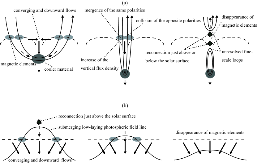
Figure 7: Schematic illustration for a flux cancellation without (panel a) and with (panel b) the observation of horizontal fields.

The subsurface advection of magnetic fields is as important as the surface advection for thinking about the observed motion of photospheric magnetic elements. In particular, if a subsurface field connects the opposite-polarity magnetic elements as a U-loop, our observations suggest the following interesting possibility. A cooler material sinking to the bottom of the U-loop would not only prevent the loop from rising, but may even force the loop to sink with the converging and downward convective flows, as sketched in Figure 7a. The cooler material can drag the subsurface field lines into a deeper layer via a downward convective flow because the plasma-$\beta$ is higher than unity below the photosphere, except for the strong magnetic fields associated with sunspots. This is similar to the idea of downward flux pumping by the turbulent granular convection around sunspots (Thomas et al., 2002). As a result of the forced submergence of the subsurface U-loop connecting the opposite polarity elements, these magnetic elements are driven by their Lorentz force to move toward the area with the large downward motion and then collide with each other (the middle panel of Fig. 7a). More detailed behaviors of flux tubes with the submergence of the subsurface U-loop can be found in Appendix A. Such a process is effective not only for the collision of the opposite polarities but also for the merging of the same polarities that are observed before the cancellation. Magnetic reconnection just above or below the solar surface would be needed for the disappearance of the colliding opposite polarity magnetic elements from the photosphere (the right panel of Fig. 7a), because the bottom of the subsurface field lines dragged by the downdrafts of cooler materials does not easily emerge into the photosphere. The reconnection site is still unknown from our observations, but the unresolved fine-scale flux removal process at such a site suggests magnetic reconnection, if any, is close to the photospheric surface. We of course have no observational evidence that a subsurface U-loop connects the opposite-polarity elements. Nevertheless, the events observed in this study can be explained by such a subsurface process.

4.2 Cancellation with Appearance of Horizontal Fields

The horizontal magnetic fields between the canceling opposite polarity elements have been observed along the intergranular lanes characterized with Doppler red shifts. The horizontal fields with the red shifts at the cancellation sites are already reported by Chae et al. (2004); Cheung et al. (2008); Iida et al. (2010). This cancellation is most probably a result of the submergence (retraction) of low-lying photospheric field lines along the intergranular lanes (Fig. 7b). Such low-lying photospheric field lines probably are formed by magnetic reconnection in the photosphere (or the bottom of the chromosphere) or by a failure of the emergence into the upper atmosphere. Recent three-dimensional (3D) radiative MHD simulations show the granular-scale flux cancellation due to a retraction of the $\Omega$-loop within an emerging flux region (Cheung et al., 2008). In the previous studies, the flux cancellations with the horizontal fields are reported in the moat region (Chae et al., 2004), within the emerging flux region (Cheung et al., 2008), or around the center of complicated active regions (Kubo & Shimizu, 2007). These regions basically contain many horizontal fields even if the horizontal field is not observed just before the cancellation. In our cancellation event with the horizontal field, small flux emergence accompanied by the appearance of horizontal fields is also observed well before the start of the event. The observing products during the cancellation may depend on the magnetic field configuration already formed before the approaching and canceling process. On the other hand, the opposite polarity elements approach the region with the converging flows, the darker intensity, and the large red shifts as in the case of cancellations without the observation of the horizontal fields. Therefore, the converging and downward motions are also important to bring one magnetic polarity element to another polarity element in this event.

5 CONCLUSION

We have presented an observational study of flux cancellation events on the photosphere that are sufficiently resolved by the Hinode SOT to show that they are characterized by the absence of a horizontal field during the cancellation process. These events are interesting because in the usual idea of the submergence of a low-lying $\Omega$-loop or the buoyant rise of a U-loop, the appearance of a horizontal field is the observational signature of the loop top (or bottom) passing across the photosphere. Such flux cancellations appear to be more common than the cancellation with the appearance of the horizontal fields. Although the nature of the flux removal process at the cancellation site is an open question for cancellations without the appearance of the horizontal fields, our study shows that it takes place in local areas at scales less than the $\sim$200km resolution of the SOT and close to the solar surface. The distinction between the cancellations with and without the appearance of the horizontal fields might arise from whether the canceling opposite polarity elements have emerged into the photosphere as a pair or not. However, we have investigated only 5 events that have the size less than a few arcseconds just outside the moat region of a sunspot. We need to investigate what really determines the appearance of the horizontal fields between the canceling magnetic elements by using more events. In particular, the origin of the canceling magnetic elements and their surrounding magnetic field configuration (formation of pre-existing horizontal fields) may be important.

We have confirmed the converging and downward convective flows are essential for the approaching and canceling process of the opposite-polarity magnetic elements. The flux cancellations are observed at the intergranular junction characterized by the strong converging and downward flows. However, the approaching opposite-polarity elements seem not to always follow the surrounding surface flow patterns, at least in our observations. We are accustomed to thinking of the connectivities of the surface magnetic fields that we can observe in the solar atmosphere. Our observational study suggests that it is important to also consider the connectivities of the surface fields that occur below the photosphere. Lanes of downdrafts of cool fluids entraining magnetic fluxes that thread across these lanes below the photosphere must be a common occurrence. Such a process is a simple explanation for a pair of opposite-polarity elements to appear to seek each other on the photosphere. Information of subsurface convective flows would be extremely helpful for better understanding of the magnetic flux cancellation.

Appendix A Discrete Magnetostatic Flux Tubes

The dynamical process sketched in Figure 7 is due to an interplay among pressure, gravitational and Lorentz forces in the neighborhood of a subphotospheric convective downflow. A proper study of this 3D time-dependent process requires numerical MHD simulation. On the other hand, some physical insight into that interplay can be seen in 3D static solutions of discrete magnetic flux tubes in a stratified atmosphere. Generally, such static solutions also require numerical computation but the family of analytical solutions taken from Low (1982) serves our purpose here.

Consider the magnetostatic equilibrium equations:

$${1\over 4\pi}\left(\nabla\times{\bf B}\right)\times{\bf B}-\nabla p-\rho g{\hat{z}}=0,$$ (A1)

$$\nabla\cdot{\bf B}=0,$$ (A2)

$$p=\rho{kT_{0}\over m},$$ (A3)

describing the force balance for a magnetic field ${\bf B}$ in an isothermal atmosphere at temperature $T_{0}$ and stratified by a uniform gravity with acceleration $g$ the $-z$-direction, using Cartesian coordinates. We use the ideal gas law (A3) where $k$ and $m$ denote the Boltzmann constant and the mean molecular weight of the plasma.

A 3D particular solution of these equations can be constructed for a magnetic field of the form

$${\bf B} = F(\phi,x)\nabla\phi\times\nabla x,$$ (A4)

$$= F(\phi,x)\left(0,{\partial\phi\over\partial z},-{\partial\phi\over\partial y}\right),$$

where $F(\phi,x)$ is an arbitrary function of two variables and

$$\phi={2\over k_{0}}exp(-{1\over 2}k_{0}z)\sin\left({1\over 2}k_{0}y\right),$$ (A5)

for some constant $k_{0}$. Direct substitution of this field into the magnetostatic equations shows that the equilibrium pressure must take the form

$$p=\left(P_{0}-{1\over 8\pi}F^{2}(\phi,x)\right)exp(-k_{0}z),$$ (A6)

introducing a constant $P_{0}$ and identifying $k_{0}^{-1}=kT_{0}/mg$ as the hydrostatic scale height which is of the order of $300~{}km$ at the photosphere at a temperature of about $6000K$.

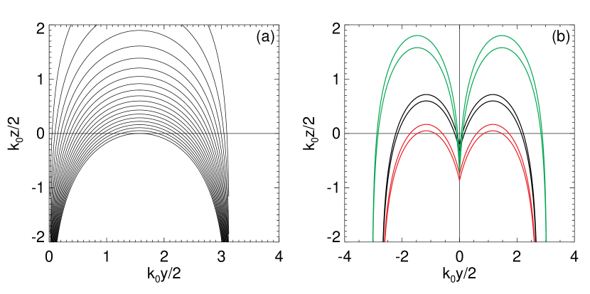
Figure 8: (a) Contours of constant $\phi(y,z)$, given by Eq.(A5), on a plane of constant $x$. (b) Three states of the M-shaped flux tube that is composed of two $\Omega$-shaped flux tubes joined at a kink.

This family of solutions is geometrically quite simple although it is three-dimensionally varying. Figure 8a shows the contours of constant $\phi(y,z)$ on a plane of constant $x$. The lines of force (LOFs) are all geometrically the same on each constant-$x$ plane but the field varies with all three Cartesian coordinates through its amplitude function $F(\phi,x)$ which is an arbitrary function to be prescribed. Take any explicit function $\sigma(\phi,x)$. Then, setting $\sigma=\sigma_{0}$, a constant, generates a magnetic flux surface in 3D space. To construct a flux tube of a finite cross section, a suitable functional form of $\sigma(\phi,x)$ set to a constant $\sigma_{0}$ describes a flux-tube boundary. Then, prescribing $F(\phi,x)\neq 0$ inside the tube and $F(\phi,x)\equiv 0$ in the rest of the atmosphere completes the construction. The atmospheric pressure distribution is then given by Equation (A6) which can also be expressed in the form

$$p+{B^{2}\over 8\pi}=P_{0}\exp(-k_{0}z).$$ (A7)

External to the flux tube, ${\bf B}=0$ so that $p=P_{0}\exp(-k_{0}z)$, the isothermal pressure of the field-free part of the atmosphere. Internal to the flux tube, the atmospheric pressure is reduced and compensated by the magnetic pressure so that the total pressure is stratified in the same manner as the external atmospheric pressure. This solution is mathematically analogous to the solution describing the equilibrium between a field ${\bf B}=B(x,y){\hat{z}}$ and fluid pressure in the absence of gravity. Equilibrium in this case is satisfied by requiring the total pressure $P=p+B^{2}/8\pi$ to be uniform in space. We have complete freedom to prescribe the field distribution and use this requirement to obtain the associated equilibrium pressure.

The static balance of forces may be viewed by writing Equation (A1) in the form

$${1\over 4\pi}\left({\bf B}\cdot\nabla\right){\bf B}-\nabla\left(p+B^{2}/8\pi\right)-\rho g{\hat{z}}=0,$$ (A8)

describing the balance among the forces of magnetic tension, total pressure, and gravity, represented by the three terms, respectively. Since the total pressure is vertically stratified everywhere, it follows that this class of equilibrium magnetic fields is characterized by a tension force that is vertically oriented everywhere (Low, 1984). Where the atmospheric plasma is threaded with a magnetic field, its pressure and density are reduced, so that this portion of the atmosphere is buoyant (Parker, 1979). The buoyancy force is just the net sum of the second and third terms in Equation (A8), and it is balanced by the remaining term which is the magnetic tension force. These solutions include linearly stable equilibrium states (Low, 1982).

To address the interplay among these magnetostatic forces, let us construct three equilibrium states, each corresponding to two $\Omega$-shaped flux tubes that are joined below the surface $z=0$ idealized to be the photosphere. These three states are displayed in Figure 8b shown as vertical sections of flux tubes boundary cut by a constant-$x$ plane. For each flux tube, its boundaries are drawn in different colors to identify them. Each pair of boundaries is the intersection of the flux-tube surface $\sigma=\sigma_{0}$ with the constant-$x$ plane.

Consider the M-shaped flux tube drawn in black, with boundaries $\phi(y,z)=0.4,0.45$. This flux tube is made up of two identically shaped tubes that join together below the origin where it is kinked. This flux tube intersects the photosphere $z=0$ at four places, giving two pairs of opposite-polarity magnetic elements on either sides of the origin. Since these elements are threaded by the same flux tube, the two elements on either side of the origin are of opposite polarities. The location of these two elements is controlled by the anchoring of the two parts of the flux tube at the kink below the origin. The infinitely long far arms are free to equilibrate with their surrounding fluid. The flux tube is everywhere in equilibrium except at the kink where an upward Lorentz force is assumed to be balanced by some force representing the effect, for example, of the ram pressure in a downdraft. The kinked part of the flux tube has a vertical thickness of about $0.05k_{0}$.

Suppose we forcefully move this kinked part of the flux tube from its original depth at about $0.1k_{0}$ below $z=0$ to about $0.35k_{0}$, keeping the same flux distribution inside the tube and the same vertical thickness at the kink. The new equilibrium of the flux tube is shown in red. The entire flux tube has sunk with that downward displacement of the kinked part. The opposite-polarity elements on the two sides of the origin drift apart to seek their opposite elements further away from the origin. This behavior can be understood as follows. The flux tube in this case does not extend very high into the atmosphere. The tube footpoint separations are of the order of a hydrostatic scale height, and the curvature at the tops of the tube is strong enough to produce a tension force comparable to the pressure and buoyancy forces at the temperature of about $6000K$ for the photosphere. When the kinked part of the flux tube is submerged further, an immediate effect is to increase that magnetic curvature. This enhances the magnetic tension force over the buoyancy force, leading to the submerging displacement for the whole flux tube.

The flux tube in green shows a different behavior as the result of the buoyancy force. In this case, the kinked part of the flux tube in black is submerged with two effects. The submergence elongates the vertical thickness of the kinked part of the flux tube while the cross section of the tube becomes more narrow. This elongation may be produced by a downward displacement that is larger at the bottom than at the top of the kinked part of the tube. The three-dimensionality of our magnetostatic solution is essential. If the field does not vary in $x$, we would have a flux layer rather than a flux tube. The entire atmosphere lying above it is trapped and cannot fall through without breaking the layer with variation in $x$. In our case, we have a true flux tube with a finite cross-sectional area. This means that the atmosphere external to the flux tube can yield and flow around a rising flux tube, for example. Moreover, the narrowing of the cross section of the tube enhances the magnetic pressure in the tube, which naturally produces a siphon flow along the flux tube to drain fluid down the far arms of the tube (Pikel’Ner, 1971; Thomas, 1988). The reduced weight of the tops of the tube becomes more buoyant and rise to a greater height. This brings about equilibrium with the external atmospheric pressure and a final balance between buoyancy and magnetic tension forces. The dynamical process builds up stress that pushes the two far arms away from the origin while at the same time brings the two opposite-polarity elements on either sides of the origin closer together, in a manner similar to the Hinode observations reported in this paper. In our Hinode observations the canceling opposite-polarity elements have fields that return to the photosphere at distances much larger than 10 hydrostatic scale heights from the canceling sites. We expect the buoyancy force to dominate in the atmospheric portion of the field, keeping the tops of these fields up in the chromosphere and above.

This simple theoretical analysis illustrates the interplay among the magnetic and hydrodynamic forces in the submergence of a field connection that happens to be located right at a subphotospheric convective downdraft. We of course need 3D time-dependent MHD simulations to examine the dynamics of this process to get a complete physical picture.

Figure 4: Stokes profiles of the Fe I 630.2 nm line at the pixels represented by squares in panel a of Fig. 3. The profiles in panels a-c are taken at 09:39:39, 09:45:02, and 09:50:30 on 2009 March 2, respectively. These profiles are normalized by the continuum intensity averaged over the quiet area. The vertical dashed line represents the averaged position of the line centers over the map.

References

- Bellot Rubio (2009) Bellot Rubio, L. R. 2009, ApJ, 700, 284
- Bellot Rubio & Beck (2005) Bellot Rubio, L. R., & Beck, C. 2005, ApJ, 626, L125
- Chae et al. (2004) Chae, J., Moon, Y., & Pevtsov, A. A. 2004, ApJ, 602, L65
- Cheung et al. (2008) Cheung, M. C. M., Schüssler, M., Tarbell, T. D., & Title, A. M. 2008, ApJ, 687, 1373
- de Wijn et al. (2008) de Wijn, A. G., Lites, B. W., Berger, T. E., Frank, Z. A., Tarbell, T. D., & Ishikawa, R. 2008, ApJ, 684, 1469
- Hagenaar (2001) Hagenaar, H. J. 2001, ApJ, 555, 448
- Harvey et al. (1999) Harvey, K. L., Jones, H. P., Schrijver, C. J., & Penn, M. J. 1999, Sol. Phys., 190, 35
- Iida et al. (2010) Iida, Y., Yokoyama, T., & Ichimoto, K. 2010, ApJ, in press
- Ishikawa & Tsuneta (2009) Ishikawa, R., & Tsuneta, S. 2009, A&A, 495, 607
- Jefferies et al. (1989) Jefferies, J., Lites, B. W., & Skumanich, A. 1989, ApJ, 343, 920
- Kosugi et al. (2007) Kosugi, T., et al. 2007, Sol. Phys., 243, 3
- Kubo et al. (2008) Kubo, M., Lites, B. W., Shimizu, T., & Ichimoto, K. 2008, ApJ, 686, 1447
- Kubo & Shimizu (2007) Kubo, M., & Shimizu, T. 2007, ApJ, 671, 990
- Lites et al. (2008) Lites, B. W., et al. 2008, ApJ, 672, 1237
- Litvinenko (1999) Litvinenko, Y. E. 1999, ApJ, 515, 435
- Low (1982) Low, B. C. 1982, ApJ, 263, 952
- Low (1984) Low, B. C. 1984, ApJ, 277, 415
- Martin, Livi, & Wang (1985) Martin, S. F., Livi, S. H. B., & Wang, J. 1985, Australian Journal of Physics, 38, 929
- Nisenson et al. (2003) Nisenson, P., van Ballegooijen, A. A., de Wijn, A. G., & Sütterlin, P. 2003, ApJ, 587, 458
- November & Simon (1988) November, L. J. & Simon, G. W. 1988, ApJ, 333, 427
- Orozco Suárez et al. (2007) Orozco Suárez, D., et al. 2007, PASJ, 59, 837
- Parker (1975) Parker, E. N. 1975, ApJ, 201, 494
- Parker (1979) Parker, E. N. 1979, Oxford, Clarendon Press; New York, Oxford University Press, 1979, 858 p.,
- Pikel’Ner (1971) Pikel’Ner, S. B. 1971, Sol. Phys., 17, 44
- Ryutova et al. (2003) Ryutova, M., Tarbell, T. D., & Shine, R. 2003, Sol. Phys., 213, 231
- Schrijver et al. (1997) Schrijver, C. J., Title, A. M., van Ballegooijen, A. A., Hagenaar, H. J., & Shine, R. A. 1997, ApJ, 487, 424
- Shimizu et al. (2008) Shimizu, T., et al. 2008, Sol. Phys., 249, 221
- Stenflo (1989) Stenflo, J. O. 1989, A&A Rev., 1, 3
- Takeuchi & Shibata (2001) Takeuchi, A., & Shibata, K. 2001, ApJ, 546, L73
- Thomas (1988) Thomas, J. H. 1988, ApJ, 333, 407
- Thomas et al. (2002) Thomas, J. H., Weiss, N. O., Tobias, S. M., & Brummell, N. H. 2002, Nature, 420, 390
- Tsuneta et al. (2008) Tsuneta, S., et al. 2008, Sol. Phys., 249, 167
- Yurchyshyn & Wang (2001) Yurchyshyn, V. B. & Wang, H. 2001, Sol. Phys., 202, 309
- Zwaan (1987) Zwaan, C. 1987, ARA&A, 25, 83