Density-matrix functionals for pairing in mesoscopic superconductors

Abstract

A functional theory based on single-particle occupation numbers is developed for pairing. This functional, that generalizes the BCS approach, directly incorporates corrections due to particle number conservation. The functional is benchmarked with the pairing Hamiltonian and reproduces perfectly the energy for any particle number and coupling.

While the Bardeen-Cooper-Schrieffer (BCS) microscopic theory Bar57 provides a suitable description of superconductivity in the macroscopic limit, it is not accurate enough for mesoscopic systems, such as nuclei, atomic clusters, quantum dots, fullerenes, nanotubes, or ultrasmall metallic grains Rin80 ; Von01 ; Bri05 ; Leg07 . Standard BCS approach to superconductivity has some drawbacks: (i) non negligible corrections due to finite size effects are necessary in mesoscopic systems; (ii) in condensed-matter and/or nuclear physics, BCS theory starting from the bare many-body interaction cannot be considered either as a numerically tractable approach nor as a predictive theory. To overcome difficulty (ii), specific functional theories based not only on the local density $\rho(r)$ but also on the anomalous density $\kappa(r,r^{\prime})$ are used Lud05 ; Ben03 . Guided by the Hamiltonian case, the energy is decomposed as:

$${\cal E}[\rho,\kappa] = {\cal E}[\rho]+{\cal E}_{\rm Pair}[\kappa,\kappa^{*}],$$ (1)

where ${\cal E}[\rho]$ is often taken as the energy density functional without pairing, while ${\cal E}_{\rm Pair}[\kappa,\kappa^{*}]$ is the extra contribution due to pairing. Eq. (1) turns out to be very accurate to deal with (ii) for instance in nuclear physics. In that case, systems with 10-200 constituents are considered and additional finite size corrections are necessary Rin80 ; Bla86 ; Bri05 . However, recent studies have shown that techniques generally used to restore good particle number should be handled with care when combined with density functional theories Dob07 ; Lac09 ; Ben09 ; Dug10 ; Rob10 . In particular, unless new methods able to properly treat finite size effects and more generally configuration mixing within functional theory, most of the functional designed during the last 30 years have to be revisitedDug09 . These difficulties question the possibility to use symmetry breaking within a functional theory.

The goal of the present work is to provide a new theoretical framework for pairing in finite systems that avoids difficulties recently encountered in functional theories and that can be applied easily be implemented in current functionals. Here, we follow the idea of GilbertGil75 ; Pap07 ; Lac09b and seek for a functional of occupation probabilities $n_{i}$ and natural orbitals $\varphi_{i}$, i.e. ${\cal E}\equiv{\cal E}[n_{i},\varphi_{i}]$. Note in passing, that (1) already enters into the class of Gilbert functionals. Indeed, the pairing energy is generally written as ${\cal E}_{\rm Pair}[\kappa,\kappa^{*}]=\sum_{ij}\bar{v}^{\kappa\kappa}_{ijkl}\kappa_{ij}\kappa^{*}_{kl}$ where $\bar{v}^{\kappa\kappa}$ denotes the effective two-body kernels in the particle-particle and hole-hole channels. In practice, both $\rho$ and $\kappa$ are computed using a quasi-particle (QP) vacuum trial state that can be seen as a generalization of the Kohn-Sham Slater determinant. If the energy is minimized in the canonical basis, the trial state, denoted by $|\phi\rangle$, takes a BCS like form $|\phi[n_{i},\varphi_{i}]\rangle=\prod_{i}\left(1+x_{i}a^{\dagger}_{i}a^{\dagger}_{\bar{i}}\right)|0\rangle$ with $x_{i}=\sqrt{n_{i}/(1-n_{i})}$ and where $|0\rangle$ corresponds to the particle vacuum while $\{a^{\dagger}_{i},a^{\dagger}_{\bar{i}}\}$ are associated to doubly degenerated canonical states $\{\varphi_{i},\varphi_{\bar{i}}\}$ with occupation probabilities $n_{i}$. In the canonical basis, $\kappa$ becomes block diagonal with $\kappa_{i\bar{i}}=\sqrt{n_{i}(1-n_{i})}$ and finally leads to an energy functional of the BCS occupation numbers. Functional based on BCS suffers for instance from the absence of pairing at weak coupling, it also misses part of the pairing effects at strong coupling (see for instance Pap07 ). These defects can be cured by considering many-body trial states projected onto good particle number. In that case, a reference QP state is first introduced, onto which the projection is made. The resulting energy becomes a rather complicated functional of the reference state She00 . However, serious difficulties appear when projection technique made before or after variation is combined with functional theories Dob07 ; Lac09 ; Ben09 ; Dug09 ; Rob10 .

Here, we use a completely different strategy and consider the projected state directly as the trial state. This state, called hereafter, Projected BCS state is written in its canonical basis as:

$$|N\rangle \equiv \frac{1}{\sqrt{N!}}(\Gamma^{\dagger})^{N}|-\rangle,$$ (2)

where $\Gamma^{\dagger}=\sum_{i}x_{i}b^{\dagger}_{i}$ with $b^{\dagger}_{i}=a^{\dagger}_{i}a^{\dagger}_{\bar{i}}$. $N$ denotes here the number of pairs. From this state, we define the occupation number and two-body correlation matrix elements through:

$$n_{i} \equiv \frac{\langle N|a^{\dagger}_{i}a_{i}|N\rangle}{\langle N|N\rangle},~{}~{}R_{ij}\equiv\frac{\langle N|b^{\dagger}_{i}b_{j}|N\rangle}{\langle N|N\rangle}.$$ (3)

Guided by the Hamiltonian framework, we propose to generalize the pairing energy and writes

$${\cal E}_{\rm Pair}[R,\varphi_{i}] = \sum_{ij}\bar{v}^{\kappa\kappa}_{i\bar{i}j\bar{j}}R_{ij}.$$ (4)

where $v^{\kappa\kappa}$ can eventually depend on the density of the projected state. By doing so, difficulties observed with projection are avoided. The main result of the present paper is to show that the correlation can be accurately written as a functional of occupation numbers of the projected state and account for finite size correction.

According to the definitions (3), both $n_{i}$ and $R_{ij}$ can be written as functionals of the parameter set $\{x_{i}\}$:

$$\left\{\begin{array}[]{lll}n_{i}&=&\displaystyle N|x_{i}|^{2}\frac{I_{N-1}(i)}{I_{N}},\\ R_{ij}&=&\displaystyle Nx^{*}_{i}x_{j}\frac{I_{N-1}(i,j)}{I_{N}}~{}~{}{\rm for}~{}~{}(i\neq j),\\ \end{array}\right.$$ (7)

while for $i=j$, $R_{ij}=\displaystyle n_{i}$. In these expressions, the following quantities have been defined (for any K such that $1<K\leq N$ and any $n$ with $n<\Omega$):

$$I_{K}(i_{1},\cdots,i_{n}) = \displaystyle\sum^{\neq}_{(j_{1},\cdots j_{K})\neq(i_{1},\cdots,i_{n})}|x_{j_{1}}|^{2}\cdots|x_{j_{K}}|^{2},$$ (8)

where $\sum^{\neq}$ means that the summation is made over all $(j_{1},\cdots j_{K})$ different from each other while $(j_{1},\cdots j_{K})\neq(i_{1},\cdots,i_{n})$ adds the constraint that all $j_{n}$ are different from $(i_{1},\cdots,i_{n})$. From the above discussion and as can be intuitively from the expression of the trial state (2), the energy can be written as an explicit functional of the $\{x_{i}\}$. Unfortunately, the complexity of this functional prohibits its use. A second difficulty of using $\{x_{i}\}$ as variational parameters is that they are not easily connected to quantities like occupation numbers adding complexity in physical interpretation. The BCS example illustrates that the energy can directly be written as a functional of the $\{n_{i}\}$ but is insufficient to precisely grasp the physics of pairing in finite systems.

Despite the complex relations between the occupation numbers and the $\{x_{i}\}$ (Eq. (7)), it is shown below that (i) the $\{x_{i}\}$ can be accurately replaced by a functional of the $\{n_{i}\}$; (ii) using this functional, the energy itself becomes a functional of the occupation probability only, that provides a very accurate description of the pairing Hamiltonian energy. Different relations given below are directly derived from recurrence relations existing for the $I_{K}$Van86 ; San08 ; Lac10 after tedious but straightforward calculations. We only give here main results are summarized here while technical details will be given elsewhere Lac10 .

Eqs. (7) can be rewritten as

$$n_{i} = \frac{|x_{i}|^{2}}{|x_{i}|^{2}+\alpha_{i}},~{}R_{ij}=\frac{x^{*}_{i}x_{j}}{|x_{i}|^{2}-|x_{j}|^{2}}(n_{i}-n_{j}),$$ (9)

where $\alpha_{i}\equiv I_{N}(i)/(NI_{N-1}(i))$.

An interesting connection with the BCS theory can be made by inverting the first expression in (9) as

$$|x_{i}|^{2} = \left(\frac{n_{i}}{1-n_{i}}\right)\alpha_{i}.$$ (10)

Reporting in the second equation of (9), leads to

$$R_{ij} = \sqrt{n_{i}(1-n_{i})n_{j}(1-n_{j})\alpha_{i}\alpha_{j}}$$ (11)

$$\times\frac{n_{i}-n_{j}}{n_{i}(1-n_{j})\alpha_{i}-n_{j}(1-n_{i})\alpha_{j}}.$$

Assuming $\alpha_{i}=\alpha_{j}=1$, this expression identifies with the BCS limit. Therefore, the physics associated with particle number restoration is all contained in the set of $\{\alpha_{i}\}$ parameters. The $\alpha$ parameters can be written as a function of the occupation numbers by performing a $(1/N)$ expansion assuming that the leading order identifies with the BCS limit one obtains Lac10 :

$$\alpha_{i} = 1-\frac{1}{N}n_{i}$$ (12)

$$+ \frac{1}{N(N-1)}\sum_{j\neq i}n_{j}^{2}[1-(n_{i}+n_{j})]$$

$$+ \frac{1}{N(N-1)(N-2)}\sum_{(k,j)\neq i}^{\neq}n_{j}^{2}n^{2}_{k}\left[2-(n_{i}+n_{j}+n_{k})\right]$$

$$+ \cdots$$

which is nothing but $\alpha_{i}$ written as an explicit functional of the occupation numbers. By replacing $\alpha_{i}$ given above in $R$ and then the expression of $R$ in (4), the energy become an explicit functional of the occupation numbers through the sequence

$${\cal E}[\rho,R,\varphi_{i}] \rightarrow {\cal E}[\{x_{i}\},\varphi_{i}]\rightarrow{\cal E}[\{n_{i}\},\varphi_{i}].$$ (13)

In practice, the new expression we obtained for ${\cal E}$ can directly replace the BCS expression in theories either based on a Hamiltonian or directly formulated in a density functional framework. Since the functional is directly formulated in terms of natural orbitals and occupancies, one should add specific constraint during the minimization. Below, the quantity:

$${\cal E}^{\prime}[\{n_{i}\},\varphi_{i}] = {\cal E}[\{n_{i}\},\varphi_{i}]-\mu\left(\sum n_{i}-N\right),$$ (14)

is directly minimized.

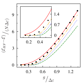
Figure 1: (Color online) Difference between the Hartree-Fock energy ${\cal E}_{HF}$ and the exact Richardson solution (red solid line) of ref. San08 , generally referred as the condensation energy, compared to result obtained with successive approximation using expression (12) for 8 particles. The dashed, dotted, dot-dashed lines and filled circles correspond respectively to the BCS, first, second and third order correction. In insert, a focus on the weak coupling region is shown. Note that the PBCS energy (not shown here) cannot be distinguished from the exact result.

In order to test the functionals developed here, we consider an even system of A particles interacting through the ”picket” fence Hamiltonian of the form Ric64

$$H=\sum_{i}\varepsilon_{i}(a^{\dagger}_{i}a_{i}+a^{\dagger}_{\bar{i}}a_{\bar{i}})-g\sum_{i,j}a^{\dagger}_{i}a^{\dagger}_{\bar{i}}a_{\bar{j}}a_{j},$$ (15)

with doubly degenerate equidistant levels and with a level spacing $\Delta\varepsilon$. In the following, $N=A/2$ denotes the number of pairs while $\Omega=4N$ is the single-particle space size. For this Hamiltonian, the energy simply writes ${\cal E}(n_{i},R_{ij})\equiv 2\sum_{i}\varepsilon_{i}n_{i}-g\sum_{ij}R_{ij}$. Note that, this functional interaction corresponds to (4) with $v^{\rho\rho}_{i\bar{i}j\bar{j}}=v^{\kappa\kappa}_{i\bar{i}j\bar{j}}=g$. The pairing Hamiltonian can be solved exactly and therefore is particularly suitable for benchmarking approximation for pairing correlationVon01 ; Duk04 .

An illustration of successive corrections beyond the BCS approximation is given in figure 1. Results are obtained using the functional form of $R$ where $\alpha_{i}$ are replaced by Eq. (12) trunctated at a given order. Then, Eq. (14) is directly minimized starting from the BCS solution and making variation of occupation numbers between 0 and 1. A quadratic programming (QP) method is used for the minimization leading to rapid convergence tested up to 400 particles. Systematic improvement is observed as higher orders in the correction are included. The above functional has however two major drawbacks. First, it is rather complicated to use. Second, while few terms are necessary to get a perfect result in the strong coupling, the convergence is rather slow in the weak coupling regime. It could indeed be shown that all terms in the expansion up to order $1/N!$ contribute equally in the Hartree-Fock limit. This directly stems from the inadequacy of the BCS functional in the weak coupling limit. For instance, a direct use of perturbation theory leads to much better results underlying the role of $2$ particles-$2$ holes excitations (see for instance discussion in San08 ).

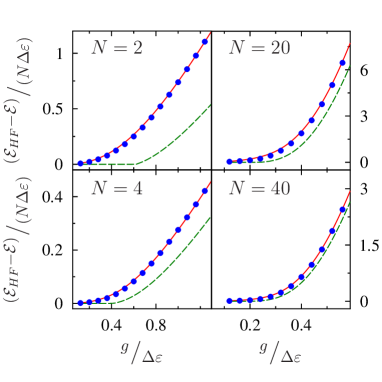
Figure 2: (Color online) Comparison between the exact condensation energy (solid line), the BCS (dashed line) and the result obtained by minimizing the density matrix functional (filled circles) with the approximation (17) for various particle numbers and coupling strength . Again in all cases, the PBCS result is in perfect agreement with the exact one.

This difficulty could only be overcome by considering these terms explicitly, which in the form given by (12) becomes impractical for numerical implementation as $N$ increases. A simple linear expression, i.e.

$$\alpha_{i}=a_{0}+a_{1}n_{i},$$ (16)

can however be found by considering all terms in the expansion and approximating sums in (12) according to:

$$\frac{1}{N(N-1)}\sum_{j\neq i}\rightarrow\frac{1}{N^{2}}\sum_{j},$$

$$\frac{1}{N(N-1)(N-2)}\sum_{(k,j)\neq i}^{\neq}\rightarrow\frac{1}{N^{3}}\sum_{jk},\cdots$$

A straightforward calculation then gives:

$$a_{1} = -\frac{1}{N}\frac{1-s_{2}^{N}}{1-s_{2}},~{}~{}a_{0}=1-(s_{2}-s_{3})\frac{\partial a_{1}}{\partial s_{2}},$$ (17)

where $s_{p}=\frac{1}{N}\sum_{i}(n_{i})^{p}$. Note that, due to the re-summation of expansion (12) of all terms up to order $N$, the present approach could not be anymore regarded as a $1/N$ correction. Energies obtained with this approximation are shown in figure 2 for various particle numbers and couplings. The energy found by minimizing the functional is overall in very good agreement with the exact energy for any particle number and coupling.

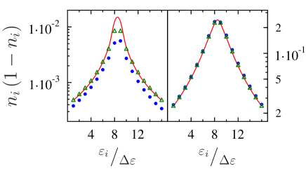
Figure 3: (Color online) Evolution of $n_{i}(1-n_{i})$ as a function of $\varepsilon_{i}/\Delta\varepsilon$ for the exact (solid line), PBCS (open triangles), and the new functional (filled circles) for $A=16$ and $g/\Delta\varepsilon=0.16$ (left) and $0.56$ (right).

A careful analysis shows a slight underestimation of the energy in the intermediate coupling regime associated also with a slight difference in the occupation numbers (see figure 3). This small discrepancy stems from the linear approximation made for the $\alpha_{i}$. To better account for occupation number behavior, quadratic or cubic corrections to (16) might eventually be obtained. However, this will add complexity to the functional while the energy is already rather well reproduced.

In this letter, a new approach is proposed to account for pairing in finite systems using functional theories. To escape difficulties recently observed Dob07 ; Lac09 ; Ben09 ; Dug09 , namely divergences and jumps, the introduction of an auxiliary QP state is avoided and a Projected BCS trial state is directly used. In the pairing hamiltonian, a perfect agreement between the functional result and the exact energy is obtained at all coupling strength and particle number. The present method can be directly implemented on existing functional theories and should provide an accurate way to treat finite size effects. Note that present approach can easily be extended to odd systems Lac10 and might provide a tool of choice to study dynamics and thermodynamics of finite systems with pairing. Guided by the BCS theory, system at finite temperature can be studied minimizing the free energy defined through :

$${\cal F}[\{n_{i}\},\varphi_{i}]={\cal E}^{\prime}[\{n_{i}\},\varphi_{i}]-T{\cal S}[n_{i}].$$ (18)

Note that, the present theory has been recently applied to nuclei showing that it solves recent difficulties associated to broken symmetries Dob07 ; Lac09 opening new perspectives.

- (1) J. Bardeen, L. N. Cooper, and J. R. Schrieffer, Phys. Rev. 106, 162 (1957); Phys. Rev. 108, 1175 (1957).
- (2) P. Ring and P. Schuck, The Nuclear Many-Body Problem (Springer Verlag, 1980).
- (3) J. von Delft and D.C. Ralf, Phys. Rep. 345, 61 (2001). F. Braun, J. von Delft, Phys. Rev. Lett. 81, 21 (1998).
- (4) D.M. Brink and R.A. Broglia, Nuclear superfluidity: pairing in finite systems, (Cambridge Univ. Press, 2005).
- (5) A.J. Leggett, ”Quantum liquids and cooper pairing in condensed-matter systems”, Oxford University Press, (2006).
- (6) M. Bender, P.-H. Heenen, and P.-G. Reinhard Rev. Mod. Phys. 75, 121 (2003).
- (7) M. Lüders et al, Phys. Rev. B72, 024545 (2005).
- (8) J.-P. Blaizot and G. Ripka, Quantum Theory of Finite Systems (MIT Press, 1986).
- (9) J. Dobaczewski, M. Stoitsov, W. Nazarewicz, and P.-G. Reinhard, Phys. Rev. C 76, 054315 (2007).
- (10) D. Lacroix, T. Duguet, and M. Bender, Phys. Rev. C 79, 044318 (2009).
- (11) M. Bender, T. Duguet, and D. Lacroix, Phys. Rev. C 79, 044319 (2009).
- (12) T. Duguet and J. Sadoudi, preprint arXiv:1001.0673.
- (13) L. M. Robledo, preprint arxiv:1003.3043.
- (14) T. Duguet, M. Bender, K. Bennaceur, D. Lacroix, and T. Lesinski Phys. Rev. C 79, 044320 (2009).
- (15) T. L. Gilbert, Phys. Rev. B 12, 2111 (1975).
- (16) D. Lacroix, Phys. Rev. C 79, 014301 (2009).
- (17) T. Papenbrock and A. Bhattacharyya, Phys. Rev. C 75, 014304 (2007).
- (18) J. A. Sheikh and P. Ring, Nucl. Phys. A665, 71 (2000).
- (19) N. Sandulescu and G.F. Bertsch, Phys. Rev. C 78, 064318 (2008). N. Sandulescu, B. Errea, and J. Dukelsky Phys. Rev. C 80, 044335 (2009).
- (20) P. Van Isacker, S. Pittel, A. Frank and P.D. Duval, Nucl. Phys. A451, 202 (1986).
- (21) G. Hupin and D. Lacroix, in preparation.
- (22) R. W. Richardson and N. Sherman, Nucl. Phys. 52, 221 (1964). R. W. Richardson, Phys. Rev. 141, 949 (1966). R. W. Richardson, J. Math. Phys. 9, 1327 (1968).
- (23) J. Dukelsky, S. Pittel, and G. Sierra, Rev. Mod. Phys. 76, 643 (2004).
- (24) R. Balian, Am. J. Phys. 67, 1078 (1999).