Diffusion-Limited Aggregation on Curved Surfaces

Abstract

We develop a general theory of transport-limited aggregation phenomena occurring on curved surfaces, based on stochastic iterated conformal maps and conformal projections to the complex plane. To illustrate the theory, we use stereographic projections to simulate diffusion-limited-aggregation (DLA) on surfaces of constant Gaussian curvature, including the sphere ($K>0$) and pseudo-sphere ($K<0$), which approximate “bumps” and “saddles” in smooth surfaces, respectively. Although curvature affects the global morphology of the aggregates, the fractal dimension (in the curved metric) is remarkably insensitive to curvature, as long as the particle size is much smaller than the radius of curvature. We conjecture that all aggregates grown by conformally invariant transport on curved surfaces have the same fractal dimension as DLA in the plane. Our simulations suggest, however, that the multifractal dimensions increase from hyperbolic ($K<0$) to elliptic ($K>0$) geometry, which we attribute to curvature-dependent screening of tip branching.

The Laplacian growth model and its stochastic analogue, diffusion-limited aggregation (DLA) witten81 , describe the essential physics of non-equilibrium pattern formation in diverse situations bunde , such as viscous fingering bensimon86 , (quasi-static) dendrite solidification kessler88 , dielectric breakdown niemeyer84 , and dissolution TLD , depending on conditions at the moving, free boundary. Some extensions to non-Laplacian growth phenomena, such as advection-diffusion-limited aggregation adla ; david05 (ADLA) and brittle fracture barra02 , are also available. Almost all prior work with these models has assumed flat Euclidean space, typically a two-dimensional plane, but real aggregates, such as mineral dendrites chopard91 , cell colonies wang97 , and cancerous tumors ho98 , often grow on curved or rough surfaces. Aside from a few studies of Eden-like clusters wang97 and continuous viscous fingers entov97 ; parisio01 on spheres, it seems that the effects of surface curvature on pattern formation have not been investigated.

In this Letter, we extend transport-limited growth models to curved two-dimensional surfaces via conformal projections from the plane. Time-dependent conformal maps are widely used in physics gruzberg04 and materials science handbook to describe interfacial dynamics in two dimensions. Continuous conformal maps have long been applied to viscous fingering howison92 ; bensimon86 , and more recently, Hastings and Levitov introduced stochastic, iterated conformal maps for DLA hastings98 . Both continuous and stochastic conformal-map dynamics have also been extended to other conformally invariant (but non-Laplacian and nonlinear) gradient-driven transport processes bazant04 ; adla ; david05 , such as advection-diffusion in a potential flow kornev94 ; choi05 or electrochemical transport in a quasi-neutral solution bazant04 . Indeed, there is nothing special about harmonic functions (solutions to Laplace’s equation) in the plane, aside from the direct connection to analytic functions of a complex variable (real or imaginary part). The key property of conformal invariance is shared by other equations bazant04 ; handbook and, as note here, applies equally well to conformal (i.e. angle preserving) transformations between curved surfaces. Here, we formulate continuous and discrete conformal-map dynamics for surfaces of constant curvature, by a sequence of mappings from the complex plane, and we use the approach to study the fractal and multi-fractal properties of DLA on curved surfaces.

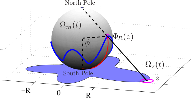
Figure 1: Stereographic projection, $\Phi^{-1}$, from the exterior of the growing object $\Omega_{m}(t)$ on a sphere of radius $R$ to the exterior of the shadow, $\Omega_{z}(t)$, on a complex plane. The point $\Phi(z)$ is projected from the north pole to the point $z$. The origin of the $z$-plane is tangent to the sphere at the south pole, and the latitudinal angle $\phi$ is measured from the south pole.

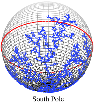
(a)   (b)

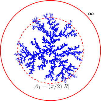
Figure 2: DLA clusters on the elliptic (left) and the hyperbolic (right) geometries. The elliptic geometry is isometrically embedded on the surface of a sphere and the hyperbolic geometry is visualized on the Poincaré disk with the metric, $ds=dz/(1-(|z|/2R)^{2})$. We use $R/\sqrt{\lambda_{o}}=100$ and aggregate 4942 and 9001 particles to fill the great circles of radius $(\pi/2)R$ (dashed lines) in the elliptic and hyperbolic geometries respectively.

Transport-limited growth on curved surfaces. — At first, it would seem that conformal-map dynamics cannot be directly applied to a non-Euclidean geometry, and certainly the formulation could not be based only upon analytic functions of the complex plane. Nevertheless, if there exists a conformal (angle-preserving) map between the curved manifold and the plane, and if the underlying transport process is conformally invariant bazant04 ; choi05 ; adla ; david05 ; handbook , then any solution to the transport equations in the non-Euclidean geometry can be conformally mapped to a solution in the complex plane, without changing its functional form. Such maps do exist, as we illustrate below with important special cases.

Let $\Omega_{m}(t)$ be the exterior of a growing object on a non-Euclidean manifold, $M$, and $\Phi$ be a conformal map from a (part of) complex plane to $M$. We speak of the domain $\Omega_{m}(t)$ as having its shadow, $\Omega_{z}(t)=\Phi^{-1}(\Omega_{m}(t))$, on the complex plane under the projection $\Phi^{-1}$. As in the flat surface case, we can describe the growth by a time-dependent conformal map, $g(w,t)$, from the exterior of the unit disk, $\Omega_{w}$, to the exterior of the growing shadow, $\Omega_{z}(t)$, which in turn is mapped onto the curved geometry by the inverse projection. Care must only be taken that the dynamics of $g(w,t)$ should describe $\Omega_{z}(t)$ in such a way that the evolving object, $\Omega_{m}(t)$, follows the correct physics of growth on $M$, rather than in the intermediate complex plane, which is purely a mathematical construct.

Let us illustrate this point for both continuous and discrete versions of conformally invariant, transport-limited growth adla ; handbook . For continuous growth, we generalize the Polubarinova-Galin equation equation polub45 ; adla ; handbook for a curved manifold with a conformal map $\Phi(z)$ as follows

$$\mathrm{Re}\,\{\overline{w\ g^{\prime}(w)}\ g_{t}(w)\}=\frac{\alpha\;\sigma(w,\,t)}{|\Phi^{\prime}\circ g(w)|^{2}}.$$ (1)

for $|w|=1$, where $\alpha$ is a constant and $\sigma(w,\,t)$ is the time-dependent flux density on the boundary of $\Omega_{w}$. This result is easily obtained by substituting $\Phi\circ g$ for $g$ in the original equation.

For stochastic growth, we adjust the Hastings-Levitov algorithm hastings98 on the shadow domain. The algorithm is based on the recursive updates of the map,

$$g_{n}(w)=g_{n-1}\circ\phi_{\lambda_{n},\theta_{n}}(w),\quad g_{n}(w)=g(w,t_{n}),$$ (2)

where $\phi_{\lambda,\theta}$ is a specific map that slightly distort $\Omega_{w}$ by a bump of area $\lambda$ around the angle $\theta$. While the random sequence $\{\theta_{n}\}$ follows the probability distribution, $p(\theta,t_{n})\propto\sigma(e^{i\theta},t_{n})$, invariant under conformal maps, the preimage of bump area, $\lambda_{n}$, should be determined so that the bump area is fixed as $\lambda_{0}$ on the manifold, $M$. Thus the bump size of the $n$-th accretion is determined by

$$\lambda_{n}=\frac{\lambda_{0}}{|\Phi^{\prime}\circ g_{n-1}(e^{i\theta_{n}})|^{2}\cdot|g_{n-1}^{\prime}(e^{i\theta_{n}})|^{2}}.$$ (3)

We are not aware of any prior modification of the Hastings-Levitov algorithm with this general form. Previous studies on DLA in a channel geometry somfai03a can be viewed as an example with $M=\{z:\;0<{\rm arg}\;z<2\pi\}$ and $\Phi(z)=\log(z)$ although the manifold is Euclidean.

Stereographic projections. To illustrate the general theory, we first make use of classical stereographic projection needham to describe growth on a sphere. Stereographic projection is obtained by projecting the surface of a sphere from the north pole to a plane whose origin is tangent to the south pole; see Fig. 1. If $\Phi$ is an inverse stereographic projection with sphere of radius $R$, $\Phi^{-1}$ maps the point $(R,\phi,\theta)$ in spherical coordinates to $z=R\tan(\phi/2)e^{i\theta}$ in the complex plane. Here $\theta$ is the azimuthal angle and $\phi$ is the latitudinal angle measured from the south pole. If the modulus, $|\,\cdot\,|$, on the sphere is defined to be distance to the origin (south pole) in the curved metric (arc-length of the great circle) in a similar way to $|\,\cdot\,|$ on a complex plane, $|z|$ and $|\Phi(z)|$ satisfy

$$\frac{|z|}{2R}=\tan\left(\frac{|\Phi(z)|}{2R}\right).$$ (4)

The Jacobian factor of the projection is angle-independent; thus, it is given by

$$|\Phi^{\prime}(z)|=\frac{d|\Phi(z)|}{d|z|}=\frac{1}{1+(|z|/2R)^{2}}$$ (5)

from the derivative of Eq. (4). Now Eq. (5) can be used to continuous dynamics, Eq. (1), and stochastic dynamics, Eq. (3) on sphere.

While the surface of a sphere is a three-dimensional visualization of elliptic (or Riemannian) geometry, we can also obtain a conformal projection from hyperbolic geometry to a complex plane as well. Unlike elliptic geometry, hyperbolic geometry can not be isometrically embedded into 3D Euclidean space; only a part of the geometry can be embedded into 3D as a surface known as pseudosphere. Hyperbolic geometry has a negative constant curvature, $K=-1/R^{2}$, as opposed to the positive one, $K=1/R^{2}$, of elliptic geometry. The projection can be obtained by simply viewing hyperbolic geometry as a surface of a sphere with an imaginary radius, $iR$, as suggested from the sign of curvature. The projection can be still defined; substituting $iR$ for $R$ alters Eqs. (4) and (5) as

$$\frac{|z|}{2R}=\tanh\left(\frac{|\Phi(z)|}{2R}\right)\qquad\text{and}\qquad|\Phi^{\prime}(z)|=\frac{1}{1-(|z|/2R)^{2}}.$$ (6)

The image of hyperbolic geometry under the projection is thus limited to the inside of a disk with radius $2R$, and the boundary, $|z|=2R$, corresponds to the infinity. The stereographic projection serves as a non-isometric visualization of the geometry known as Poincaré disk. The length element $dz$ at $dz$ in the disk corresponds to the element $dz/(1-(|z|/2R)^{2})$ in the hyperbolic universe.

Geometry	Elliptic	Euclidean	Hyperbolic
${D_{f}}$	1.704$\pm$0.001	1.704$\pm$0.001	1.693$\pm$0.001
$D_{2}/{D_{f}}$	0.577$\pm$0.003	0.529$\pm$0.006	0.527$\pm$0.001
$D_{3}/{D_{f}}$	0.591$\pm$0.006	0.503$\pm$0.005	0.499$\pm$0.001
$D_{4}/{D_{f}}$	0.617$\pm$0.012	0.486$\pm$0.004	0.482$\pm$0.001
$D_{5}/{D_{f}}$	0.631$\pm$0.018	0.473$\pm$0.004	0.469$\pm$0.001

Table 1: The fractal dimension ${D_{f}}$ and the multifractal dimensions $D_{2q+1}$ of DLA clusters on three different geometries.

(a)
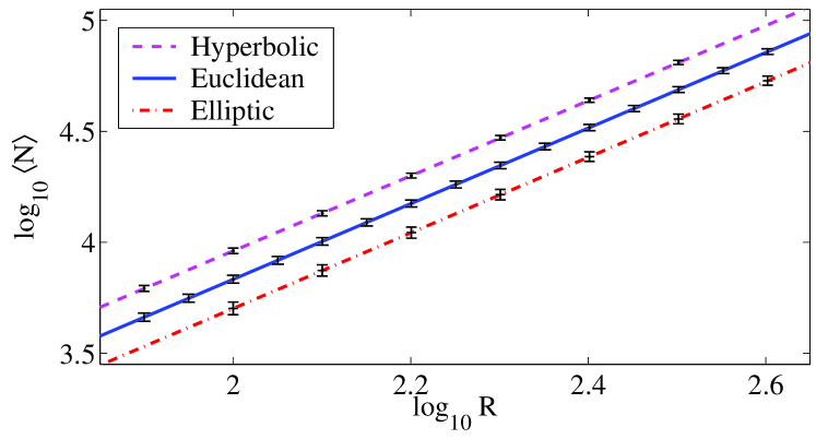
(b)

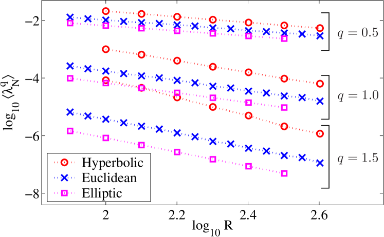
Figure 3: (a) The average number of particles, $\langle{N}\rangle$, to fill the disk of conformal radius, $\mathcal{A}_{1}=(\pi/2)R$, versus radius $R$ on the three geometries. (b) Moments $\langle{\lambda_{N}^{q}}\rangle$ of the pre-image bump size, $\lambda_{N}$, versus $R$, which define $D_{2q+1}$ via (9.

DLA on constant-curvature surfaces. — Using the harmonic probability measure, $p(\theta)=1/2\pi$, and the modified Hastings-Levitov algorithm with Eq. (3), we grow DLA clusters on curved surfaces. Fig. 2 shows clusters on elliptic and hyperbolic geometries. On the Poincaré disk, the size of particles becomes smaller and smaller as they approach the infinity, $|z|=2R$.

An analytic advantage of the conformal mapping formulation is that the Laurent expansion of $g(w,t)$ gives us information on the moments of the cluster; the conformal radius, $A_{1}$, and the center of charge, $A_{0}$, come from the first two terms of the expansion, $g(w)\approx A_{1}w+A_{0}$. Such coefficients from DLA clusters on curved surfaces are not useful as they are the moments of the shadow, not the original cluster. Using the property that circles are mapped to circles under an (inverse) stereographic projection, it is possible to define analogous quantities corresponding to $A_{1}$ and $A_{0}$. We note that the image, $\Phi(A_{1}w+A_{0})$, of the unit circle, $|w|=1$, is also a circle on $M$, and it is the one that best approximate the cluster and the far-field in $\Omega_{m}(t)$. Thus, we define the conformal radius, $\mathcal{A}_{1}$, and the center of charge, $\mathcal{A}_{0}$, on $M$ to be the radius and the deviation of $\Phi(A_{1}w+A_{0})$ respectively:

$$\mathcal{A}_{1}=\frac{1}{2}\;\{\;|\Phi(A_{1}+|A_{0}|)|+|\Phi(A_{1}-|A_{0}|)|\;\},$$ (7)

$$\mathcal{A}_{0}=\frac{1}{2}\;\{\;|\Phi(A_{1}+|A_{0}|)|-|\Phi(A_{1}-|A_{0}|)|\;\}.$$ (8)

On curved surfaces, however, the fractal dimension ${D_{f}}$, cannot be determined from the scaling, $n\sim\langle{\mathcal{A}_{1}}\rangle^{D_{f}}$, since the geometry is not linearly scalable with $\mathcal{A}_{1}$; the two domains within radii of different values of $\mathcal{A}_{1}$ are not self-similar to each other, and the log-log plot of $n$ versus $\mathcal{A}_{1}$ is not linear either. Instead, we use the sphere radius $R$ as a relevant length scale while keeping $\mathcal{A}_{1}$ proportional to $R$ for self-similarity. Thus, we grow a cluster until $\mathcal{A}_{1}$ reaches at $\phi_{o}R$ for various radius $R$, but with a fixed particle size, $\lambda_{o}=1$, and a fixed angle $\phi_{o}=\pi/2$. The angle $\phi_{o}$ is as such since the circle (dashed lines in Fig. 2) becomes a great circle on a sphere. If $N$ is the number of particles to fill the radius, the fractal dimension is determined from $\langle{N}\rangle\sim R^{{D_{f}}}$. From the statistics of 1000 clusters for each of $R$ in a geometrically increasing sequence from 79 to 400, we obtain the fractal dimensions, ${D_{f}}\approx 1.70$, as shown in Table 1. Fig. 3(a) shows $\langle{N}\rangle$ versus $R$ in the three geometries. The relative deviation of ${D_{f}}$ between geometries is surprisingly small compared to the deviation of surface properties caused by the curvature. For example, the area within the radius $(\pi/2)R$ on elliptic (or hyperbolic) geometry is about 23% smaller (or larger) than the corresponding area on the Euclidean surface; however, this factor only change the prefactor, not the exponent, of the scaling, $\langle{N}\rangle\sim R^{{D_{f}}}$.

Our results suggest that ${D_{f}}$ is insensitive to the curvature because, on small length scales comparable to the the particle size $\sqrt{\lambda_{0}}$, the surface is locally Euclidean. This result is consistent with ADLA adla ; david05 whose fractal dimension is not affected by the background fluid flow. We conjecture that any conformally invariant transport-limited aggregation process on a $d$-dimensional curved manifold has same, universal fractal dimension as DLA in flat (Euclidean) space in $d$ dimensions.

More subtle statistics of the aggregates, however, are revealed by multifractal scalings. The multifractal properties hentschel83 ; halsey86 related to from the probability measure, however, seem to depend on the curvature. Following Ref. david99 , we measure the multifractal dimensions $D_{q}$ from the relation,

$$\langle{\lambda_{N}^{q}}\rangle\sim R^{-2qD_{2q+1}}.$$ (9)

The averaging in Eq. (9) is made over $\lambda_{N}$ at uniformly distributed angle. Fig. 3(b) shows the first three moments of $\lambda_{N}$ as functions of $R$, and Table  1 shows $D_{q}/{D_{f}}$ in the three geometries. We note that $D_{q}$ for elliptic geometry are yet transient, influenced by finite-size effect. The multifractal dimensions do not satisfy the inequality $D_{q}>D_{q^{\prime}}$ for $q<q^{\prime}$ hentschel83 . Since the space itself is finite and the distance to infinity is bounded, the instability in growth is pronounced in elliptic geometry. The normalized center-of-charge fluctuation, $\langle{|\mathcal{A}_{0}|^{2}}\rangle^{1/2}/R$, is about 0.3 for on elliptic geometry although it decreases as $R$ increases. For Euclidean and hyperbolic geometries, the fluctuations are around 0.03 and 0.02 respectively. It should also be noted that the growth probability on sphere is not harmonic since the far-field potential, $-\log|z|$, on plane is mapped to the singular potential, $\log(\pi-\phi)$, around the north pole.

Even with the finite size effect, we conjecture that multifractal dimensions increase in the order of hyperbolic, Euclidean, and elliptic geometries. The justification is that, when the measurements are similarly made for smaller latitudinal angles, $\phi_{o}=\pi/3$ and $\pi/6$, $D_{q}$ on elliptic and hyperbolic geometries converge to $D_{q}$ on Euclidean plane. This also support that the slight difference in $D_{q}$ between Euclidean and hyperbolic geometries are not from statistical error. We believe the dependence of $D_{q}$ on curvature is related to the depth of fjords. On elliptic geometry, the circumference of a circle with radius $\phi_{o}R$ is $2\pi\sin\phi_{o}R$, shorter than $2\pi\phi_{o}R$ on Euclidean geometry. If we consider a pair of branches which make the same opening angle on the two geometries, the area between them is more screened on elliptic than on Euclidean geometry. Therefore, we expect a different distribution of $\lambda$. Due to the competition on smaller circumference, tip-splitting events are subdued, as observed in continuous growth parisio01 , and eventually fewer branches survive. The opposite argument applies to hyperbolic geometry, where the circumference is given by $2\pi\sinh\phi_{o}R$, inter-branch area is less-screened, and tip-splitting is encouraged. In future work, it would be interesting to analyze the spectrum of $\lambda$ and its connection to tip splitting events.

In summary, we have developed a mathematical theory of transport-limited growth on curved surfaces and applied it to DLA on two-dimensional surfaces of constant Gaussian curvature. Our simulations suggest that the fractal dimension of DLA clusters is universal, independent of curvature, and depends only on the spatial dimension. The multifractal properties of DLA, however, seem to depend on curvature, since tip-splitting is related to the different degrees of screening the inter-branch areas. We conjecture that these results are hold in general, for any conformally invariant transport-limited growth process, in any number of dimensions.

We acknowledge helpful discussions with Ellak Somfai.

References

- (1) I. Gruzberg and L. P. Kadanoff, J. Stat. Phys. 114, 1183 (2004).
- (2) A. Bunde and S. Havlin (eds.) Fractals and Disordered Systems, second edition (Springer, New York, 1996).
- (3) T. A. Witten and L. M. Sander Phys. Rev. Lett. 47, 1400 (1981).
- (4) D. Bensimon, L. Kadanoff, B. I. Shraiman, and C. Tang, Rev. Mod. Phys. 58, 977 (1986).
- (5) D. A. Kessler, J. Koplik and H. Levine, Adv. Phys. 37, 255 (1988).
- (6) L. Niemeyer, L. Pietronero, and H. J. Wiesmann, Phys. Rev. Lett. 52, 1033 (1984).
- (7) D. Bensimon, L. P. Kadanoff, S. Liang, B. I. Shraimain, and C. Tang, Rev. Mod. Phys. 58, 977 (1986).
- (8) S. D. Howsion, Eur. J. Appl. Math. 3, 209 (1992).
- (9) K. Kornev and G. Mukhamadullina, Proc. R. Soc. London, Ser. A 447, 281 (1994).
- (10) M. Z. Bazant, Proc. Roy. Soc. A. 460, 1433-1452 (2004).
- (11) J. Choi, D. Margetis, T. M. Squires, and M. Z. Bazant, J. Fluid Mech. 536, 155-184 (2005).
- (12) M. Z. Bazant, Phys. Rev. E 73, 060601 (2006).
- (13) F. Barra, A. Levermann and I. Procaccia, Phys. Rev. E 66, 066122 (2002).
- (14) B. Davidovitch, J. Choi, and M. Z. Bazant, Phys. Rev. Lett. 95, 075504 (2005).
- (15) M. Z. Bazant and D. Crowdy, in Handbook of Materials Modeling, ed. by S. Yip et al., Vol. I, Art. 4.10 (Springer, 2005).
- (16) P. Ya. Polubarinova-Kochina, Dokl. Akad. Nauk. S. S. S. R. 47, 254 (1945); L. A. Galin, 47, 246 (1945).
- (17) M. Z. Bazant, J. Choi, and B. Davidovitch, Phys. Rev. Lett. 91, 045503 (2003).
- (18) B. Chopard, H. J. Herrmann, and T. Vicsek, Nature 353, 409 (1991).
- (19) C. Y. Wang and J. B. Bassingthwaighte, Math. Biosci. 142, 91 (1997).
- (20) P. F. Ho and C. Y. Wang, Math. Biosci. 155, 139 (1999).
- (21) V. M. Entov and P. I. Etingof, Euro. J. of Appl. Math. 8, 23 (1997)
- (22) F. Parisio, F. Moraes, J. A. Miranda, and M. Widom, Phys. Rev. E 63, 036307 (2001)
- (23) B. Shraiman and D. Bensimon, Phys. Rev. A, 30, 2840 (1984).
- (24) M. J. Feigenbaum, I. Procaccia, and B. Davidovitch, J. Stat. Phys. 103, 973 (2001).
- (25) M. Hastings and L. Levitov, Physica D 116, 244 (1998).
- (26) B. Davidovitch, H. G. E. Hentschel, Z. Olami, I. Procaccia, L. M. Sander, and E. Somfai, Phys. Rev. E 59, 1368 (1999).
- (27) T. Needham, Visual Complex Analysis (Oxford, 1997).
- (28) E. Somfai, R. C. Ball, J. P. DeVita, and L. M. Sander, Phys. Rev. E 68, 020401 (2003).
- (29) H. G. E. Hentschel and I. Procaccia, Physica D 8, 435 (1983).
- (30) T. C. Halsey, M. H. Jensen, L. P. Kadanoff, I. Procaccia, and S. Shraiman, Phys. Rev. A 33, 1141 (1986).