Black Hole in the Expanding Universe with Arbitrary Power-Law Expansion

Abstract

We present a time-dependent and spatially inhomogeneous solution that interpolates the extremal Reissner-Nordström (RN) black hole and the Friedmann-Lemaître-Robertson-Walker (FLRW) universe with arbitrary power-law expansion. It is an exact solution of the $D$-dimensional Einstein-“Maxwell”-dilaton system, where two Abelian gauge fields couple to the dilaton with different coupling constants, and the dilaton field has a Liouville-type exponential potential. It is shown that the system satisfies the weak energy condition. The solution involves two harmonic functions on a $(D-1)$-dimensional Ricci-flat base space. In the case where the harmonics have a single-point source on the Euclidean space, we find that the spacetime describes a spherically symmetric charged black hole in the FLRW universe, which is characterized by three parameters: the steepness parameter of the dilaton potential $n_{T}$, the U$(1)$ charge $Q$, and the “nonextremality” $\tau$. In contrast with the extremal RN solution, the spacetime admits a nondegenerate Killing horizon unless these parameters are finely tuned. The global spacetime structures are discussed in detail.

I Introduction

Black holes could have formed in the early stage of the universe as a consequence of primordial density fluctuation PBH1 ; PBH2 . Since these primordial black holes (PBHs) are of the order of the horizon scale mass, they span a considerably broad mass spectrum ranging from the Planck mass ($10^{-5}$g) to $10^{5}M_{\odot}$, or even much larger. Hence, their presence could leave diverse physical imprints throughout the cosmic history (see e.g., PBHs and references therein). The PBHs with $M>10^{15}$g survive until the present epoch, so that they are plausible candidates of cold dark matter, and likely origin of supermassive black holes and/or the sources of gravitational waves. The PBHs with mass $M\sim 10^{15}$g are now evaporating via Hawking evaporation Hawking1974 . Such PBHs emit quanta of order 100MeV, which could also contribute to the cosmological $\gamma$-ray background and generate $\gamma$-ray bursts. While, the PBHs with mass smaller than $10^{15}$g that have completely evaporated during a first second of big bang could generate large amount of entropy of the universe. Thus, the number density of small PBHs could place strong constraints on the big-bang nucleosynthesis. In these contexts, studying the formation and the evaporation process of black holes in the expanding universe are of great significance as a probe of the early universe, high energy physics, and quantum phase of gravity.

Apart from the above astrophysical interests, a study of black holes in the expanding universe has been a principal stirring subject in general relativity. Black holes have played a central role in general relativity, since they encode the essential characteristics of the gravity theory, viz, the nonlinearity and highly curved spacetime. Various kinds of physical and geometrical properties of black holes have been clarified thus far. The most enduring achievements among these is the uniqueness theorem of black holes Carter ; uniqueness , according to which isolated black holes in equilibrium states–these states occur if sufficiently long time passed after the gravitational collapse of massive stars–necessarily belong to the Kerr family. This means that stationary black holes are completely characterized by two conserved charges (mass and angular momentum) without any additional “hairs.” By virtue of this theorem, stellar-sized black holes with futile ambient sources are well approximated by Kerr black holes. To the contrary, in the non-isolated and dynamical background, a variety of black holes equipped with much richer properties are expected. However, when one attempts to obtain the black hole spacetime in the dynamical background, a serious difficulty arises. If a black hole is put on the homogeneous and isotropic FLRW universe on which the standard cosmological scenario lays the foundation, the background universe will become inhomogeneous, and at the same time the black hole will continue to grow and/or deform by swallowing ambient matters. Hence, the fact that the spacetime is time-evolving and spatially inhomogeneous enforces us to solve nonlinear partial differential equations for the geometry, as well as for the matter fields.

The exact black-hole solutions in the FLRW universe found hitherto have enjoyed high degrees of symmetry. Among them are the Einstein-Straus model Einstein:1945id (a black hole in the “Swiss-Cheese Universe”), the Schwarzschild-de Sitter (SdS) and the Reissner-Nordström-de Sitter (RNdS) black hole. Since these solutions maintain the equilibrium due to the timelike Killing field, they are unlikely to capture the envisaged dynamical fact in realistic situations. In recent years, Sultana and Dyer have exploited the conformal technique and have constructed a dynamical black hole SultanaDyer which is asymptotically Einstein-de Sitter universe and conformally related to the Schwarzschild solution. Unfortunately, the Sultana-Dyer solution suffers from violating energy conditions. Meanwhile, if one imposes a self-similarity (characterized by a homothetic Killing field), it has been proved that a spherically symmetric black hole cannot exist in the asymptotically decelerating FLRW universe HMC . These examples illustrate the difficulty in constructing a regular black hole immersed in the FLRW universe with desirable physical properties.

Recently, a time-dependent “black hole candidate” was obtained via the dimensional reduction of the dynamically intersecting branes in 11-dimensional (11D) supergravity MOU . The solution appears to behave like a charged black hole for small radii, while for large radii it approaches to the FLRW universe filled with stiff matter fluid. In the previous paper MN , we elucidated the detailed spacetime structure and established that the solution indeed describes a charged black hole that approaches to the flat FLRW universe. It is shown that the metric is an exact solution in Einstein-“Maxwell”-dilaton system with four kinds of U$(1)$-fields (three of them are degenerate) coupled to the dilaton, thereby the system satisfies the dominant energy condition. Although the BPS black hole plays the leading part in string theory, what is intriguing us is that the solution is not extremal, i.e., the Hawking temperature does not vanish. Despite the little astrophysical concern because of the brane charges, the intersecting brane picture will enable us to obtain a variety of dynamical black holes with physical matter sources. In GMII , Gibbons and one of the present authors found the “black hole candidate” that asymptotically looks like an FLRW universe with arbitrary power-law expansion by introducing an exponential potential. The solution found in GMII reduces to the solution in MN ; MOU as a special case and is expected to describe a black hole in the expanding universe. As lessons from the McVittie solution Mcvittie1933 ; Nolan ; Carrera:2009ve , a great deal of care is needed in order to obtain the global spacetime structure of a time-evolving and spatially inhomogeneous solution. In this paper, following the previous study MN we intend to clarify the spacetime structure of their solution, which has been an open issue in GMII .

There are several motivations for studying black holes in the Einstein-“Maxwell”-dilaton system with an exponential potential. In the light of string theory, the dilaton and the form fields are elementary constituents in the theory, and the exponential potential of a dilaton naturally arises in various contexts: the excess central charge (the “noncritical” string theory) noncritical_string_theory , the massive IIA supergravity massiveIIA , the Kaluza-Klein compactification of a curved internal space Kaluza-Klein_compactification , the vacuum expectation value of the four-form field strength VEV_form , and so on. From the general relativistic point of view, these fields obey suitable energy conditions. Thus, it is interesting to see if the black hole exhibits a peculiar aspect under a realistic circumstance. In addition, since the exponential potential may drive the power-law inflation Lucchin:1984yf , this could give a profound implication for the background geometry of PBHs during inflation. Furthermore, by generalizing the present solution to include multiple black holes one is able to discuss the collision and coalescence of black holes, providing a valuable arena to test the cosmic censorship conjecture Penrose:1969pc .

This paper constitutes as follows. In the ensuing section, we present a $D$-dimensional solution as a simple and honest generalization of the solution given in GMII . We discuss the matter fields and singularities of the solution in Section III, where the system is shown to satisfy the suitable energy conditions. Section IV develops our main argument on the spacetime structure. Analysis of the near-horizon geometry and null geodesic motions leads to the conclusion that the present spacetime can admit a regular event horizon with constant circumference radius, if the parameters of the solution are chosen appropriately. Conclusions and future outlooks are summarized in Section V.

We shall work in units $c=\hbar=1$ with $\kappa^{2}=8\pi G$ and follow the standard curvature conventions ${\mbox{$\mathcal{R}$}^{\mu}}_{\nu\rho\sigma}V^{\nu}:=2\nabla_{[\rho}\nabla_{\sigma]}V^{\mu}$, $\mbox{$\mathcal{R}$}_{\mu\nu}:={\mathcal{R}^{\rho}}_{\mu\rho\nu}$ and $\mbox{$\mathcal{R}$}:=\mbox{$\mathcal{R}$}^{\mu}_{\mu}$. Since the circumference radius will be denoted by $R$, the script notation is used for curvature tensors throughout the paper.

II Preliminaries

The solution describing a charged black hole in the FLRW universe is derived in MOU from the dimensional reduction of dynamically intersecting M2/M2/M5/M5-branes in 11D supergravity. Viewed from 4D inhabitants, the solution satisfies the field equations in Einstein-“Maxwell”-dilaton system with particular couplings. The gauge fields and the scalar field arise via toroidal compactification of extended directions of branes in 11D supergravity. The massless scalar field is responsible for the stiff-fluid dominant universe. This solution was generalized in GMII in such a way that the background FLRW cosmology obeys the arbitrary power-law expansion by introducing the Liouville-type potential.

In this paper, a more general class of solutions are to be considered. We shall begin by the $D$-dimensional Einstein-“Maxwell”-dilaton system, in which two types of U$(1)$-fields couple to the dilaton with different couplings, and the dilaton has a Liouville-type exponential potential. To be specific, the action is described by

$$S= \int{\rm d}^{D}x\,\sqrt{-g}\,\left[\frac{1}{2\kappa^{2}}\mbox{$\mathcal{R}$}-\frac{1}{2}\left(\nabla_{\mu}\Phi\right)\left(\nabla^{\mu}\Phi\right)\right.$$

$$\left.-V(\Phi)-\frac{1}{16\pi}\sum_{A=S,T}n_{A}e^{\lambda_{A}\kappa\Phi}F_{\mu\nu}^{(A)}F^{(A)\mu\nu}\right]\,,$$ (1)

with

$$V(\Phi)=V_{0}\exp(-\alpha\kappa\Phi)\,.$$ (2)

Here, $\alpha~{}(\geq 0)$ is a dimensionless constant corresponding to the steepness of the potential. We have introduced degeneracy factors, $n_{A}~{}(\geq 0)$, of two U$(1)$ fields for later convenience (which may be absorbed into the definition of $F^{(A)}_{\mu\nu}$). This type of action with a single U$(1)$ field has been discussed in some situation, e.g. a black hole collision in the $D=4$ theory with $\alpha=-\lambda_{T}=2$ HH (see also MS ).

The above action (1) yields the field equations for the metric, the dilaton, and two U$(1)$ fields as,

$$\mbox{$\mathcal{R}$}_{\mu\nu}-\frac{1}{2}\mbox{$\mathcal{R}$}g_{\mu\nu}=\kappa^{2}\left(T^{(\Phi)}_{\mu\nu}+T^{(\rm em)}_{\mu\nu}\right)\,,$$ (3)

$$\nabla^{\mu}\nabla_{\mu}\Phi-\frac{{\rm d}V}{{\rm d}\Phi}-\frac{1}{16\pi}\sum_{A}n_{A}\lambda_{A}\kappa e^{\lambda_{A}\kappa\Phi}F_{\mu\nu}^{(A)}F^{(A)\mu\nu}=0\,,$$ (4)

$$\nabla_{\nu}\left(e^{\lambda_{A}\kappa\Phi}F^{(A)\mu\nu}\right)=0\,,$$ (5)

where

$$T_{\mu\nu}^{(\Phi)} =\left(\nabla_{\mu}\Phi\right)\left(\nabla_{\nu}\Phi\right)-\frac{1}{2}g_{\mu\nu}\left[\left(\nabla^{\rho}\Phi\right)\left(\nabla_{\rho}\Phi\right)+2V\right]\,,$$ (6)

$$T_{\mu\nu}^{\rm(em)} =\sum_{A}\frac{n_{A}e^{\lambda_{A}\kappa\Phi}}{4\pi}\left(F_{~{}\mu\rho}^{(A)}{F^{(A)\rho}_{~{}\nu}}-\frac{1}{4}g_{\mu\nu}F_{\rho\sigma}^{(A)}F^{(A)\rho\sigma}\right)\,.$$ (7)

Inspired by the solutions given in MOU ; GMII , let us specify the parameters $(n_{A},\lambda_{A},\alpha)$ as

$$n_{T}+n_{S}=\frac{2(D-2)}{D-3}\,,$$ (8)

$$\lambda_{T}=\alpha=2\sqrt{\frac{(D-3)n_{S}}{(D-2)n_{T}}}\,,$$ (9)

$$\lambda_{S}=-2\sqrt{\frac{(D-3)n_{T}}{(D-2)n_{S}}}\,,$$ (10)

for which

$$0\leq n_{T}\leq 4\,,~{}~{}0\leq n_{S}\leq 4\,,~{}~{}\lambda_{T}\geq 0\,,~{}~{}\lambda_{S}\leq 0\,.$$ (11)

The constants $n_{T}$ and $n_{S}$ may take natural number only for $D=4,5$, in which case they are related to the number of time-dependent and static branes in 11D supergravity MN ; MOU . In the present case, however, $n_{T}$ and $n_{S}$ are not necessarily integers, hence they do not have such a meaning.

With the above choice of parameters, we shall look for a spatially-inhomogeneous and time-dependent solution of the following form,

$${\rm d}s^{2}=-\Xi^{D-3}{\rm d}t^{2}+\Xi^{-1}\,{\rm d}\sigma_{D-1}^{2}\,,$$ (12)

with

$$\Xi:=\left[\left(\frac{t}{t_{0}}+\bar{H}_{T}\right)^{n_{T}}\left(1+\bar{H}_{S}\right)^{n_{S}}\right]^{-1/(D-2)}\,,$$ (13)

$${\rm d}\sigma_{D-1}^{2}:=h_{IJ}(x){\rm d}x^{I}{\rm d}x^{J}\,,$$ (14)

where $t_{0}$ is a constant with dimension of time, and $\bar{H}_{T}(x)$ and $\bar{H}_{S}(x)$ are functions of $x^{I}$ on the $(D-1)$-dimensional base space ${\rm d}\sigma_{D-1}^{2}$.

Assuming that the base space is Ricci-flat,

$${}^{h}{\mbox{$\mathcal{R}$}}_{IJ}=0,$$ (15)

where ${}^{h}{\mbox{$\mathcal{R}$}}_{IJ}$ is the Ricci curvature of the spatial metric $h_{IJ}$, and $\bar{H}_{T}(x)$ and $\bar{H}_{S}(x)$ are harmonic functions of the base space ${\rm d}\sigma_{D-1}^{2}$,

$${}^{h}\Delta\bar{H}_{T}=0\,,\quad^{h}\Delta\bar{H}_{S}=0\,,$$ (16)

and if $t_{0}$ is tuned to be

$$t_{0}^{2}=\frac{n_{T}(n_{T}-1)}{4\kappa^{2}V_{0}}\,,$$ (17)

we find that the metric (12) solves the field equations (3)–(5) provided that the dilaton and the electromagnetic potentials $A_{\mu}^{(A)}$ defined by

$$F_{\mu\nu}^{(A)}=\nabla_{\mu}A_{\nu}^{(A)}-\nabla_{\nu}A_{\mu}^{(A)}\,,$$ (18)

are given by

$$\kappa\Phi =\frac{1}{2}\sqrt{\frac{(D-3)n_{T}n_{S}}{D-2}}\,\ln\left(\frac{H_{T}}{H_{S}}\right)\,,$$ (19)

$$\kappa A^{(T)}_{t} =\sqrt{2\pi}H_{T}^{-1}+a^{(T)}(t)\,,$$ (20)

$$\kappa A^{(S)}_{t} =\sqrt{2\pi}H_{S}^{-1}+a^{(S)}(t)\,,$$ (21)

where

$$H_{T}={t\over t_{0}}+\bar{H}_{T}\,,\quad H_{S}=1+\bar{H}_{S}\,,$$ (22)

and $a^{(T)}(t)$ and $a^{(S)}(t)$ are arbitrary functions of $t$.

Bearing the cosmological application in mind, we set $h_{IJ}$ to be a flat Euclidean metric, $h_{IJ}=\delta_{IJ}$, in what follows. Note that the action is not invariant under electromagnetic duality transformation except the $n_{T}=1$ case. We shall thence focus on the electrically charged solution throughout the article.

Let us consider the case where the harmonics represent a system of $N$ point-sources,

$$\bar{H}_{T} =\sum_{i=1}^{N}{Q^{(i)}_{T}\over|\,\!\!\!\mbox{ \boldmath$x$}-\!\!\!\mbox{ \boldmath$x$}_{(i)}|}\,,$$ (23)

$$\bar{H}_{S} =\sum_{i=1}^{N}{Q^{(i)}_{S}\over|\,\!\!\!\mbox{ \boldmath$x$}-\!\!\!\mbox{ \boldmath$x$}_{(i)}|}\,,$$ (24)

where $Q^{(i)}_{T}$ and $Q^{(i)}_{S}$ are charges at the points $\!\!\!\mbox{ \boldmath$x$}_{(i)}$ ($i=1,\cdots,N$), respectively. It follows that the case of $n_{T}=0$ reduces to the higher-dimensional Majumbdar-Papapetrou solution Hartle:1972ya , while the case of $n_{S}=0$ describes the higher-dimensional Kastor-Traschen solution KT ; London . Henceforth, we do not consider these special cases unless otherwise stated, i.e., we assume $n_{T}\neq 0$ and $n_{S}\neq 0$. For $D=4,n_{T}=1$, one recovers the solution in MOU , which has been shown to describe a charged black hole in the FLRW universe when each harmonic function has a single point source at the origin MN .

Supposed $(t/t_{0})>0$, let us transform to the new time coordinate $\bar{t}$ defined by

$$\frac{\bar{t}}{\bar{t}_{0}}=\left(\frac{t}{t_{0}}\right)^{{(D-3)\over 2(D-2)}n_{S}}~{}~{}{\rm with}~{}~{}~{}\bar{t}_{0}=\frac{2(D-2)}{(D-3)n_{S}}\,t_{0}\,,$$ (25)

in terms of which we can cast the metric (12) into the form

$${\rm d}s^{2}=-\bar{\Xi}^{D-3}{\rm d}\bar{t}^{2}+{a^{2}}{\bar{\Xi}}^{-1}\delta_{IJ}{\rm d}x^{I}{\rm d}x^{J}\,,$$ (26)

where

$$\bar{\Xi}=\left[\left(1+\frac{\bar{H}_{T}}{a^{2(D-2)/n_{T}}}\right)^{n_{T}}\left(1+\bar{H}_{S}\right)^{n_{S}}\right]^{-1/(D-2)}\,,$$ (27)

and

$$a=\left(\bar{t}\over\bar{t}_{0}\right)^{p}\,,~{}~{}{\rm with}~{}~{}~{}p=\frac{n_{T}}{(D-3)n_{S}}\,.$$ (28)

Since we imposed the boundary condition such that the harmonics $\bar{H}_{T}$ and $\bar{H}_{S}$ fall off as $r:=\sqrt{\sum_{I}(x^{I})^{2}}\to\infty$ [Eq. (23) and (24)], the metric (26) approaches in the limit $r\to\infty$ to the $D$-dimensional flat FLRW spacetime,

$${\rm d}s^{2}_{r\to\infty}=-{\rm d}\bar{t}^{2}+a^{2}\delta_{IJ}{\rm d}x^{I}{\rm d}x^{J}\,.$$ (29)

The new coordinate $\bar{t}$ is found to measure the proper time at infinity. Looking at the behavior of the scale factor $a\propto\bar{t}^{p}$, one can recognize that the asymptotic region of the spacetime is the FLRW universe filled by a fluid with the equation of state

$$P=w\rho\,,~{}~{}{\rm with}~{}~{}~{}w={2(D-3)n_{S}\over(D-1)n_{T}}-1\,.$$ (30)

It turns out that the parameter $n_{T}$ (or $n_{S}$) is associated to the expansion law of the universe (28). Notably, we can obtain an accelerating universe $(p\geq 1)$ by setting $n_{T}\geq 2$ or equivalently $n_{S}\leq 2/(D-3)$. In particular, the exponential expansion (the de Sitter universe) is understood to be $p\to\infty~{}(n_{S}\to 0)$. Figure 1 depicts the conformal diagrams of the FLRW universe. The asymptotic regions of the present spacetime (12) resemble the corresponding shaded regions in Figure 1.

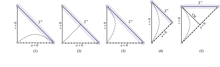
Figure 1: Conformal diagrams of a flat FLRW universe $a=(\bar{t}/\bar{t}_{0})^{p}$ for (1) $0<p<1/2$, (2) $p=1/2$, (3) $1/2<p<1$, (4) $p=1$ and (5) $p>1$. The dotted and dotted-dashed lines denote the trapping horizon, $r_{\rm TH}(\bar{t})=({\rm d}a/{\rm d}\bar{t})^{-1}$, and the big-bang singularity at $a=0$, respectively. The cases (2) and (4) correspond respectively to the radiation-dominant universe $P=\rho/(D-1)$ and the marginally accelerating universe driven by the curvature term $\rho\propto a^{-2}$. The cosmological horizon, $r_{\rm CH}(\bar{t})=(p-1)^{-1}\bar{t}_{0}(\bar{t}/\bar{t}_{0})^{1-p}$, is abbreviated to CH, which exists only in the strictly accelerating case ($p>1$). The shaded regions corresponding to $r\to\infty$ approximate our original spacetime.

On the other hand, taking the limit $r_{(i)}:=|\,\!\!\!\mbox{ \boldmath$x$}-\,\!\!\!\mbox{ \boldmath$x$}_{(i)}|\to 0$, we can safely neglect the time-dependence of the metric. Hence, the metric at the very neighborhood of each mass point is approximated by the Nariai-Bertotti-Robinson metric Nariai ; BR [the direct product of a 2-dimensional anti-de Sitter (AdS₂) and a ($D-2$)-sphere] as

$${\rm d}s^{2}_{r_{(i)}\to 0}=-\frac{r_{(i)}^{2}}{\ell_{(i)}^{2}}{\rm d}t^{2}+\frac{\ell_{(i)}^{2}}{r_{(i)}^{2}}{\rm d}r_{(i)}^{2}+\ell_{(i)}^{2}{\rm d}\Omega_{D-2}^{2}\,,$$ (31)

where $\ell_{(i)}:=[(Q_{T}^{(i)})^{n_{T}}(Q_{S}^{(i)})^{n_{S}}]^{1/[2(D-2)]}$ sets the curvature scale of ${\rm AdS}_{2}$ and ${\rm S}^{2}$ at the $i$-th point, and ${\rm d}\Omega_{D-2}^{2}$ is the line-element of a $(D-2)$-dimensional unit sphere. It has been noticed that the neighborhood of any extremal black holes can be universally described by the above metric Kunduri:2007vf ; Astefanesei:2007bf . Figure 2 compares the geometry of the AdS${}_{2}\times{\rm S}^{D-2}$ and that of the extremal RN black hole.

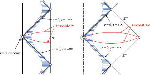
Figure 2: Typical “throat” geometries for the AdS${}_{2}\times{\rm S}^{D-2}$ spacetime (left) and the extremal RN spacetime (right). The double line stands for the degenerate horizon. Only the vicinity of the shaded point at $r=0$ with $t$ kept finite approximates our original solution. Whereas, the domains bounded by blue shaded lines in each figure are locally isometric Carter .

Thus, one anticipates that the metric (12) describes a system of charged black holes with a degenerate event horizon embedded in the FLRW universe filled by a fluid (30), which might lead us to speculate that the causal structure is found simply by patching Figures 1 and 2. As pointed out in MN , however, this naïve expectation fails if a single point mass is placed at $r=0$ for $D=4$ and $n_{T}=1$. The solution in MOU has neither a degenerate event horizon at $r=0$, nor a big-bang singularity at $t=0$. As is clear from Figure 2, the limit $r\to 0$ with $t$ kept finite does not describe the $(D-1)$-dimensional null surface (the blue shaded domain corresponding to $r\to 0$ with $|t|$ going to infinity), but describes only the point at the “throat infinity.” This lies at the core of why the present metric admits nonvanishing Hawking temperature. In order to elucidate the full causal structure, one has to discuss these null surfaces with much care, the analysis of which is the principal subject of this paper.

A curious property of the present solution (12) is that the field equations are completely linearized. One may encounter the linear gravitational equations in the context of the solitonic configurations and the supersymmetric solutions. In the present case, none of these interpretation fails. Despite the non-trivial time dependence, we are able to superpose the harmonics ad arbitrium. This property might be seemingly contradictory. Yet, one faces the same situation in the Kastor-Traschen solution KT , where the black hole collision can be described by multicenter harmonics. These spacetimes maintain a special balance in close analogy with supersymmetric states.

We will postpone the discussion regarding the multiple black holes in a separated paper. In this article, we shall limit our attention to the simplest case in which the harmonics $H_{A}$’s possess only a monopole term $\propto Q_{A}/r^{D-3}$ at the coordinate center, i.e., the spacetime is spherically symmetric. In this single-mass case for each harmonic, it is sufficient to consider the case of identical charges $Q_{T}=Q_{S}=:Q$, since $Q_{T}\neq Q_{S}$ amounts to a trivial conformal change

$$g_{\mu\nu}~{}\to~{}(Q_{T}/Q_{S})^{n_{T}/(D-2)}g_{\mu\nu}\,,$$ (32)

with the parameter redefinitions

$$t~{} \to(Q_{T}/Q_{S})^{-n_{T}/2}\,t\,,$$ (33)

$$t_{0} \to~{}(Q_{T}/Q_{S})^{1-n_{T}/2}\,t_{0}\,.$$ (34)

Thus, we will be concerned with the metric,

$${\rm d}s^{2}=-\Xi^{D-3}{\rm d}t^{2}+\Xi^{-1}\left({\rm d}r^{2}+r^{2}{\rm d}\Omega_{D-2}^{2}\right)\,,$$ (35)

where

$$\Xi=\left(H_{T}^{n_{T}}H_{S}^{n_{S}}\right)^{-1/(D-2)}\,,$$ (36)

with

$$H_{T}: =\frac{t}{t_{0}}+\frac{Q}{r^{D-3}}\,,$$ (37)

$$H_{S}: =1+\frac{Q}{r^{D-3}}\,.$$ (38)

The constant $Q$ has a physical meaning as a U$(1)$ charge, satisfying

$$\frac{Q}{\sqrt{G}}=\frac{1}{(D-3)\Omega_{D-2}}\int_{S}e^{\lambda_{A}\kappa\Phi}F_{\mu\nu}^{(A)}{\rm d}S^{\mu\nu}\,,$$ (39)

where $S$ is an arbitrary closed surface surrounding $r=0$, and

$$\Omega_{D-2}=\frac{2\pi^{(D-1)/2}}{\Gamma[(D-1)/2]}$$ (40)

denotes the area of a $(D-2)$-dimensional unit sphere. The above first integral is a direct consequence of Eq. (5). Though the charge may take either sign, we shall restrict ourselves to the positive case ($Q>0$) for definiteness of our argument.

III Matter fields and singularities

Let us first evaluate matter fields and discuss energy conditions. Next, we shall discuss the spacetime singularity.

III.1 Energy conditions

Many candidates of “black hole solutions” in the expanding universe found in the literature (Sultana-Dyer solution SultanaDyer , McVittie’s solution Mcvittie1933 , etc) do not respect energy conditions in the whole of spacetime. It is therefore worthwhile to argue whether the present spacetime satisfies suitable energy conditions.

Since the explicit metric-form is available, we can immediately evaluate the matter contents of the solution. Let us consider a (nongeodesic) observer whose integral curve is tangent to $\partial/\partial t$. The energy densities and the pressures for this observer are given by

$$\rho^{(\Phi)} =\frac{1}{2}\left[\Xi^{-(D-3)}(\Phi_{,t})^{2}+\Xi(\Phi_{,r})^{2}\right]+V$$

$$=\mbox{$\mathcal{F}$}_{1}+\mbox{$\mathcal{F}$}_{2}+\mbox{$\mathcal{F}$}_{3}>0\,,$$ (41)

$$P_{r}^{(\Phi)} =\frac{1}{2}\left[\Xi^{-(D-3)}(\Phi_{,t})^{2}+\Xi(\Phi_{,r})^{2}\right]-V$$

$$=\mbox{$\mathcal{F}$}_{1}+\mbox{$\mathcal{F}$}_{2}-\mbox{$\mathcal{F}$}_{3}\,,$$ (42)

$$P_{\Omega}^{(\Phi)} =\frac{1}{2}\left[\Xi^{-(D-3)}(\Phi_{,t})^{2}-\Xi(\Phi_{,r})^{2}\right]-V$$

$$=\mbox{$\mathcal{F}$}_{1}-\mbox{$\mathcal{F}$}_{2}-\mbox{$\mathcal{F}$}_{3}\,,$$ (43)

$$\rho^{(\rm em)} =-P_{r}^{(\rm em)}=P_{\Omega}^{(\rm em)}$$

$$=\mbox{$\mathcal{F}$}_{4}>0\,,$$ (44)

where the comma denotes the partial derivative, and

$$\mbox{$\mathcal{F}$}_{1}:= \frac{n_{T}n_{S}(D-3)}{8\kappa^{2}(D-2)t_{0}^{2}}\left(\frac{H_{S}}{H_{T}}\right)^{n_{S}(D-3)\over(D-2)}\,,$$ (45)

$$\mbox{$\mathcal{F}$}_{2}:= \frac{n_{T}n_{S}Q^{2}(D-3)^{3}(H_{T}-H_{S})^{2}}{8\kappa^{2}(D-2)r^{2(D-2)}H_{T}^{2+{n_{T}\over(D-2)}}H_{S}^{2+{n_{S}\over(D-2)}}}\,,$$ (46)

$$\mbox{$\mathcal{F}$}_{3}:= \frac{n_{T}(n_{T}-1)}{4\kappa^{2}t_{0}^{2}}\left(\frac{H_{S}}{H_{T}}\right)^{n_{S}(D-3)\over(D-2)}\,,$$ (47)

$$\mbox{$\mathcal{F}$}_{4}:= \frac{(D-3)^{2}Q^{2}\left(n_{T}H_{S}^{2}+n_{S}H_{T}^{2}\right)}{4\kappa^{2}r^{2(D-2)}H_{T}^{2+{n_{T}\over(D-2)}}H_{S}^{2+{n_{S}\over(D-2)}}}\,.$$ (48)

Here, the subscript $\Omega$ represents any of the angular components, which are all equal under the spherical symmetry. Due to the scalar field, the observer sees the nonvanishing energy flux, whose radial component $\mbox{$\mathcal{F}$}_{5}:=-\Xi^{-(D-4)/2}T_{tr}$ is found to be

$$\mbox{$\mathcal{F}$}_{5}=-\frac{n_{T}n_{S}Q(D-3)^{2}(H_{T}^{n_{T}}H_{S}^{n_{S}})^{(D-4)\over(D-2)}(H_{T}-H_{S})}{4\kappa^{2}(D-2)t_{0}r^{D-2}H_{T}^{2}H_{S}}\,.$$ (49)

From these, one can derive the following useful relations

$$\mbox{$\mathcal{F}$}_{1}+\mbox{$\mathcal{F}$}_{3}=\frac{n_{T}^{2}(D-1)}{8\kappa^{2}(D-2)t_{0}^{2}}\left(\frac{H_{S}}{H_{T}}\right)^{n_{S}(D-3)\over(D-2)}\,,$$ (50)

$$\mbox{$\mathcal{F}$}_{4}-\mbox{$\mathcal{F}$}_{2}=\frac{(D-3)^{2}Q^{2}H_{ST}^{2}}{8\kappa^{2}(D-2)r^{2(D-2)}H_{T}^{2+{n_{T}\over(D-2)}}H_{S}^{2+{n_{S}\over(D-2)}}}\,,$$ (51)

$$(\mbox{$\mathcal{F}$}_{1}-\mbox{$\mathcal{F}$}_{2})^{2}=(\mbox{$\mathcal{F}$}_{1}+\mbox{$\mathcal{F}$}_{2})^{2}-\mbox{$\mathcal{F}$}_{5}^{2}\,,$$ (52)

where we have used a shorthand notation

$$H_{ST}:=n_{S}H_{T}+n_{T}H_{S}\,.$$ (53)

Note that $\mbox{$\mathcal{F}$}_{1},\mbox{$\mathcal{F}$}_{2},\mbox{$\mathcal{F}$}_{4}$, $\mbox{$\mathcal{F}$}_{1}+\mbox{$\mathcal{F}$}_{3}$ and $\mbox{$\mathcal{F}$}_{4}-\mbox{$\mathcal{F}$}_{2}$ are positive-definite, while $\mbox{$\mathcal{F}$}_{3}$ is negative for $0<n_{T}<1$.

At the time $t=t_{0}$ we have $H_{T}=H_{S}$, hence the physical quantities evaluated at $t=t_{0}$ are reminiscent of those for the extremal RN solution. We shall refer to the time $t=t_{0}$ as a fiducial time. At $t=t_{0}$, the energy density of the scalar field is uniform in space as

$$\kappa^{2}\rho^{(\Phi)}={(D-1)n_{T}^{2}\over 8(D-2)t_{0}^{2}}\,,$$ (54)

and that of the electromagnetic field is the same as the extremal RN solution,

$$\kappa^{2}\rho^{(\rm em)}=\frac{(D-2)(D-3)Q^{2}}{2(r^{D-3}+Q)^{2(D-2)/(D-3)}}\,.$$ (55)

For $t>t_{0}$, $\mbox{$\mathcal{F}$}_{5}$ becomes negative, indicative of the scalar field falling into the black hole. As it turns out in the later section, this is not the case since the black-hole event horizon is a Killing horizon. Killing horizons represent “equilibrium states” of event horizons, precluding the black hole to grow wald2 . Physically considering, the accretion of the scalar field is delicately in balance on the horizon with the repulsive forces caused by the U$(1)$ fields.

We are now ready to discuss energy conditions for the total energy-momentum tensor. For the observer moving along $\partial/\partial t$, the total energy density and the pressures are given by

$$\rho =\rho^{(\Phi)}+\rho^{(\rm em)}\,,$$ (56)

$$P_{r} =P_{r}^{(\Phi)}+P_{r}^{(\rm em)}\,,$$ (57)

$$P_{\Omega} =P_{\Omega}^{(\Phi)}+P_{\Omega}^{(\rm em)}.$$ (58)

The simplest and the most intuitive one is the weak energy condition HE , which states that the energy density for an arbitrary observer with worldline $V^{\mu}$ is non-negative,

$$T_{\mu\nu}V^{\mu}V^{\nu}\geq 0\,.$$ (59)

Solving the characteristic equation $\det({T^{\mu}}_{\nu}-\mbox{$\mathcal{T}$}{\delta^{\mu}}_{\nu})=0$, we can diagonalize the (total) stress-energy tensor as ${T^{\hat{\mu}}}_{\hat{\nu}}={\rm diag}(-\hat{\rho},\hat{P}_{r},\hat{P}_{\Omega},...,\hat{P}_{\Omega})$, where the eigenvalues are given by

$$\hat{\rho} =\frac{1}{2}\left[\rho-P_{r}+\sqrt{(\rho+P_{r})^{2}-4\mbox{$\mathcal{F}$}_{5}^{2}}\right]\,,$$ (60)

$$\hat{P}_{r} =\frac{1}{2}\left[-(\rho-P_{r})+\sqrt{(\rho+P_{r})^{2}-4\mbox{$\mathcal{F}$}_{5}^{2}}\right]\,,$$ (61)

$$\hat{P}_{\Omega} =P_{\Omega}\,.$$ (62)

In terms of these quantities, the weak energy condition reads HE

$$\hat{\rho}\geq 0\,,\qquad\hat{\rho}+\hat{P}_{r}\geq 0\,,\qquad\hat{\rho}+\hat{P}_{\Omega}\geq 0\,.$$ (63)

From Eqs. (51) and (58) one obtains

$$[(\rho+P_{r})^{2}-4\mbox{$\mathcal{F}$}_{5}^{2}]^{1/2}=2|\mbox{$\mathcal{F}$}_{1}-\mbox{$\mathcal{F}$}_{2}|\,.$$ (64)

Noticing $\mbox{$\mathcal{F}$}_{4}-\mbox{$\mathcal{F}$}_{2}>0$, it follows that the last two inequalities in Eq. (63) hold. Then, it remains to examine the positivity of $\hat{\rho}=\mbox{$\mathcal{F}$}_{3}+\mbox{$\mathcal{F}$}_{4}+|\mbox{$\mathcal{F}$}_{1}-\mbox{$\mathcal{F}$}_{2}|$, or a lack thereof. In the region $\mbox{$\mathcal{F}$}_{1}-\mbox{$\mathcal{F}$}_{2}\geq 0$, we have

$$\hat{\rho}=(\mbox{$\mathcal{F}$}_{1}+\mbox{$\mathcal{F}$}_{3})+(\mbox{$\mathcal{F}$}_{4}-\mbox{$\mathcal{F}$}_{2})>0\,,$$ (65)

while in the region $\mbox{$\mathcal{F}$}_{1}-\mbox{$\mathcal{F}$}_{2}<0$, we have

$$\hat{\rho}=-\mbox{$\mathcal{F}$}_{1}+\mbox{$\mathcal{F}$}_{2}+\mbox{$\mathcal{F}$}_{3}+\mbox{$\mathcal{F}$}_{4}\,.$$ (66)

At first sight, the sign of $\mbox{$\mathcal{F}$}_{3}+\mbox{$\mathcal{F}$}_{4}$ might be obscure in the latter case. Yet, using the condition $\mbox{$\mathcal{F}$}_{1}-\mbox{$\mathcal{F}$}_{2}<0$, it turns out to be bounded below as

$$\mbox{$\mathcal{F}$}_{3}+\mbox{$\mathcal{F}$}_{4} >\left[\frac{n_{T}H_{S}^{2}+n_{S}H_{T}^{2}+n_{T}(n_{T}-1)(H_{T}-H_{S})^{2}}{4\kappa^{2}t_{0}^{2}}\right]\left(\frac{H_{S}}{H_{T}}\right)^{n_{S}(D-3)\over(D-2)}\,,$$ (67)

$$=\left[\frac{(n_{S}-n_{T})H_{T}^{2}+2n_{T}H_{T}H_{S}+n_{T}^{2}(H_{T}-H_{S})^{2}}{4\kappa^{2}t_{0}^{2}}\right]\left(\frac{H_{S}}{H_{T}}\right)^{n_{S}(D-3)\over(D-2)}\,.$$ (68)

From Eq. (67) the positivity of $\hat{\rho}$ immediately follows for $n_{T}\geq 1$. In the case of $n_{T}<1$ [$n_{S}>(D-1)/(D-3)$], observing the inequality

$$n_{S}-n_{T}>\frac{D-1}{D-3}-1=\frac{2}{D-3}>0\,,$$ (69)

we are led to the conclusion $\hat{\rho}>0$ from Eq. (68). Hence, the weak energy condition is satisfied in either case.

One can evaluate other types of energy conditions in a similar fashion. In the background FLRW universe, the acceleration of the universe is driven when timelike convergence condition ceases to be valid HE . In general relativity this condition is equivalent to saying that the strong energy condition

$$\left(T_{\mu\nu}-\frac{1}{D-2}{T^{\rho}}_{\rho}g_{\mu\nu}\right)V^{\mu}V^{\nu}\geq 0\,,$$ (70)

is violated, indicative of peculiar matter fields with large negative pressures. In terms of eigenvalues of the stress-energy tensor, the strong energy condition amounts to

$$\hat{\rho}+\hat{P}_{r}\geq 0\,,\qquad\hat{\rho}+\hat{P}_{\Omega}\geq 0\,,$$

$$(D-3)\hat{\rho}+\hat{P}_{r}+(D-2)\hat{P}_{\Omega}\geq 0\,.$$ (71)

The last condition is rewritten as

$$(D-3)\hat{\rho}+\hat{P}_{r}+(D-2)\hat{P}_{\Omega}$$

$$~{}=(D-2)\left(|\mbox{$\mathcal{F}$}_{1}-\mbox{$\mathcal{F}$}_{2}|+\mbox{$\mathcal{F}$}_{1}-\mbox{$\mathcal{F}$}_{2}\right)$$

$$~{}~{}~{}~{}+2\left[-\mbox{$\mathcal{F}$}_{3}+(D-3)\mbox{$\mathcal{F}$}_{4}\right]\,.$$ (72)

In the case of $\mbox{$\mathcal{F}$}_{1}-\mbox{$\mathcal{F}$}_{2}>0$, a straightforward calculation reduces the right-hand side of the above equation to

$$8t_{0}^{2}\kappa^{2}H_{T}^{2+{n_{T}\over(D-2)}}H_{S}^{2+{n_{S}\over(D-2)}}\left[(D-2)(\mbox{$\mathcal{F}$}_{1}-\mbox{$\mathcal{F}$}_{2})-\mbox{$\mathcal{F}$}_{3}+(D-3)\mbox{$\mathcal{F}$}_{4}\right]$$

$$~{}~{}=\frac{(D-3)^{3}Q^{2}t_{0}^{2}}{r^{2(D-2)}}\left\{2(n_{T}H_{S}^{2}+n_{S}H_{T}^{2})-n_{T}n_{S}(H_{T}-H_{S})^{2}\right\}-(D-1)n_{T}(n_{T}-2)H_{T}^{n_{T}}H_{S}^{n_{S}+2}\,.$$ (73)

Since the last term on the right-hand side of Eq. (73) is always dominant for $r\to\infty$, the strong energy condition violates if $n_{T}>2$, i.e., when the background FLRW universe is accelerating $(p>1)$. While, for $n_{T}\leq 2$, i.e., when the background FLRW universe is decelerating $(p\leq 1)$, we can conclude that the strong energy condition holds, following the same line of argument as Eqs. (65)–(69) (note that we must also evaluate the case of $\mbox{$\mathcal{F}$}_{1}-\mbox{$\mathcal{F}$}_{2}<0$). Namely, the present spacetime satisfies the strong energy condition if and only if the background FLRW universe does.

As shown above, it is dependent on the parameters and restricted to the particular spacetime regions whether the strong (and the dominant) energy condition holds. The failure of these energy conditions is, however, not so serious. It is widely accepted that the minimal requirement to avoid any pathologies is the null energy condition: $\hat{\rho}+\hat{P}_{r}\geq 0$ and $\hat{\rho}+\hat{P}_{\Omega}\geq 0$. If the null energy condition is not satisfied, undesirable instabilities would develop NEC . Since the present system satisfies the weak energy condition, the null energy condition automatically holds HE . Hence, the present spacetime is free from such annoying plagues. This motivates us to study the system as a physically acceptable one.

III.2 Misner-Sharp energy

A celebrated quantity that characterizes the matter fields in spherical symmetry is the Misner-Sharp quasilocal energy MS1964 . The advantage of the use of Misner-Sharp energy is that it also characterizes the local spacetime structure Hayward1994 ; hideki ; nozawa . The quasilocal energy is interpreted as a gravitational energy contained within a closed surface. Especially when the spacetime fails to admit globally conserved charges, the quasilocal energy is a helpful local measure to identify matter distributions.

A major superiority in spherical symmetry lies in the fact that we can define covariantly the circumference radius as

$$R:=r\Xi^{-1/2}$$ (74)

Using the above circumference radius, the $D$-dimensional Misner-Sharp quasilocal energy, $m$, is given by hideki

$$m=\frac{D-2}{2\kappa^{2}}\Omega_{D-2}R^{D-3}\left[1-g^{\mu\nu}(\nabla_{\mu}R)(\nabla_{\nu}R)\right]\,.$$ (75)

The Misner-Sharp mass is defined uniquely by the metric components and its first derivatives, and does not require the asymptotic conditions of spacetime. Once the spherical surface specified by the circumference radius is fixed, the Misner-Sharp mass is given without ambiguity. Such a quasi-localization is possible on account of spherical symmetry, in which no gravitational wave is generated.

The present spacetime metric (12) yields

$$m= \frac{\Omega_{D-2}|r|^{D-3}}{8(D-2)t_{0}^{2}\kappa^{2}r^{2(D-1)}H_{T}^{2-[(D-3)n_{T}]/[2(D-2)]}H_{S}^{2-[(D-3)n_{S}]/[2(D-2)]}}$$

$$\times\left[n_{T}^{2}r^{2D}H_{T}^{n_{T}}H_{S}^{n_{S}+2}+4(D-2)(D-3)Qr^{D+1}t_{0}^{2}H_{T}H_{S}H_{ST}-(D-3)^{2}Q^{2}r^{4}t_{0}^{2}H_{ST}^{2}\right]\,.$$ (76)

We can provide each term in Eq. (76) with physical interpretation by evaluating at the fiducial time $t=t_{0}$, at which the Misner-Sharp energy reduces to

$$m(t_{0},R)= \frac{\Omega_{D-2}n_{T}^{2}r^{D-1}H_{S}^{(D-1)/(D-3)}}{8(D-2)\kappa^{2}t_{0}^{2}}+\frac{D-2}{2\kappa^{2}H_{S}}\Omega_{D-2}Q+\frac{D-2}{2\kappa^{2}}\Omega_{D-2}Q$$

$$= \frac{\Omega_{D-2}}{D-1}R^{D-1}\rho^{(\Phi)}(t_{0})+\Omega_{D-2}\int^{R}_{Q^{1/(D-3)}}{\rm d}RR^{D-2}\rho^{(\rm em)}(t_{0},R)+\frac{(D-2)\Omega_{D-2}}{2\kappa^{2}}Q\,.$$ (77)

The first term in the above equation corresponds to the energy of the scalar field, and the last two terms to the U$(1)$ energies outside and inside the black hole.

For $Q=0$, only the first term in Eq. (76) survives, yielding

$$m =\frac{(D-2)\Omega_{D-2}a^{D-3}r^{D-1}}{2\kappa^{2}}\left(\frac{{\rm d}a}{{\rm d}\bar{t}}\right)^{2}$$

$$=\frac{\Omega_{D-2}}{D-1}(ar)^{D-1}\rho^{(\Phi)}\,,$$ (78)

as expected for the background FLRW universe. This implies also that the first term in Eq. (76) is the contribution of a scalar field.

III.3 Curvature singularities

We can see easily that the dilaton profile (19) and the square of the electromagnetic fields

$$F^{(T)}_{~{}\mu\nu}F^{(T)\mu\nu} =-\frac{4\pi(D-3)^{2}Q^{2}}{r^{2(D-2)}}\left(\frac{H_{S}^{n_{S}(D-4)}}{H_{T}^{(4-n_{T})D+4(n_{T}-2)}}\right)^{1/(D-2)}\,,$$ (79)

$$F^{(S)}_{~{}\mu\nu}F^{(S)\mu\nu} =-\frac{4\pi(D-3)^{2}Q^{2}}{r^{2(D-2)}}\left(\frac{H_{T}^{n_{T}(D-4)}}{H_{S}^{(4-n_{S})D+4(n_{S}-2)}}\right)^{1/(D-2)}\,,$$ (80)

diverge at

$$t=t_{s}(r):=-Q/r^{D-3},~{}~{}{\rm and}~{}~{}~{}r^{D-3}=-Q\,.$$ (81)

One may thence deduce that these surfaces correspond to the genuine spacetime singularities characterized by the divergence of scalar quantities of curvature. As a simple illustration, let us see the square of the Weyl-tensor

$$\mbox{$\mathcal{C}$}_{\mu\nu\rho\sigma}\mbox{$\mathcal{C}$}^{\mu\nu\rho\sigma}={(D-3)\over(D-1)}\,\mbox{$\mathcal{W}$}^{2}\,,$$ (82)

where (see e.g., appendix of hideki for derivation)

$$\mbox{$\mathcal{W}$}=-\frac{(D-3)Q\left[(D-3)Qr^{3}\left\{H_{ST}^{2}+2(n_{S}H_{T}^{2}+n_{T}H_{S}^{2})\right\}-2(D-1)r^{D}H_{T}H_{S}H_{ST}\right]}{2r^{2D-1}H_{T}^{2+n_{T}/(D-2)}H_{S}^{2+n_{S}/(D-2)}}\,.$$ (83)

One finds that the the above curvature invariant quantity necessarily blows up at (81), where the inverse of the lapse function vanishes. Since the circumference radius vanishes at (81), these two singularities are both sitting at the physical center $R=0$. The other curvature scalar quantities (e.g. $\mbox{$\mathcal{R}$}_{abcd}\mbox{$\mathcal{R}$}^{abcd}$ and $\mathcal{R}$) do indeed diverge at these central points.

It is notable to remark that the $t=0$ surface is completely regular, since the curvature invariants are bounded therein. The nonzero U$(1)$ charge smoothenes the big-bang singularity which exists in the background expanding universe (see Figure 1). Note also that the null surface $r=0$ is not singular, as in the case of MN . We may therefore extend the spacetime across the $r^{D-3}=0$ surface, i.e., the negative $r$ region for even dimensions, and the $r^{2}<0$ region for odd dimensions.

Accordingly, the allowed coordinate regions are $H_{T}^{n_{T}}H_{S}^{n_{S}}>0$, which is arranged to give

$$t>t_{s}(r)~{}~{}{\rm with}~{}~{}~{}r^{D-3}>-Q$$ (84)

or

$$t<t_{s}(r)~{}~{}{\rm with}~{}~{}~{}r^{D-3}<-Q\,.$$ (85)

We are not interested in the latter domain since it turns out to be disconnected with the outside region $r>0$ by the singularity. For this reason, we shall focus on the coordinate ranges

$$t>t_{s}(r)\,,\qquad r^{D-3}>-Q\,,$$ (86)

Next, it is important to address the causal structure of these singularities. We can intuitively expect that both of these singularities have the timelike structure, since the Misner-Sharp mass is unbounded below as approaching these singularities. To establish the timelike signature of singularities, it is sufficient to show that there exist an infinite number of radial null geodesics stemming from and terminating into the singularities MN ; NM .

In the vicinity of the singularity $r=-Q^{1/(D-3)}$, let us assume the following asymptotic form of the radial null geodesics,

$$r+Q^{1/(D-3)}=C_{0}(t-t_{1})^{q}\,,$$ (87)

where $q(>0)$ and $C_{0}$ are constants. Substituting this ansatz into the outgoing radial null condition ${\rm d}r/{\rm d}t=\Xi^{(D-2)/2}$, we obtain

$$q =\frac{2}{n_{S}+2}\,,$$

$$C_{0}^{1+n_{S}/2} =\frac{n_{S}+2}{2}Q^{n_{S}/2}\left(1-\frac{t_{1}}{t_{0}}\right)^{-n_{T}/2}\,.$$ (88)

This verifies that infinite geodesics parametrized by the departure time $t_{1}(<t_{0})$ emanate from the singularity. For the ingoing null geodesics, we can also arrive at the conclusion that there exist infinite ingoing null geodesics running into the singularity. The proof proceeds similarly for the singularity $t=t_{s}(r)$: it is shown that there exist infinite ingoing and outgoing geodesics falling into and emerging from the singularity at the time $t>t_{0}$ for $r<0$ and at the time $t<0$ for $r>0$. It follows that both of these two singularities have a timelike structure, i.e., these are locally naked singularities. As argued in HH , these timelike singularities are associated with the U$(1)$ charge, not with the background universe.

In order to verify whether these singularities are visible to observer far in the distance from the central region, we have to trace the geodesics all the way out to infinity. We will numerically confirm in later section that the singularities $t_{s}(r)$ and $r=-Q^{1/(D-3)}$ lying in the $r<0$ region are contained inside the black hole. On the other hand, we will see that the singularity $t_{s}(r)$ emerging in the $r>0$ region is not covered by the event horizon.

IV Spacetime structures

We shall explore the spacetime structure of the “black hole candidate” (12). In order to conclude that the present spacetime is indeed qualified as a black hole, we need to appreciate the infinite future of the spacetime to assess the locus of the event horizon. Thus, the notion of event horizon is of less practical use especially in the time-evolving spacetimes. In the dynamical spacetime where the null geodesic motions are not solved analytically, it is much more advantageous to focus on the trapped surface, which is locally defined and hence free from such a difficulty. When a catastrophic gravitational collapse occurs to form a black hole, there arises a region where even “outgoing” null rays are dragged back due to strong gravity of the black hole. These null rays with negative expansion will be absorbed into the hole, characterizing the intuitive idea of the black hole as a region of no escape. For each time slice, this surface defines an apparent horizon HE as an outermost boundary of the trapped region in the asymptotically flat spacetimes. Hayward generalized these quasilocal notions to define a class of trapping horizons Hayward1993 . Trapping horizons are associated not only with black holes but also with white holes and cosmological ones, suitable for the present context.

Since the event horizons and trapping horizons are conceptually different, there is no a priori relationship between them (the black hole in stationary spacetime is exceptional, for which the event horizon and the trapping horizon coincide HE ; HIW ). Nevertheless, we can rely on the Hawking’s theorem that all trapped surfaces appear inside a black hole under the null energy condition provided the spacetime is asymptotically flat with some additional technical assumptions (see Proposition 9.2.8 in HE for the proof). Although the present spacetime is not asymptotically flat, taking into the fact that the metric is well-behaved off of the central singularity at $R=0$, this criterion is of use for our study. This expectation will be backed by numerical analysis of null geodesic motions.

For simplicity of our argument, we shall focus our attention only to the 4-dimensional case. We also assume $t_{0}>0$ and $Q>0$. We define dimensionless variables $\tilde{t}:=t/t_{0}$, $\tilde{r}:=r/Q$ and work in the dimensionless metric $Q^{-2}{\rm d}s^{2}=:{\rm d}\tilde{s}^{2}=\tilde{g}_{\mu\nu}{\rm d}\tilde{x}^{\mu}{\rm d}\tilde{x}^{\nu}$ to simplify our discussion. To be specific, we work in the metric

$${\rm d}\tilde{s}^{2}=-\tau^{2}\Xi{\rm d}\tilde{t}^{2}+\Xi^{-1}\left[{\rm d}\tilde{r}^{2}+\tilde{r}^{2}\left({\rm d}\theta^{2}+\sin^{2}\theta{\rm d}\phi^{2}\right)\right]\,,$$ (89)

where

$$\tau:=\frac{t_{0}}{Q}\,,\qquad\Xi=\frac{\tilde{r}^{2}}{[(\tilde{t}\tilde{r}+1)^{n_{T}}(\tilde{r}+1)^{n_{S}}]^{1/2}}\,,$$ (90)

with

$$n_{T}+n_{S}=4\,,$$ (91)

for which the dimensionless circumference radius is defined by

$$\tilde{R}=[(\tilde{t}\tilde{r}+1)^{n_{T}}(\tilde{r}+1)^{n_{S}}]^{1/4}\,.$$ (92)

The metric is parametrized by two dimensionless parameters $\tau$ and $n_{T}$. In what follows, dimensionless variables associated with the metric (89) will be denoted with tilde.

The physical meaning of $\tau$ is naïvely given as follows. The energy density of the scalar field at $t=t_{0}$ is $\rho^{(\Phi)}\propto 1/t_{0}^{2}$ [Eq. (54)]. While, for the extreme RN black hole with the charge $Q$, the total energy density of the U(1) fields evaluated on the horizon is given by $\kappa^{2}\rho^{\rm(em)}|_{\scriptscriptstyle H}\propto 1/Q^{2}$ [Eq. (55)]. Thus for the time-dependent black hole we can claim that $\tau$ is related to the ratio of two energy densities at the event horizon as

$$\tau^{2}\sim{\rho^{\rm(em)}\over\rho^{(\Phi)}}\Big{|}_{\scriptscriptstyle H}\,.$$ (93)

A more rigorous treatment shown below [see Eq. (132)] confirms that the above estimate is indeed true.

Before going to the detailed analysis, we classify our spacetimes into nine types [from Case I-(i) to Case III-(iii)]. Classification of Cases I–III is dependent on the expansion rate of the universe, i.e., whether the universe is decelerating ($n_{T}<2$), marginal ($n_{T}=2$) or accelerating ($n_{T}>2$). The parameter $\tau$ is also important in the subclassification for each Class I–III, whereby the global structures of the solution change drastically. We summarize our classification in Table 1, which includes some important results given later.

IV.1 Trapping horizons

A trapped surface is defined on a closed and orientable spacelike surface $S$. Since the present spacetime admits an SO$(3)$-symmetry, we take $S$ as a metric sphere. Let us introduce the Newman-Penrose null tetrads as

$$l_{\mu}{\rm d}\tilde{x}^{\mu} =\sqrt{\frac{\Xi}{2}}(-\tau{\rm d}\tilde{t}+\Xi^{-1}{\rm d}\tilde{r})\,,$$

$$n_{\mu}{\rm d}\tilde{x}^{\mu} =\sqrt{\frac{\Xi}{2}}(-\tau{\rm d}\tilde{t}-\Xi^{-1}{\rm d}\tilde{r})\,,$$ (94)

$$m_{\mu}{\rm d}\tilde{x}^{\mu} =\frac{\tilde{r}}{\sqrt{2\Xi}}({\rm d}\theta+i\sin\theta{\rm d}\phi)\,,$$

with $\bar{m}_{\mu}$ being a complex conjugate of $m_{\mu}$. These null vectors satisfy $l^{\mu}n_{\mu}=-1=-m^{\mu}\bar{m}_{\mu}$. $l^{\mu}$ and $n^{\mu}$ are the future-directed radial null vectors. Using these tetrads, expansions are defined by

$$\tilde{\theta}_{+}:=2m^{(\mu}\bar{m}^{\nu)}\tilde{\nabla}_{\mu}l_{\nu}\,,\qquad\tilde{\theta}_{-}:=2m^{(\mu}\bar{m}^{\nu)}\tilde{\nabla}_{\mu}n_{\nu}\,,$$ (95)

where the operation of “Re” has been omitted because the vanishing rotation is obvious. The present metric (89) computes to give

$$\tilde{\theta}_{\pm}=\frac{n_{T}\tilde{r}^{2}H_{S}\sqrt{H_{T}^{n_{T}}H_{S}^{n_{S}}}\pm\tau\left(4\tilde{r}H_{T}H_{S}-H_{ST}\right)}{2\sqrt{2}\tau\tilde{r}^{2}H_{T}^{1+n_{T}/4}H_{S}^{1+n_{S}/4}}\,.$$ (96)

These expansions characterize the rate of divergence of outgoing and ingoing light rays. It should be remarked, however, that values of expansions themselves are not invariant quantities due to the relative normalization of $l^{\mu}$ and $n^{\mu}$. Only their product

$$\tilde{\theta}_{+}\tilde{\theta}_{-}=-2\tilde{R}^{-2}(\tilde{\nabla}_{\mu}\tilde{R})(\tilde{\nabla}^{\mu}\tilde{R})$$ (97)

has a covariant meaning.

A metric sphere is said to be trapped (untrapped) if $\tilde{\theta}_{+}\tilde{\theta}_{-}>0$ ($\tilde{\theta}_{+}\tilde{\theta}_{-}<0$), and marginal when $\tilde{\theta}_{+}\tilde{\theta}_{-}=0$. A trapping horizon is the closure of a hypersurface foliated by marginal surfaces, i.e., trapping horizons occur at $\tilde{\theta}_{\pm}=0$.

It is instructive first to see the case of FLRW universe ($Q=0$), in which only $\theta_{-}=0$ has a solution

$$r_{\rm TH}={4t_{0}\over n_{T}}\,\left(\frac{t}{t_{0}}\right)^{\,1-{n_{T}/2}}\,.$$ (98)

Using the relations (25) and (28), the trapping horizon is expressed in terms of the cosmic time $\bar{t}$ as $r_{\rm TH}=p^{-1}\bar{t}_{0}(\bar{t}/\bar{t}_{0})^{1-p}$. Written in the the circumference radius $R=ar$, this is translated into

$$R_{\rm TH}=a\left(\frac{{\rm d}a}{{\rm d}\bar{t}}\right)^{-1}\,,$$ (99)

which is the Hubble horizon as desired. This kind of trapping horizon is associated to the background universe–the past trapping horizon in the terminology of Hayward Hayward1994 –manifesting a situation that even the ingoing null rays are pushed outwards due to the cosmic expansion.

Unfortunately, for $Q\neq 0$ it is not feasible to obtain the orbits of trapping horizons in the explicit analytic form $\tilde{t}=\tilde{t}_{\rm TH}(\tilde{r})$ unless $n_{T}$ takes an integer. Reminding that the trapping horizons occur where $\tilde{\nabla}_{\mu}\tilde{R}$ becomes null, we find that it is more helpful to express the positions of trapping horizons in terms of the circumference radius $\tilde{R}$. Now, $\tilde{t}$ is expressed by $\tilde{R}$ and $\tilde{r}$ as

$$\tilde{t}=\frac{1}{\tilde{r}}\left\{\left[\frac{\tilde{R}^{4}}{(\tilde{r}+1)^{n_{S}}}\right]^{1/n_{T}}-1\right\}\,.$$ (100)

Inserting this relation into Eq. (12), we can write the metric in terms of $\tilde{r}$ and $\tilde{R}$ as

$${\rm d}\tilde{s}^{2}= -\tau^{2}\biggl{[}\frac{{\rm d}\tilde{r}}{\tilde{r}\tilde{R}}\left\{1-\frac{\tilde{R}^{4/n_{T}}(n_{T}+4\tilde{r})}{n_{T}(\tilde{r}+1)^{4/n_{T}}}\right\}$$

$$+\frac{4\tilde{R}^{n_{S}/n_{T}}{\rm d}\tilde{R}}{n_{T}\tilde{R}(\tilde{r}+1)^{n_{S}/n_{T}}}\biggr{]}^{2}+\frac{\tilde{R}^{2}}{\tilde{r}^{2}}{\rm d}\tilde{r}^{2}+\tilde{R}^{2}{\rm d}\Omega_{2}^{2}\,.$$ (101)

Setting $\tilde{R}={\rm constant}$, one obtains the induced metric of the constant $\tilde{R}$ surfaces,

Table 1: Classification of the spacetime structures of the solution (89). The parameter $n_{T}$ corresponds to the steepness parameter of the dilaton potential, which is related to the expansion exponent of the FLRW universe $a\propto\bar{t}^{p}$ as Eq. (28), while $\tau:=t_{0}/Q$ measures the “nonextremality” of the black hole. This classification is based on the spacetime structures discussed in the text. In the last column, “BH” and “NS” represent whether the spacetime describes a regular black hole or a naked singularity without an event horizon.

Case		$n_{T}$	$\tau$	number of	causal structure
				horizons	infinity	near-horizon	global structure
extreme RN		$n_{T}=0$	any	1	Minkowski	Fig. 2 (left)	Fig. 2 (right)	: BH
I	(i)	$0<n_{T}<4/3$			Fig. 1(1)
(decelerating universe: $p<1$)	(ii)	$n_{T}=4/3$	any	2	Fig. 1(2)	Fig. 5(A)	Fig. 7(a)	: BH
	(iii)	$4/3<n_{T}<2$			Fig. 1(3)
II	(i)		$\tau>1$	2		Fig. 5(A)	Fig. 7(a)	: BH
(Milne universe: $p=1$)	(ii)	$n_{T}=2$	$\tau=1$	1	Fig. 1(4)	Fig. 5(B)	Fig. 7(b)	: NS
	(iii)		$\tau<1$			Fig. 5(C)
III	(i)		$\tau>\tau_{\rm cr}$	3		Fig. 5(D)	Fig. 7(d)	: BH
(accelerating universe: $p>1$)	(ii)	$2<n_{T}<4$	$\tau=\tau_{\rm cr}$	2	Fig. 1(5)	Fig. 5(E)	Fig. 7(e)	: BH
	(iii)		$\tau<\tau_{\rm cr}$	1		Fig. 5(C)	Fig. 7(c)	: NS
RNdS		$n_{T}=4$	any	3	dS	n/a	Fig. 5(D)	: BH

$${\rm d}\tilde{s}^{2}_{R}=-\frac{1}{\tilde{R}^{2}\tilde{r}^{2}}\left[\tau^{2}\left\{\frac{\tilde{R}^{4/n_{T}}(n_{T}+4\tilde{r})}{n_{T}(1+\tilde{r})^{4/n_{T}}}-1\right\}^{2}-\tilde{R}^{4}\right]{\rm d}\tilde{r}^{2}\,,$$ (102)

where we have discarded the angular parts which are irrelevant to the discussion of trapping horizon.

Figure 3 depicts the $\tilde{R}-\tilde{r}$ diagram, from which we can read off the signature of $\tilde{R}={\rm constant}$ surfaces. From Eq. (97), the region where the $\tilde{R}={\rm constant}$ surface is timelike (spacelike) consists of the untrapped (trapped) surfaces. The thick lines in Figure 3 designate the loci of trapping horizons at which the terms in square-bracket of Eq. (102) vanish, ${\rm d}\tilde{s}^{2}_{R}=0$. The spacetime has at most three types of trapping horizons, $\tilde{R}_{2}(\tilde{r})\leq\tilde{R}_{1,-}(\tilde{r})\leq\tilde{R}_{1,+}(\tilde{r})$, where $\tilde{R}_{2}(\tilde{r})$ satisfies

$$\tau\left[\frac{\tilde{R}_{2}(\tilde{r})^{4/n_{T}}(n_{T}+4\tilde{r})}{n_{T}(1+\tilde{r})^{4/n_{T}}}-1\right]+\tilde{R}_{2}(\tilde{r})^{2}=0\,,$$ (103)

whereas $\tilde{R}_{1,-}(\tilde{r})$ and $\tilde{R}_{1,+}(\tilde{r})$ are two positive roots (if they exist) of the equation

$$\tau\left[\frac{\tilde{R}_{1}(\tilde{r})^{4/n_{T}}(n_{T}+4\tilde{r})}{n_{T}(1+\tilde{r})^{4/n_{T}}}-1\right]-\tilde{R}_{1}(\tilde{r})^{2}=0\,.$$ (104)

Observe that the definition of $\tilde{R}_{1}(\tilde{r})$ and $\tilde{R}_{2}(\tilde{r})$ differs from that in the previous paper MN , where $\tilde{R}_{1}(\tilde{r})$ and $\tilde{R}_{2}(\tilde{r})$ were defined by the surfaces of $\tilde{\theta}_{-}=0$ and $\tilde{\theta}_{+}=0$, respectively. In the $\tilde{r}<0$ region, the surfaces $\tilde{R}_{1}(\tilde{r})$ and $\tilde{R}_{2}(\tilde{r})$ defined by Eqs. (104) and (103) are not always coincident with the $\tilde{\theta}_{-}=0$ and $\tilde{\theta}_{+}=0$ surfaces. Still, it is found that in the $\tilde{r}>0$ region $\tilde{\theta}_{-}=0$ holds at $\tilde{R}_{1}(\tilde{r})$ and $\tilde{\theta}_{+}=0$ holds at $\tilde{R}_{2}(\tilde{r})$.

Figure 3: Typical plots of circumference radius $\tilde{R}$ (vertical axis) against $\tilde{r}$ (horizontal axis) for Case I-(i) ($n_{T}=1$ with $\tau=1$), Case II-(i) ($n_{T}=2$ with $\tau=3/2$), Case II-(ii) ($n_{T}=2$ with $\tau=1$), Case II-(iii) ($n_{T}=2$ with $\tau=1/2$), Case III-(i) ($n_{T}=3$ with $\tau=3$), Case III-(ii) ($n_{T}=3$ with $\tau=\tau_{\rm cr}$) and Case III-(iii) ($n_{T}=3$ with $\tau=1$). The curve of Case I-(i) is the representative for Case I. The thick lines denote trapping horizons, across which the $\tilde{R}={\rm constant}$ surface changes the signature. The region “spacelike” (and respectively “timelike”) stands for the domain where the $\tilde{R}={\rm constant}$ surfaces are spacelike (timelike). In Case III-(i), the bounded region tends to shrink as $\tau$ decreases and eventually degenerate into a point shown in Case III-(ii).

In Figure 3 we display seven plots of trapping horizons according to the classification shown in Table 1. [We have dropped Cases I-(ii) and I-(iii) because these plots are the same as that for Case I-(i).] Our previous paper MN discussed the spacetime with $n_{T}=1$ belonging to Case I-(i), where two trapping horizons $\tilde{R}_{1,-}(\tilde{r})$ and $\tilde{R}_{2}(\tilde{r})$ arise. Case II-(i) behaves similarly as Case I. The universe in Case II undergoes a marginal acceleration $a\propto\bar{t}$. Our main interest is toward Case III, where the background FLRW universe is accelerating. Figure 3 illustrates that the region $\tilde{R}>\tilde{R}_{1,+}(\tilde{r})$ with $\tilde{r}>0$ is composed of trapped surfaces, in accordance with the acceleration of the background FLRW universe.

Let us uncover the properties of these trapping horizons. Looking at Eq. (103), one finds that the trapping horizon $\tilde{R}_{2}(\tilde{r})$ approaches to the constant $\tilde{R}_{2}(\tilde{r})\to\sqrt{\tau}$ in the limit of $\tilde{r}\to\infty$. Noting the inequality ${\rm d}\tilde{R}_{2}(\tilde{r})/{\rm d}\tilde{r}>0$ for $\tilde{r}>0$, $\tilde{R}_{2}(\tilde{r})\leq\sqrt{\tau}$ is concluded in the $\tilde{r}>0$ region. In Case I ($n_{T}<2$), ${\rm d}\tilde{R}/{\rm d}\tilde{r}<(>)0$ holds for $\tilde{R}_{2}<(>)\tilde{R}_{2,<}$ in the region $\tilde{r}<0$, where

$$\tilde{R}_{2,<}:=\sqrt{\frac{2\tau}{2-n_{T}}}\,.$$ (105)

While, for $n_{T}\geq 2$, ${\rm d}\tilde{R}_{2}/{\rm d}\tilde{r}<0$ holds in the $\tilde{r}<0$ region. Thus, in every case the trapping horizon $\tilde{R}_{2}(\tilde{r})$ develops and diverges as $\tilde{r}\to-n_{T}/4$.

It is easy to find that $\tilde{R}_{1,+}(\tilde{r})$ is confluent with $\tilde{R}_{1,-}(\tilde{r})$ at the constant radius $\tilde{R}=\tilde{R}_{1,>}$, where

$$\tilde{R}_{1,>}:=\sqrt{\frac{2\tau}{n_{T}-2}}\,.$$ (106)

at which $\tilde{R}_{1,\pm}(\tilde{r})$ has a vertical tangent. Hence, the largest trapping horizon $\tilde{R}_{1,+}(\tilde{r})$ exists if and only if $n_{T}>2$. For $n_{T}<2$ and $n_{T}=2$ with $\tau>1$, the trapping horizon $\tilde{R}_{1,-}(\tilde{r})$ diverges as $r\to-n_{T}/4$. For $n_{T}>2$, ${\rm d}\tilde{R}_{1,-}/{\rm d}\tilde{r}>(<)0$ and ${\rm d}\tilde{R}_{1,+}/{\rm d}\tilde{r}<(>)0$ hold in the region $\tilde{r}>(<)0$. Denoting $\tilde{R}_{-}:=\tilde{R}_{2}(0)$, $\tilde{R}_{+}:=\tilde{R}_{1,-}(0)$ and $\tilde{R}_{c}:=\tilde{R}_{1,+}(0)$, it then follows that $\tilde{R}_{+}<\tilde{R}_{1,-}(\tilde{r})<\tilde{R}_{1,+}(\tilde{r})<\tilde{R}_{c}$ for Case III-(i).

The signature of trapping horizons is an important issue to be discussed. Differentiating Eq. (103), we obtain the expression of ${\rm d}\tilde{R}_{2}/{\rm d}\tilde{r}$ along the trapping horizon. Substituting this into the metric (101), we can find the induced metric on the trapping horizon. After a simple but tedious algebra, we obtain

$${\rm d}\tilde{s}^{2}_{\rm TH}=-\frac{4(1+\tilde{r})^{2}}{n_{S}\tilde{r}^{2}\tilde{R}_{2}^{4}}\biggl{[} n_{T}\tilde{R}_{2}^{4}+2\tilde{R}_{2}^{2}(\tau-\tilde{R}_{2}^{2})$$

$$+\frac{4n_{S}\tilde{r}^{2}(\tau-\tilde{R}_{2}^{2})^{2}}{(n_{T}+4\tilde{r})^{2}}\biggr{]}{\rm d}\tilde{R}_{2}^{2}\,.$$ (107)

It immediately follows that the cases of $n_{T}\geq 2$ and $n_{T}<2$ with $\tilde{R}<\tilde{R}_{2,<}$ assure that the trapping horizon $\tilde{R}_{2}(\tilde{r})$ is always timelike ${\rm d}\tilde{s}_{\rm TH}^{2}<0$. We can numerically check that $\tilde{R}_{2,-}$ is timelike also for $\tilde{R}>\tilde{R}_{2,<}$.

Similarly, along the trapping horizon $\tilde{R}_{1}$, we have

$${\rm d}\tilde{s}^{2}_{\rm TH}=-\frac{4(1+\tilde{r})^{2}}{n_{S}\tilde{r}^{2}\tilde{R}_{1}^{4}}\biggl{[} n_{T}\tilde{R}_{1}^{4}-2\tilde{R}_{1}^{2}(\tau+\tilde{R}_{1}^{2})$$

$$+\frac{4n_{S}\tilde{r}^{2}(\tau+\tilde{R}_{1}^{2})^{2}}{(n_{T}+4\tilde{r})^{2}}\biggr{]}{\rm d}\tilde{R}_{1}^{2}\,.$$ (108)

Inspecting Eq. (106), the trapping horizon $\tilde{R}_{1,+}$ is necessarily timelike. On the other hand, to see the signature of $\tilde{R}_{1,-}$, numerical calculation is necessary. Nevertheless, we can see the universal behavior around $\tilde{r}=0$, where the last term in the square bracket of Eq. (108) is negligible. Taking into account Eq. (106), it is found that $\tilde{R}_{1,-}$ is spacelike near $\tilde{r}=0$.

An analytic estimation is possible for the background FLRW universe $Q=0$, for which Eq. (108) reduces to

$${\rm d}s^{2}_{\rm TH}=\frac{4-3n_{T}}{n_{S}}{\rm d}R_{1}^{2}\,,$$ (109)

implying that the signature of trapping horizon is timelike for $p>1/2$ ($n_{T}>4/3$), spacelike for $p<1/2$ ($n_{T}<4/3$) and null for $p=1/2$ ($n_{T}=4/3$). This accounts for the subclassification of Case I shown in Fig. 1. The behaviors of trapping horizon $\tilde{R}_{1,-}$ in the asymptotic region are analogous to those in the FLRW case.

IV.2 Event horizons

In order to identify the locus of event horizon, we follow the strategy laid out in our previous paper MN . We shall first discuss the geometry of the near-horizon metric and demonstrate that the null surfaces of “event-horizon candidate” in our dynamical spacetime (89) are described by the Killing horizons. Our next tactics is to confirm these local horizons are indeed qualified as true horizons in the original spacetime by computing the null geodesic motions numerically. These logical steps will guide us in the right direction for obtaining the global causal structure.

IV.2.1 Near-horizon geometry

The analysis in Sec. II reveals that the limit $\tilde{r}\to 0$ and $\tilde{t}$ being finite corresponds to the “throat” geometry. This fact leads us to speculate that the event horizons in the present spacetime, if exist, correspond to the null surfaces at $\tilde{r}\to 0$ with $\tilde{t}\to\pm\infty$, i.e., the infinite redshift and blueshift surfaces “joined” at the throat. To discuss these null surfaces in more detail, it is useful to take the near-horizon limit, defined by

$$\tilde{t}~{}\to~{}\frac{\tilde{t}}{\epsilon}\,,\qquad\tilde{r}~{}\to~{}\epsilon\tilde{r}\,,\qquad\epsilon~{}\to~{}0\,.$$ (110)

After the rescalings, the metric is free from $\epsilon$, and we can obtain the near-horizon geometry

$${\rm d}\tilde{s}_{\rm NH}^{2}= -\tau^{2}\tilde{r}^{2}(1+\tilde{t}\tilde{r})^{-n_{T}/2}{\rm d}\tilde{t}^{2}$$

$$+\tilde{r}^{-2}(1+\tilde{t}\tilde{r})^{n_{T}/2}\left({\rm d}\tilde{r}^{2}+\tilde{r}^{2}{\rm d}\Omega_{2}^{2}\right)\,.$$ (111)

As a direct corollary of the scaling limit (110), the near-horizon metric (111) admits a Killing vector

$$\xi^{a}=\tilde{t}\left(\frac{\partial}{\partial\tilde{t}}\right)^{a}-\tilde{r}\left(\frac{\partial}{\partial\tilde{r}}\right)^{a}\,.$$ (112)

By a straightforward calculation, we find that the above Killing field is hypersurface-orthogonal

$$\xi_{[\mu}\mbox{$\mathcal{D}$}_{\nu}\xi_{\rho]}=0\,,$$ (113)

where $\mbox{$\mathcal{D}$}_{\mu}$ is a derivative operator of the near-horizon metric (111). Hence, by transforming to the new coordinates

$$\tilde{T}=\pm\ln|\tilde{t}|+\int^{\tilde{R}}\frac{4\tilde{R}^{3+4/n_{T}}{\rm d}\tilde{R}}{n_{T}(\tilde{R}^{4/n_{T}}-1)f(\tilde{R})}\,,$$

$$\tilde{R}=(1+\tilde{t}\tilde{r})^{n_{T}/4}\,,$$ (114)

where

$$f(\tilde{R}):=\tau^{2}\left(\tilde{R}^{4/n_{T}}-1\right)^{2}-\tilde{R}^{4}\,,$$ (115)

we can bring the near-horizon metric (111) into a manifestly static form,

$${\rm d}\tilde{s}^{2}=-\frac{f(\tilde{R})}{\tilde{R}^{2}}{\rm d}\tilde{T}^{2}+\frac{16\tau^{2}\tilde{R}^{8/n_{T}}}{n_{T}^{2}f(\tilde{R})}{\rm d}\tilde{R}^{2}+\tilde{R}^{2}{\rm d}\Omega_{2}^{2}\,.$$ (116)

In this coordinate system, the Killing vector (112) is expressed as $\xi^{\mu}=(\partial/\partial\tilde{T})^{\mu}$. It is obvious that the above metric (116) describes a static spacetime with Killing horizons at $f(\tilde{R})=0$ where the Killing vector $\xi^{\mu}$ becomes null. It deserves to note that terms in square bracket in Eq. (102) simplify to $f(\tilde{R})$ in the near horizon limit. This means that the trapping horizons tend to be null as approaching $\tilde{r}\to 0$, in accordance with the results in the previous subsection.

Since $\tilde{t}$ and $\tilde{r}$ are not gauge-invariant quantities, one may be worried about whether the scaling limit (110) is indeed well-defined. This prescription of “zooming-up” can be justified as follows. In the scaling limit (110), the dilaton and the U$(1)$ fields reduce to

$$\kappa\Phi=\sqrt{\frac{2n_{S}}{n_{T}}}\ln\tilde{R}\,,$$ (117)

and

$$\kappa\tilde{F}_{\tilde{T}\tilde{R}}^{(T)}=\frac{4\sqrt{2\pi}\tau}{n_{T}\tilde{R}^{1+4/n_{T}}}\,,\quad~{}~{}\kappa\tilde{F}^{(S)}_{\tilde{T}\tilde{R}}=\frac{4\sqrt{2\pi}\tau}{n_{T}R^{1-4/n_{T}}}\,.$$ (118)

We can confirm that the spacetime (116) with (117) and (118) still satisfies the field equations of Einstein-“Maxwell”-dilaton gravity (3)–(5). This warrants that the near-horizon limit (110) is not the singular procedure since it maps the original metric (12) onto another one (111) in the same theory. Note that the case $n_{T}=4$ does not yield the near-horizon metric, since the metric (111) is identical to the original one (89) and simply giving rise to a static chart of the RNdS black hole with $M=Q$.

Let us devote some space to discuss the near-horizon geometry in more detail. Although the near-horizon metric (111) is neither asymptotically flat nor asymptotically AdS, the global causal structures reduce to those of known solutions. Such unusual asymptotic structures of black holes are commonly found when the dilaton field is present Chan:1995fr ; Yazadjiev:2005du ; soda . The near-horizon metric (111) admits horizons at $f(\tilde{R})=0$, which is rewritten into the equation

$$F_{\pm}(\tilde{R})=\tau\,,~{}~{}{\rm with}~{}~{}~{}F_{\pm}(\tilde{R}):=\frac{\pm\tilde{R}^{2}}{\tilde{R}^{4/n_{T}}-1}\,.$$ (119)

This equation gives the candidates for horizon radius, $\tilde{R}_{-}$, $\tilde{R}_{+}$, and $\tilde{R}_{c}$, which were found in the limit of $r\rightarrow 0$ of the trapping horizons in the previous subsection. The number of roots for Eq. (119) [or $f(\tilde{R})=0$] can be seen visually as the intersection points of $F_{\pm}(\tilde{R})$ and $\tau={\rm constant}$ (see Figure 4).

Irrespective of the values of $\tau$ and $n_{T}$, behavior of $F_{-}$ is universal: it starts from zero and diverges as $\tilde{R}\to 1$. Then, $F_{-}(\tilde{R})=\tau$ has always a solution $\tilde{R}=\tilde{R}_{-}$ less than unity. Whereas, the behavior of $F_{+}$ depends on the value of $n_{T}$, i.e., $n_{T}<2$, $n_{T}=2$ or $n_{T}>2$. As is clear from Figure 4, for $n_{T}<2$ [Case I in Table 1] and $n_{T}=2$ with $\tau>1$ [Case II-(i)], we find two horizons ($\tilde{R}_{-}$ and $\tilde{R}_{+}$). When $n_{T}=2$ and $\tau\leq 1$ [Cases II-(ii) and (iii)], we have only one root ($\tilde{R}_{-}$). In the case of $n_{T}>2$, where the background universe is accelerating, $F_{+}$ has a minimum at

$$\tilde{R}=\tilde{R}_{\rm cr}:=\left(\frac{n_{T}}{n_{T}-2}\right)^{n_{T}/4}\,.$$ (120)

Hence, for

$$\tau>\tau_{\rm cr}:=\frac{1}{2}n_{T}^{n_{T}/2}(n_{T}-2)^{1-n_{T}/2}\,.$$ (121)

the equation (119) has three distinct roots, $\tilde{R}_{-}<\tilde{R}_{+}\leq\tilde{R}_{c}$ [Case III-(i)]. When $\tau=\tau_{\rm cr}$, two horizons $\tilde{R}_{+}$ and $\tilde{R}_{c}$ become degenerate [Case III-(ii)]. If $\tau<\tau_{\rm cr}$, we have only one root [Case II-(iii)]. These results are shown in Table 1.

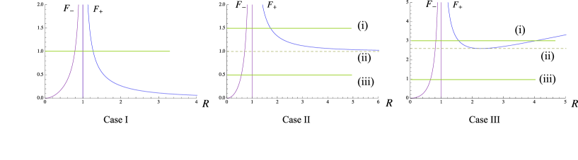
Figure 4: Plots of $F_{+}$ and $F_{-}$ for Case I (left), Case II (middle) and Case III (right) (see Table 1 for classification). The equality $f(\tilde{R})=0$ then possesses two distinct solutions for Case I and Case II-(i), a single solution for Cases II-(ii), II-(iii) and III-(iii), three distinct solutions for Case III-(i) and two solutions with larger one being degenerate for Case III-(ii).

The spacetime structure of the near-horizon metric for each case I–III is obtained by simple evaluation of radial null geodesics (see e.g., TM ). We will not devote much time to discussing this issue since our primary interest in this subsection is exclusively to the horizon structure. We obtain 5 types of conformal diagrams, as shown in Figure 5 (A)–(E). The figure (A) corresponds to Cases I and II-(i), (B) to Case II-(ii), (C) to Case II-(iii) and III-(iii), (D) to Case III-(i) and (E) to Case III-(ii). These classifications are also included in Table 1. Despite the nontrivial asymptotic structures (116), these conformal diagrams are identical to the familiar solutions. The figure (A) is the same as the RN-AdS, (B) as the vanishing mass RN spacetime with a hyperbolic horizon, (C) as the negative mass SdS, (D) as the nonextremal RNdS and (E) as the degenerate RNdS, respectively. The surfaces $\tilde{R}_{+}$ and $\tilde{R}_{-}$ are the black hole event horizon and the white hole horizon for the near-horizon geometry and also for the original metric. It should be emphasized, however, that the largest horizon $\tilde{R}_{c}$ does not approximate our original metric, since the surface $\tilde{R}_{c}$ corresponds to the limit $\tilde{t}\to 0$ and $\tilde{r}\to\infty$ with $\tilde{t}\tilde{r}$ being finite in the near-horizon geometry (the green line in Figure 5). It incidentally arises due to the symmetry of the near-horizon metric not shared by the original metric. Consequently, the null surface $\tilde{R}_{c}$ is irrelevant to the cosmological horizon in the original metric (89), although it is a cosmological horizon for the near-horizon metric. It is worth commenting also that the case $n_{T}=n_{S}=2$ with $\tau=1$ is special, for which there exists “internal null infinity” $\mbox{$\mathcal{I}$}^{+}_{\rm in}$ specified by $\tilde{t}\to\infty$ and $\tilde{r}\to 0$ with $\tilde{R}=(\tilde{t}\tilde{r}+1)^{1/2}$ being infinite. This surface has an outgoing null structure. Only the ingoing null geodesics can approach $\mbox{$\mathcal{I}$}^{+}_{\rm in}$, hence it should be distinguished by $\mbox{$\mathcal{I}$}^{+}_{\rm out}$ ($\tilde{t}\to\infty$ and $\tilde{r}\to\infty$). The Carter-Penrose diagram in this case is given in Figure 5(B).

To conclude, the neighborhoods of the null surfaces $\tilde{R}_{+}$ and $\tilde{R}_{-}$ in the original metric (89) are locally isometric to the corresponding null surfaces–these are indeed the Killing horizons–in the near-horizon metric (111) or (116). In Figure 5, only the shaded regions in the vicinity of the horizon approximate our original metric (89). The surface $\tilde{R}_{+}$, if exists, deserves a black-hole event horizon for the near-horizon metric and it turns out later, this surface corresponds to a black hole horizon for the original metric as well.

Note also that the vector field $\xi^{\mu}$ (112) solves the Killing equation in the original spacetime only at the horizon. Since the outside region is highly dynamical, it comes as a surprise for us that the unexpected Killing symmetry arises. This is achieved due to the fact that the electromagnetic repulsive force and the cosmic expansion are compensated by the gravitational and dilatonic attraction. These Killing horizons $\tilde{R}_{\pm}$ are in general nondegenerate in the sense that the surface gravities $\tilde{\kappa}_{\pm}$ are nonvanishing. From the formula

$$2\tilde{\kappa}^{2}_{\pm}=\mp(\tilde{\nabla}_{\mu}\xi_{\nu})(\tilde{\nabla}^{\mu}\xi^{\nu})\,,$$ (122)

one obtains the surface gravities associated with $\xi^{\mu}$ as

$$\tilde{\kappa}_{\pm}=1\mp\frac{n_{T}\tilde{R}^{2-4/n_{T}}_{\pm}}{2\tau}\,.$$ (123)

These are nonvanishing unless $\tau=\tau_{\rm cr}$. The surface gravities are constant over the horizon, as expected.

IV.2.2 Null geodesics

The argument given in previous subsection strongly implies that $\tilde{R}_{+}$ and $\tilde{R}_{-}$ are the future and past event horizons. In order to conclude this in a more rigorous manner, we need to discuss geodesic motions. Since the present spacetime admits a spherical symmetry, it is sufficient to focus on the radial null geodesics to determine the causal structure.

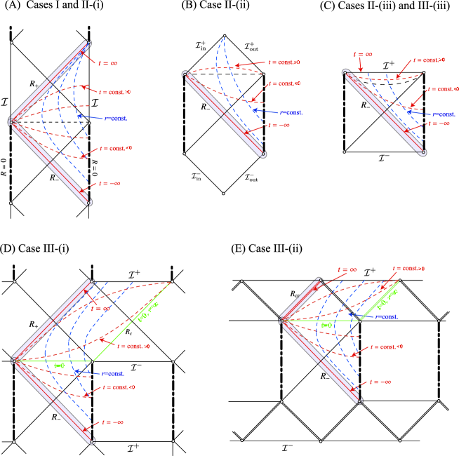
Figure 5: Conformal diagrams of the maximally extended near-horizon geometries. The global structures are the same as those for (A) the nonextremal RN-AdS, (B) the zero-mass RN spacetime with a “hyperbolic horizon,” (C) the negative mass SdS (or the overcharged RNdS), (D) the nonextremal RNdS and (E) the extremal RNdS. The thick dotted-dashed lines denote the central singularity at $\tilde{t}=-1/r$. The shaded regions approximate our original solution (89).

Using the relation for the radial null vectors,

$$\tau\dot{\tilde{t}}=\pm\sqrt{H_{T}^{n_{T}}H_{S}^{n_{S}}}\dot{\tilde{r}}\,,$$ (124)

the radial null geodesic equations simplify to

$$\ddot{\tilde{t}}\pm\frac{\tau H_{ST}}{2\tilde{r}^{2}(H_{T}^{n_{T}+2}H_{S}^{n_{S}+2})^{1/2}}\dot{\tilde{t}}^{2} = 0\,,$$ (125)

$$\ddot{\tilde{r}}\pm\frac{n_{T}(H_{T}^{n_{T}}H_{S}^{n_{S}})^{1/2}}{2\tau H_{T}}\dot{\tilde{r}}^{2} = 0\,,$$ (126)

Here and hereafter, the plus (minus) sign refers to as the outgoing (ingoing) null geodesics, and the dot means the differentiation with respect to an affine parameter $\lambda$.

Following MN ; Brill the asymptotic geodesic behavior around the surface $\tilde{R}_{+}$ (corresponding to $\tilde{t}\to\infty$ and $\tilde{r}\to 0$) can be evaluated as

$$\tilde{r}=c_{1}^{(+)}(\lambda-\lambda_{+})^{1/\tilde{\kappa}_{+}}\,,\qquad\tilde{t}=c_{2}^{(+)}(\lambda-\lambda_{+})^{-1/\tilde{\kappa}_{+}}\,,$$ (127)

where $c_{1,2}^{(+)}$ is constant, $\lambda_{+}$ corresponds to the arrival time at $\tilde{R}_{+}$ and $\tilde{\kappa}_{+}$ was defined by Eq. (123). This equation not only means that the horizon can be reached within a finite affine time but also that $\tilde{r}$ and $1/\tilde{t}$ are not the smooth functions of $\lambda$ at $\lambda_{+}$ (unless $\tilde{\kappa}_{+}^{-1}$ happens to be integral).

Let us move on to the numerical analysis. Exploiting the affine transformation, if necessary, we can impose without loss of any generality $\lambda=0$ at the starting point of the geodesics and $\dot{\tilde{t}}(0)=\pm 1$. Then the geodesics are distinguished by their initial point $[\tilde{t}(0),\tilde{r}(0)]$.

Our primary concern here is Case III, where the background universe is accelerating. We will give a detailed description exclusively of $n_{T}=3$ with $\tau=3$ [Case III-(i)]. We first develop geodesics for the outside region $\tilde{r}>0$ by setting the initial radial coordinate to be $\tilde{r}(0)=1$. It then follows that the $\tilde{r}=1$ surface is divided by three trapping horizons into four regions (see Figure 3). Take the representative spacetime points $p_{I}~{}(I=1,...4)$ specified by $(\tilde{t}_{I}(0),\tilde{r}(0)=1)$ with $t_{1}(0)>t_{2}(0)>t_{3}(0)>t_{4}(0)$ in such a way that $p_{I}$ is contained in each partitioned (un)trapped region. We shall refer to the geodesics starting from the initial point $p_{I}$ as “Class-$I$.” For $\tilde{r}<0$, we take $\tilde{r}(0)=-1/10$ and repeat the identical procedure with redefining “Class-$I$” as $t_{4}(0)<t_{3}(0)<t_{2}(0)<t_{1}(0)$. Figure 6 presents our numerical result in the accelerating universe ($n_{T}=\tau=3$) and the deduced Carter-Penrose diagrams are shown in Figure 7(d).

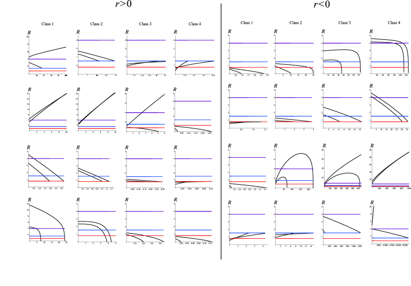
Figure 6: Behaviors of radial null geodesics for the accelerating universe ($n_{T}=3$ with $\tau=3$) in the outside region (left) and the inside region (right). The figures show the circumference radius versus the affine parameter. The red, blue and purple lines stand for $\tilde{R}_{-}\sim 0.82$, $\tilde{R}_{+}\sim 1.56$ and $\tilde{R}_{c}\sim 4.03$, respectively. The diagrams in the top, upper middle, lower middle, bottom rows correspond to future-directed ingoing null geodesics, future-directed outgoing null geodesics, past-directed ingoing null geodesics and past-directed outgoing null geodesics. We have shown the null geodesics for the initial values $\tilde{r}(0)=1$ (left) and $\tilde{r}(0)=-1/10$ (right).

Let us begin by the analysis for $\tilde{r}>0$. Among the Class-1 geodesics of the future-directed ingoing null, geodesics with a sufficiently large $\tilde{t}_{1}$ tend to diverge as the affine time evolves, while geodesics with $\tilde{t}_{1}(0)$ being close to the trapping horizon converge to $\tilde{R}_{+}$ with an infinite redshift. This implies the existence of a cosmological horizon [the $45^{\circ}$ line denoted by CH in Figure 7(d)], which is a characteristic feature in the accelerating universe as seen for the $p>1$ case in Figure 1. Other classes of geodesics unavoidably approach $\tilde{R}_{+}$ within a finite affine parameter.

Behaviors of future-directed outgoing null geodesics of Class-3 imply the existence a critical null curve [the black dotted $45^{\circ}$ line in Figure 7(d)] above which the geodesics can reach infinity and below which the geodesics inevitably plunge into the singularity $\tilde{t}=\tilde{t}_{s}(\tilde{r})$.

Motions of the past-directed ingoing null geodesics are universal: they necessarily get to the null surface $\tilde{R}_{-}$ with undergoing an infinite blueshift.

The past-directed outgoing null geodesics also exhibit a universal behavior: they inevitably reach the timelike singularity $\tilde{t}_{s}(\tilde{r})$ [the gray dashed-dotted line $\tilde{R}=0$ in Figure 7(d)] within a finite affine parameter.

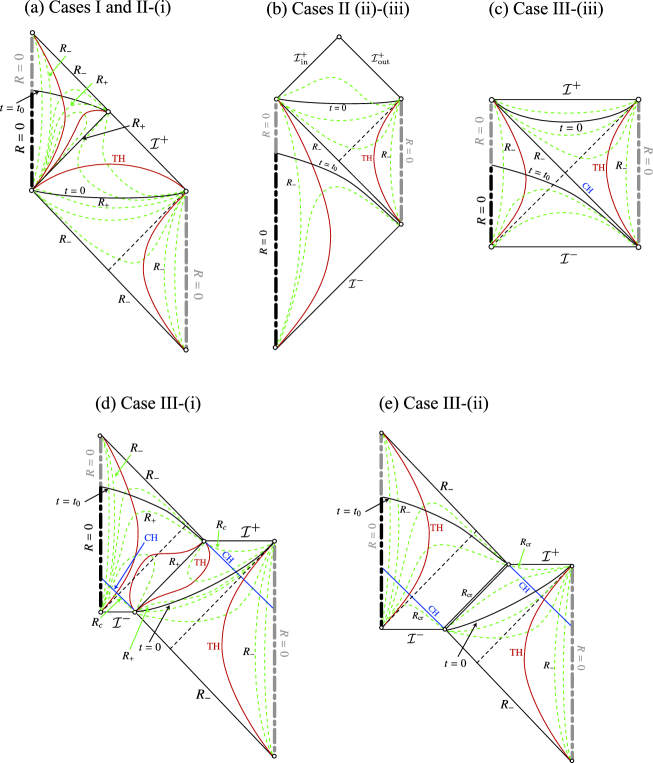
Figure 7: Conformal diagrams of the present spacetime (12) for Cases I–III. The green dotted curves stand for the $R={\rm constant}$ surfaces. The red thick curves represent the trapping horizons (TH) and blue lines denote the cosmological horizons (CH). The gray and black dotted-dashed curves correspond to the singularities of $r=-Q$ and $t=t_{s}(r)$, respectively. Figure (a), where the universe is decelerating, has been argued in the previous paper MN . For Figure (b), the universe undergoes a marginal acceleration $a\propto\bar{t}$. It admits an internal null infinity $\mbox{$\mathcal{I}$}^{+}_{\rm in}$ at which $r=0$ and $t\to\infty$ with $R\to\infty$. Figures (c)–(e) correspond to the accelerating universe. Figure (d) shows that there appear three horizons: the black hole horizon $R_{+}$, the “white hole horizon” $R_{-}$ and the cosmological horizon denoted by CH (not $R_{c}$). In Figure (e), the horizon is degenerate, while in Figure (c) the spacetime is overcharged to give a globally naked singularity. Figures (a), (d) and (e) are extensible across the surface $R_{-}$ with a contracting universe in a continuous but nonanalytic manner.

Assembling these results, we are able to draw a conformal diagram of Figure 7(d). The future infinity consists of a spacelike surface, consistent with the behavior of future-directed ingoing null geodesics of Class-1, and with the FLRW limit $\tilde{r}\to\infty$ as described in Figure 1(V). The timelike singularity $\tilde{t}_{s}(\tilde{r})=-1/\tilde{r}$ exists up to $\tilde{t}=0$, which is joined with $\mbox{$\mathcal{I}$}^{+}$. The cosmological horizon develops, whose orbit $\tilde{t}=\tilde{t}_{\rm CH}(\tilde{r})$ can be traced numerically. The green-dotted lines denote the $\tilde{R}={\rm constant}$ surfaces, which change signature across the trapping horizons. The $\tilde{R}={\rm constant}$ surfaces can be written in comparison with Figure 3, and the trapping horizons can be drawn from Eq. (107) and (108). The Carter-Penrose diagram explicitly shows that the null surface $\tilde{R}_{+}$ deserves to be a black hole horizon. The null surface $\tilde{R}_{-}$, on the other hand, may not suitable to be called a white hole horizon in a rigorous sense since the spacetime admits no past infinity in the outside region. Nevertheless, we shall stick to call it a “white hole horizon,” from the spirit of a one way membrane as a “region of no-entrance.”

The global structure of the solution in the inside region ($\tilde{r}<0$) can be deduced analogously. It is notable that the inside region admits a past null infinity $\mbox{$\mathcal{I}$}^{-}$. At first glance, it seems peculiar because the background universe is expanding (at $\mbox{$\mathcal{I}$}^{-}$ the circumference radius $\tilde{R}$ is already infinite there and the universe is not able to expand further!). We recognize that the spacetime indeed approaches to the expanding FLRW universe only in the limit of $r\to+\infty$ with $t/t_{0}>0$ [see Eq. (25)], while this is not true in the limit $t/t_{0}\to-\infty$ with $-1<\tilde{r}<0$, in which case the background geometry looks like a contracting universe.

Following the above treatment, one can draw the Carter-Penrose diagrams for other cases. We do not display those behaviors of null geodesics corresponding to Figure 6 in order to retain the compactness of the present paper, but they are easy to obtain. (Without geodesic analysis one can intuitively deduce the causal structures simply by inspecting the $\tilde{R}-\tilde{r}$ diagram in Figure 3). We have arrived at 5-types of global conformal diagrams shown in Figure 7 (a)–(e). Let us summarize the results.

Figure 7(a) corresponding to Cases I and II-(i) was given in our previous paper MN . The spacetime has a regular, nondegenerate event horizon $\tilde{R}_{+}$, and approaches to the decelerating FLRW universe. In the picture shown in Fig 7(a), we sketch the trapping horizons for the $n_{T}=\tau=1$ case, where the spacelike trapping horizon $\tilde{R}_{1}$ develops in the outside domain. Its signature depends sensitively on $n_{T}$ and $\tau$. For example, it becomes asymptotically null in the radiation-dominated case ($n_{T}=4/3$). Though the signature of trapping horizons is modified depending on the parameters, the causal structure remains unaltered.

In Figure 7(e) [Case III-(ii)], the spacetime has a degenerate event horizon at $\tilde{R}_{+}=\tilde{R}_{c}$ and asymptotically tends to the accelerating FLRW universe. This is a special situation of Case III-(i).

On the other hand, the spacetime fails to have a black hole horizon in Figures 7(b) [Cases II-(ii) and II-(iii)] and 7(c) [Case III-(iii)] (see Table 1). These cases correspond to spacetimes with naked singularities. In Figure 7(b) where $n_{T}=n_{S}=2$, one may recognize that there exists the “internal” null infinity $\mbox{$\mathcal{I}$}^{+}_{\rm in}$, where $\tilde{r}\to 0$ and $\tilde{t}\to\infty$ with $\tilde{R}\sim(\tilde{t}\tilde{r})^{1/2}\to\infty$. We can show the existence of $\mbox{$\mathcal{I}$}^{+}_{\rm in}$ as follows. Setting $n_{T}=n_{S}$ and assuming $\tilde{r}\sim 0$ with $\tilde{t}\to\infty$, one can find the asymptotic solutions of the radial ingoing null geodesics (125) and (126) around $\lambda\to\infty$ as

$$r=\lambda^{-\tau/(1-\tau)}\,,~{}~{}~{} {\rm with}~{}~{}~{}t=C_{1}\lambda^{1/(1-\tau)}\,,$$ (128)

for $\tau<1$, and

$$r=\frac{W(C_{2}\lambda)}{\lambda}\,,~{}~{}~{} {\rm with}~{}~{}~{}t=\lambda\,,$$ (129)

for $\tau=1$, where $C_{1}$ and $C_{2}$ are positive constants and $W$ is Lambert’s $W$-function satisfying $W(x)e^{W(x)}=x$. These asymptotic geodesics both satisfy $\tilde{t}\tilde{r}\to\infty$ as $\lambda\to\infty$. Whereas, the outgoing radial null geodesics do not decrease $\tilde{r}$. This proves the existence of $\mbox{$\mathcal{I}$}^{+}_{\rm in}$, at which only the ingoing null geodesics can arrive.

We have revealed that our solution (89) specified by three continuous parameters ($Q,n_{T},\tau$) describes a charged black hole in the FLRW universe in some parameter range. It is therefore worthwhile to discuss the physical meaning of these parameters. It is clear that the constant $Q$ is a U$(1)$ charge, whilst $n_{T}$ is the steepness of the dilaton potential (if $n_{T}$ happens to be natural number, it counts the number of time-dependent branes).

If $n_{T}=4$, the parameter $t_{0}$ has a clear meaning as a curvature radius of the de Sitter spacetime. However, the meaning of $\tau$ (or $t_{0}$) is less obvious for $n_{T}\neq 4$. In order to clarify the meaning, we shall consider the energy densities of two fields. The values of $\rho^{(\Phi)}$ and $\rho^{\rm(em)}$ on the event horizon $\tilde{R}_{+}$ are given by

$$\kappa^{2}\rho^{(\Phi)}|_{H} = {n_{T}(n_{T}+2)\over 8t_{0}^{2}}\tilde{R}_{+}^{-{2n_{S}/n_{T}}}\,,$$ (130)

$$\kappa^{2}\rho^{\rm(em)}|_{H} = {n_{S}+n_{T}\tilde{R}_{+}^{-{8/n_{T}}}\over 4Q^{2}\tilde{R}_{+}^{2}}\,,$$ (131)

which leads to

$${\rho^{\rm(em)}\over\rho^{(\Phi)}}\Big{|}_{H}={2\tau^{2}\over n_{T}(n_{T}+2)}\tilde{R}_{+}^{-4}\left(n_{T}+n_{S}\tilde{R}_{+}^{{8/n_{T}}}\right)\,.$$ (132)

The horizon radius $\tilde{R}_{+}$ is given in terms of $\tau$ via Eq. (119). As a result, we find that the ratio of two energy densities at the horizon is related to $\tau$, although the relation is complicated. In the limit of $\tau\rightarrow\infty$, however, we find a simple relationship

$${\rho^{\rm(em)}\over\rho^{(\Phi)}}\Big{|}_{H}\rightarrow{8\over n_{T}(n_{T}+2)}\,\tau^{2}\,.$$ (133)

Figure 8 depicts the dependence of ${\rho^{\rm(em)}/\rho^{(\Phi)}}$ against $\tau$. It follows that $\tau^{2}$ has a one to one correspondence to the ratio of two energy densities evaluated at the horizon $\tilde{R}_{+}$.

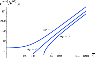
Figure 8: Relation between $\tau$ and the ratio of two energy densities at the horizon in the double logarithmic plot. This illustrates the almost linear relationship between $\tau^{2}$ and $\rho^{\rm(em)}/\rho^{(\Phi)}|_{H}$.

We can also give an afterthought implication to $\tau$ as follows. From Eq. (119), one obtains a relationship

$$\tau=\frac{\tilde{R}_{+}^{2}+\tilde{R}_{-}^{2}}{\tilde{R}_{+}^{4/n_{T}}-\tilde{R}_{-}^{4/n_{T}}}\,.$$ (134)

This equation implies that the parameter $\tau$ measures the “nonextremality” of the Killing horizon. An extremal limit is taken $\tau\to\infty$ where $\tilde{R}_{+}=\tilde{R}_{-}$ and $\tau\to\tau_{\rm cr}$ where $\tilde{R}_{+}=\tilde{R}_{c}$. Inferring from the supersymmetric case, the nonextremality indicates that the mass is strictly larger than the (central) charge. Hence, we deduce that some combination of the above parameters will give a well-defined mass of a black hole larger than the charge $Q$. Considering that the black hole horizon does not occur for small $\tau$, this point of view is supported. If a well-behaved mass definition is found, we are able to discuss the thermodynamics of a black hole. This expected possibility is now under investigation.

V Concluding Remarks

We have presented a family of solutions in a $D$-dimensional Einstein-“Maxwell”-dilaton system with a Liouville potential. In the single mass case, the solution interlies the extremal black hole and the FLRW universe with a power-law expansion. This solution reduces in the special cases to the extremal RN black hole ($n_{T}=0$), the nonextremal RNdS black hole ($n_{S}=0$) and the solution of MOU derived from the intersecting M-branes ($D=4$ and $n_{T}=1$). The present spacetime is characterized by three parameters: the steepness of the dilaton potential $n_{T}$, the U$(1)$ charge $Q$ and the “nonextremality” (or the ratio of two energy densities at the horizon) $\tau$. The parameter $n_{T}$ controls the expanding power $p$ of the background FLRW universe. For any choice of parameters, the system is shown to obey the weak energy condition.

The primary aim of this paper is to obtain global structures of the solution. The spacetime can be grouped into the nine cases [Cases I-(i)–III-(iii)] summarized in Table 1, according to the parameter values. Our consequence is visually captured in Figure 7, where the 5-types of global structure are obtained. In the case where the background universe is accelerating ($n_{T}>2$) with large nonextremality parameter ($\tau\geq\tau_{\rm cr}$), the spacetime indeed describes a charged black hole in the FLRW universe undergoing an accelerated expansion [Case III-(i)]. We have also clarified the global structures for the marginally accelerating and decelerating cases. This has been an open issue in GMII .

The present solution displays various interesting features. At first glance, the solution appears to have a degenerate horizon. We have shown that this is not the case. Taking the near-horizon limit (110), the horizon is not degenerate except for $\tau=\infty$ and $\tau=\tau_{\rm cr}$. Amazingly, the event horizon of a black hole constitutes a Killing horizon. This means that the matter fields fail to accrete into the black hole, whereby the area of the black hole keeps constant. Hence, the present spacetime is not suitable for describing a growing black hole in FLRW universe. Instead, the solution preserves the analogue of the equilibrium state despite the time-dependence of the metric. The situation is closely analogous to the supersymmetric state.

The black hole thermodynamics in the expanding universe is an interesting future work to be discussed. Since the event horizon is generated by a (partial) Killing field, the black hole has a nonvanishing surface gravity. However, it is far from obvious to which observers the physical temperature is assigned, since the surface gravity is sensitive to the normalization of a Killing field. This may be rephrased as what is the mass of the black hole. We hope to visit this issue in a separated paper.

Another interesting issue to be explored in the time-dependent black hole spacetime is a black hole merger. Adding multiple point sources and reversing time backwards, the present metric turns out to give the analytic description of black hole coalescence, similar to the Kastor-Traschen solution KT ; HH . In the single-mass Kastor-Traschen spacetime (RNdS), an analogue of “thermal equilibrium” is realized due to the fact that the temperature of the event horizon and that of the cosmological horizon become the same. If this viewpoint continues to be valid in the present spacetime, what plays the role of a box containing the black hole which is thermal equilibrium with a bath of radiation? These are interesting questions to be explored.

- (1) Y.B. Zeldovich and I.D. Novikov, Sov. Astr. AJ 10, 602 (1967).
- (2) S. W. Hawking, Mon. Not. Roy. Astron. Soc. 152, 75 (1971): B. J. Carr and S. W. Hawking, Mon. Not. Roy. Astron. Soc. 168, 399 (1974).
- (3) B. J. Carr, arXiv:astro-ph/0511743; B. Carr, K. Kohri, Y. Sendouda and J. Yokoyama, arXiv:0912.5297 [astro-ph.CO].
- (4) S. W. Hawking, Commun. Math. Phys. 43, 199 (1975) [Erratum-ibid. 46, 206 (1976)].
- (5) B. Carter, Black Hole Equilibrium States in Black Holes, edited by C. DeWitt and J. DeWitt (Gordon and Breach, New York, 1973).
- (6) M. Heusler, Living Rev. Rel. 1, 6 (1998).
- (7) A. Einstein and E. G. Straus, Rev. Mod. Phys. 17, 120 (1945).
- (8) J. Sultana and C. C. Dyer, Gen. Rel. Grav. 37, 1349 (2005).
- (9) T. Harada, H. Maeda and B. J. Carr, Phys. Rev. D 74, 024024 (2006) [arXiv:astro-ph/0604225].
- (10) K. Maeda, N. Ohta and K. Uzawa, JHEP 0906, 051 (2009) [arXiv:0903.5483 [hep-th]].
- (11) K. Maeda and M. Nozawa, Phys. Rev. D 81, 044017 (2010) [arXiv:0912.2811 [hep-th]].
- (12) G. W Gibbons and K. Maeda, arXiv:0912.2809 [gr-qc], accepted for publication in Phys. Rev. Lett.
- (13) G. C. McVittie, Mon. Not. R. Astron. Soc.93, 325 (1933).
- (14) B. C. Nolan, Phys. Rev. D58, 064006 (1998); Class. Quantum Grav. 16 1227 (1999); Class. Quantum Grav. 16 3183 (1999).
- (15) M. Carrera and D. Giulini, arXiv:0908.3101 [gr-qc].
- (16) N. Kaloper, M. Kleban and D. Martin, arXiv:1003.4777 [hep-th].
- (17) E. Witten, Phys. Rev. D 44, 314 (1991).
- (18) L. J. Romans, Phys. Lett. B 169, 374 (1986).
- (19) I. V. Lavrinenko, H. Lu and C. N. Pope, Nucl. Phys. B 492, 278 (1997) [arXiv:hep-th/9611134]; C. M. Chen, P. M. Ho, I. P. Neupane, N. Ohta and J. E. Wang, JHEP 0310, 058 (2003) [arXiv:hep-th/0306291].
- (20) J. E. Lidsey, D. Wands and E. J. Copeland, Phys. Rept. 337, 343 (2000) [arXiv:hep-th/9909061].
- (21) F. Lucchin and S. Matarrese, Phys. Rev. D 32, 1316 (1985).
- (22) R. Penrose, Riv. Nuovo Cim. 1, 252 (1969) [Gen. Rel. Grav. 34, 1141 (2002)].
- (23) J. H. Horne and G. T. Horowitz, Phys. Rev. D 48 (1993) 5457 [arXiv:hep-th/9307177].
- (24) T. Maki and K. Shiraishi, Class. Quant. Grav. 10, 2171 (1993).
- (25) J. B. Hartle and S. W. Hawking, Commun. Math. Phys. 26, 87 (1972).
- (26) D. Kastor and J. Traschen, Phys. Rev. D 47, 5370 (1993) [arXiv: hep-th/9212035].
- (27) L. A. J. London, Nucl. Phys. B 434 (1995) 709.
- (28) H. Nariai , Sci. Rept. Tohoku Univ. (Ser.A) 34, 160 (1950); Sci. Rept. Tohoku Univ. (Ser.A) 35, 62 (1951).
- (29) B. Bertotti, Phys. Rev. 116 (1959) 1331; I. Robinson, Bull. Acad. Pol. Sci. Ser. Sci. Math. Astron. Phys. 7 (1959) 351.
- (30) H. K. Kunduri, J. Lucietti and H. S. Reall, Class. Quant. Grav. 24, 4169 (2007) [arXiv:0705.4214 [hep-th]];
- (31) D. Astefanesei and H. Yavartanoo, Nucl. Phys. B 794, 13 (2008) [arXiv:0706.1847 [hep-th]].
- (32) D. Kastor and J. H. Traschen, Class. Quant. Grav. 13, 2753 (1996) [arXiv:gr-qc/9311025].
- (33) K. Behrndt and M. Cvetic, Class. Quant. Grav. 20, 4177 (2003) [arXiv:hep-th/0303266].
- (34) D. Z. Freedman, C. Nunez, M. Schnabl and K. Skenderis, Phys. Rev. D 69, 104027 (2004) [arXiv:hep-th/0312055].
- (35) J. Grover, J. B. Gutowski, C. A. R. Herdeiro and W. Sabra, Nucl. Phys. B 809, 406 (2009) [arXiv:0806.2626 [hep-th]].
- (36) R. M. Wald, Quantum Field Theory in Curved Spacetime and Black Hole Thermodynamics, (University of Chicago Press, 1994).
- (37) S. W. Hawking and G. F. R. Ellis, The large scale structure of space-time (Cambridge: Cambridge University Press, 1973).
- (38) R. V. Buniy and S. D. H. Hsu, Phys. Lett. B 632, 543 (2006) [arXiv:hep-th/0502203]; S. Dubovsky, T. Gregoire, A. Nicolis and R. Rattazzi, JHEP 0603, 025 (2006) [arXiv:hep-th/0512260].
- (39) C. W. Misner and D. H. Sharp, Phys. Rev. 136, B571 (1964).
- (40) S. A. Hayward, Phys. Rev. D 53, 1938 (1996) [arXiv:gr-qc/9408002].
- (41) H. Maeda and M. Nozawa, Phys. Rev. D 77, 064031 (2008) [arXiv:0709.1199 [hep-th]].
- (42) M. Nozawa and H. Maeda, Class. Quant. Grav. 25, 055009 (2008) [arXiv:0710.2709 [gr-qc]].
- (43) M. Nozawa and H. Maeda, Class. Quant. Grav. 23, 1779 (2006) [arXiv:gr-qc/0510070].
- (44) S. A. Hayward, Phys. Rev. D 49, 6467 (1994).
- (45) S. Hollands, A. Ishibashi and R. M. Wald, Commun. Math. Phys. 271, 699 (2007) [arXiv:gr-qc/0605106].
- (46) K. C. K. Chan, J. H. Horne and R. B. Mann, Nucl. Phys. B 447, 441 (1995) [arXiv:gr-qc/9502042].
- (47) S. S. Yazadjiev, Class. Quant. Grav. 22, 3875 (2005) [arXiv:gr-qc/0502024].
- (48) C. Charmousis, B. Gouteraux and J. Soda, Phys. Rev. D 80, 024028 (2009) [arXiv:0905.3337 [gr-qc]].
- (49) T. Torii and H. Maeda, Phys. Rev. D 71, 124002 (2005) [arXiv:hep-th/0504127]; Phys. Rev. D 72, 064007 (2005) [arXiv:hep-th/0504141].
- (50) D. R. Brill, G. T. Horowitz, D. Kastor and J. H. Traschen, Phys. Rev. D 49, 840 (1994) [arXiv:gr-qc/9307014].