Accurate implementation of leaping in space: The spatial partitioned-leaping algorithm

Abstract

There is a great need for accurate and efficient computational approaches that can account for both the discrete and stochastic nature of chemical interactions as well as spatial inhomogeneities and diffusion. This is particularly true in biology and nanoscale materials science, where the common assumptions of deterministic dynamics and well-mixed reaction volumes often break down. In this article, we present a spatial version of the partitioned-leaping algorithm (PLA), a multiscale accelerated-stochastic simulation approach built upon the $\tau$-leaping framework of Gillespie. We pay special attention to the details of the implementation, particularly as it pertains to the time step calculation procedure. We point out conceptual errors that have been made in this regard in prior implementations of spatial $\tau$-leaping and illustrate the manifestation of these errors through practical examples. Finally, we discuss the fundamental difficulties associated with incorporating efficient exact-stochastic techniques, such as the next-subvolume method, into a spatial-leaping framework and suggest possible solutions.

I Introduction

In our attempts to understand the behavior of systems at increasingly small scales, the importance of random fluctuations, or noise, is becoming increasingly apparent. Indeed, the phenomenon is the subject of great interest in a variety of diverse fields, including cellular biology Arkin98 ; McAdams99 ; Elow02 ; Fedo02 ; Rao02 ; Longo06 ; Samo06:STKE , semiconductor processing Plumm95 ; Roy05 and heterogeneous catalysis Johanek04 .

From a computational perspective, incorporating the effects of stochasticity into models of physical processes requires moving beyond traditional continuum-deterministic approaches, such as ordinary differential equations (ODEs), and using one of a variety of stochastic methods. Within the purview of chemical kinetics, a popular technique is Gillespie’s stochastic simulation algorithm (SSA) Gillesp76 ; Gillesp77 ; Gillesp07 . The method is extremely accurate, easy to implement and has found widespread use in computational systems biology. Its downside however, is speed, and the algorithm can become prohibitively slow due to its one-reaction-at-a-time nature Endy01 ; Gillesp01 .

This fact has spawned considerable effort, from a variety of directions, to develop methods for overcoming this inherent limitation of exact-stochastic approaches. A particularly popular type of accelerated-stochastic approach is “$\tau$-leaping”, originally devised by Gillespie Gillesp01 and expanded upon by numerous investigators Gillesp03 ; Rath03 ; Cao05:negPop ; Cao06:newStep ; Cao07 ; Tian04 ; Chatt05 ; Auger06 ; Cai07 ; Petti07 ; Peng07 ; Rath07 ; Ander08 ; Xu08 ; Leier08 , including ourselves Harris06 . In general, leaping methods have proved quite successful in overcoming some, but not all, of the problems plaguing exact-stochastic simulation methods Gillesp07 .

All of the methods cited above operate under the assumption that the volume within which the reactions are “firing” is “well mixed.” In more precise terms, the assumption is that the time scale of diffusion is fast enough so that all entities (e.g., molecules) of the same species have equal probability of reacting at any given point in time. However, it is not hard to imagine situations where this assumption breaks down. In solid-state systems, for example, diffusion is much slower than in fluids and the local environment seen by a dopant atom, say, plays a much larger role in its dynamics Roy05 . In biology, both eukaryotic Mulcahy08 and prokaryotic Callaway08 cells have intricate internal structures that act to localize certain interactions and processes. The sheer size of cellular components also leads to a highly crowded and definitively non-well-mixed intracellular environment Ellis01 ; Zhou08 .

In situations such as these, methods that account for spatial inhomogeneity and diffusion are needed. In the extreme case, it may be necessary to track the fates of individual entities, or “agents” Shimizu03 ; Rodrig06 . However, a more common situation is one where the system of interest can be partitioned into multiple smaller domains, or “subvolumes.” Each subvolume is assumed to be well-mixed and coupled to neighboring subvolumes via a jump-diffusion processes. Various extensions of the SSA have been successfully implemented along these lines Fricke95 ; Grach01 ; Elf04 ; Hattne05 ; Bernst05 . General overviews of both agent- and subvolume-based spatial-stochastic simulation approaches applied in biology and materials science can be found in Refs. Takaha05 ; Lemerle05 ; Andrews06 ; Dobrzy07 ; Chatt07 .

In spatially inhomogeneous systems, the shortcomings of the exact-stochastic approach are intensified. In general, each subvolume is given local copies of each reaction and diffusion event. Thus, the number of possible events in the system increases significantly with increasing number of subvolumes, often making SSA-like methods infeasible. A partial solution to this problem lies with the leaping methods. While the number of events in the system remains unchanged (and hence still a potential problem), spatial leaping methods achieve accelerations by allowing all reaction and diffusion events to fire multiple times at each simulation step. We are aware of two implementations of leaping algorithms along these lines, those of Marquez-Lago and Burrage Lago07 and Rossinelli et al. Rossi08 . Marquez-Lago and Burrage propose a method that is a leaping analogue to the well-known “next-subvolume method” (NSM) Elf04 ; Hattne05 , an efficient spatial SSA variant. Rossinelli et al. present a more straightforward extension of leaping in space that considers reaction and diffusion events separately.

In this article, we present a spatial implementation of our own method, the partitioned-leaping algorithm (PLA) Harris06 . Our implementation is similar in spirit to the methods of Marquez-Lago, and of Rossinelli, but differs in some important ways. In particular, we take special care with regards to the calculation of time steps. We point out some conceptual errors that were made in this regard in refs. Lago07 and Rossi08 and demonstrate, through numerical examples, how these errors may affect accuracy and efficiency. We show that, in some cases, the spatial partitioned-leaping algorithm (SPLA) is faster than these methods and at least as accurate. In other cases, SPLA is slower but significantly more accurate. In yet other cases there is little difference. We explain the origins of this differential behavior and its consequences for practical applications of the methods. Finally, we discuss the fundamental difficulties associated with incorporating exact-stochastic approaches like the NSM into a spatial-leaping framework and suggest possible strategies for overcoming them.

In Sec. II, we present an overview of relevant exact- and accelerated-stochastic simulation methods for both homogeneous (well-mixed) and inhomogeneous systems that set the stage for the new SPLA approach in Sec. III. Sec. IV shows results from three simple example systems that exemplify the gains in accuracy and efficiency achieved by the method. Finally, we conclude in Sec. V with a discussion of these results and their implications for future extensions of leaping methods.

II Background

We consider a chemically reactive system of fixed volume $\Omega_{V}$ and constant temperature that is partitioned into $L$ well-mixed subvolumes $\mathbf{V}\!=\!\{V_{1},\ldots,V_{L}\}$. Each subvolume $V_{l}$ has a fixed volume $\omega_{l}$ ($\sum_{l^{\prime}=1}^{L}\omega_{l^{\prime}}\!=\!\Omega_{V}$) and is adjacent to $\Gamma_{l}$ ($\leq\!L\!-\!1$) neighboring subvolumes $\mathbf{C}_{l}\!=\!\{C_{l1},\ldots,C_{l\Gamma_{l}}\}$. In principle, each $V_{l}$ contains a unique set of $N_{l}$ molecular species $\mathbf{S}_{l}\!=\!\{S_{l1},\ldots,S_{lN_{l}}\}$ that participate in $M_{l}$ unique reactions $\mathbf{R}_{l}\!=\!\{R_{l1},\ldots,R_{lM_{l}}\}$. We assume that all $N_{l}$ species can diffuse into and out of all $\Gamma_{l}$ neighboring subvolumes. Thus, each $V_{l}$ has $N_{l}\Gamma_{l}$ outgoing diffusion events $\mathbf{D}_{l}\!=\!\{D_{l1},\ldots,D_{lN_{l}\Gamma_{l}}\}$ associated with it as well as $N_{l}\Gamma_{l}$ incoming diffusion events $\mathbf{\widetilde{D}}_{l}\!=\!\{\widetilde{D}_{l1},\ldots,\widetilde{D}_{lN_{l}\Gamma_{l}}\}$. It is important to recognize that each $\widetilde{D}_{l\mu}$ is a reference to an outgoing diffusion event from an adjacent subvolume. All together, there are a total of $M_{l}\!+\!2N_{l}\Gamma_{l}$ reaction and diffusion events associated with each $V_{l}$. We thus define, without loss of generality, the event vector $\mathbf{E}_{l}\!=\!\mathbf{R}_{l}\!+\!\mathbf{D}_{l}\!+\!\mathbf{\widetilde{D}}_{l}$.

The state of the system is represented by the vector $\mathbf{X}(t)\!=\!\sum_{l^{\prime}=1}^{L}\mathbf{X}_{l^{\prime}}(t)$, where $X_{li}(t)$ is the population of species $S_{i}$ in subvolume $V_{l}$ at time $t$, $i\!\in\!\{1,\ldots,N_{l}\}$. Each event channel $E_{l\mu}$ is associated with a propensity function $a_{l\mu}(\mathbf{X}(t))$ (the stochastic analogue to the deterministic reaction rate) and a stoichiometry vector $\mathbf{z}_{l\mu}\!=\!\{z_{l\mu 1},\ldots,z_{l\mu N_{l}}\}$, $\mu\!\in\!\{1,\ldots,M_{l}\!+\!2N_{l}\Gamma_{l}\}$ (see note:indices ).

II.1 Exact-stochastic methods

II.1.1 Well-mixed systems

Gillespie’s SSA operates within a fully well-mixed system (i.e., $L\!=\!1$) Gillesp76 ; Gillesp77 . The approach determines when the next reaction will fire in the system and of which type it will be. Two mathematically equivalent approaches were presented for accomplishing this: the direct method (see Gillesp07 for details) and the first-reaction method. The first-reaction method determines when each reaction in the system would fire if it were the only reaction present in the system and then chooses $\tau$ as the smallest of these values and $\mu$ as the corresponding reaction. Such “tentative” next-reaction times are calculated via

$$\tau_{\mu}^{\mathrm{exact}}=-\ln(r_{\mu})/a_{\mu}(t),$$ (1)

where $r_{\mu}$ is a unit-uniform random number. As originally formulated, the first-reaction method requires $M$ unit-uniform random number generations at each simulation step, $M\!-\!1$ of which are discarded before proceeding on to the next step. An improvement upon this approach is Gibson and Bruck’s next-reaction method (NRM) Gibson00 . The next-reaction method basically uses a rigorous random-variable transformation formula to reuse the generated random numbers in the next time step. This reduces the number of random number generations per time step to exactly one, along with $M^{\prime}\!-\!1$ calculations of

$$\tau_{\mu}^{\mathrm{exact}}=\left(a_{\mu}^{\prime}(t)/a_{\mu}(t)\right)(\tau_{\mu}^{\mathrm{exact}^{\prime}}-\tau^{\prime}),$$ (2)

where the unprimed and primed quantities signify new and old values, respectively.

II.1.2 Inhomogeneous systems

The direct method and first-reaction method essentially constitute two ends of a spectrum with regards to the grouping of reactions. In the direct method, the entire system of reactions is basically considered to be one large group. In the first-reaction method (and NRM by extension), each reaction is considered individually, i.e., as a group of one. Thus any method intermediate between these two is also a theoretically sound approach Gillesp07 . From a practical point of view, this means we are free to group reactions into subgroups as we see fit. We can then choose among those subgroups using the direct method or first-reaction method (or NRM or any other equivalent method, e.g., Slepoy08 ; Schulze08 ) and then choose within the subgroup in the same way. Moreover, we can nest the subgroups into as many levels as we like if we find it convenient to do so.

Such a procedure has the effect of parsing out the computational load into multiple stages and can, in many cases, significantly improve the efficiency of the method. A well-known such approach is Elf and Ehrenberg’s next-subvolume method (NSM) Elf04 ; Hattne05 , a spatial SSA variant that discretizes space into subvolumes and groups events (reaction and diffusion) based on the subvolume within which they reside. The NSM operates by calculating the summed propensities $a_{l0}(t)\!\equiv\!\sum_{\nu=1}^{M_{l}+N_{l}\Gamma_{l}}a_{l\nu}(t)$ for all subvolumes $l\!\in\!\{1,\ldots,L\}$. The subvolume within which the next reaction will fire is then identified using a heap search as in the NRM Gibson00 and the identity of the firing reaction within the subvolume using a linear search as in the direct method Gillesp76 . This two-level approach significantly reduces the computational effort relative to a straightforward heap or linear search over all events in the domain.

II.2 Leaping approaches

II.2.1 $\tau$ leaping

As mentioned previously, the primary shortcoming of exact-stochastic simulation methods, whether applied to well-mixed systems or otherwise, is that every event firing is simulated explicitly. This imposes a tremendous computational burden on the algorithm, particularly if one or more species have large populations.

To address this problem, Gillespie proposed the $\tau$-leaping approach, which proceeds by firing multiple reaction events at each simulation step Gillesp01 . In the well-mixed case, we first define the random variable $K_{\mu}(\tau)$ as the number of times reaction channel $R_{\mu}$ fires during the time interval $\left[t,t\!+\!\tau\right)$. The time evolution of the system can be formally written in terms of this variable as

$$\mathbf{X}(t+\tau)=\mathbf{X}(t)+\sum_{\nu=1}^{M}\mathbf{z}_{\nu}K_{\nu}(\tau).$$ (3)

The idea then is to calculate some $\tau$ over which all reaction propensities remain “essentially constant”. In such a case, the reaction dynamics can be assumed to obey Poisson statistics and

$$K_{\mu}(\tau)\approx\mathcal{P}(a_{\mu}(t)\tau),$$ (4)

where $\mathcal{P}(a_{\mu}(t)\tau)$ is a Poisson random variable with mean and variance $a_{\mu}(t)\tau$. Note that the dependence in Eq. (4) on the value of $a_{\mu}$ at the beginning of the step, i.e., at the initial time $t$, makes this an “explicit” approach, analogous to explicit methods used in the numerical integration of ODEs Rath03 .

Equations (3) and (4) constitute the essence of the (explicit) $\tau$-leaping method. At each step of a simulation, a time step $\tau$ is calculated (see Sec. II.2.3 below) and the system state updated by generating $M$ Poisson random deviates $\{k_{\nu}(\tau)\}$ in keeping with Eq. (4). Added to this is a proviso that if the total number of expected firings, $a_{0}(t)\tau$, is “small” ($\sim\!10$) then some variant of the SSA is used instead Gillesp01 .

Since its inception, modifications to the $\tau$-leaping approach have been proposed by various investigators Gillesp03 ; Rath03 ; Cao05:negPop ; Cao06:newStep ; Cao07 ; Tian04 ; Chatt05 ; Auger06 ; Cai07 ; Petti07 ; Peng07 ; Rath07 ; Ander08 ; Xu08 ; Leier08 ; Harris06 . There are recent reviews by Gillespie Gillesp07 and Pahle Pahle09 . Though differing in various aspects, all of these methods are based on the same basic principles encapsulated in Eqs. (3) and (4).

II.2.2 Partitioned leaping

In Refs. Gillesp01 and Gillesp00 , Gillespie went beyond Eq. (4) and noted a well-known property of the Poisson distribution that it can be approximated by a normal, or Gaussian, distribution if the mean is “large.” This allows us to write

$$K_{\mu}(\tau) \approx\mathcal{P}(a_{\mu}(t)\tau)\approx\mathcal{N}(a_{\mu}(t)\tau,a_{\mu}(t)\tau)$$

$$=a_{\mu}(t)\tau+\sqrt{a_{\mu}(t)\tau}\times\mathcal{N}(0,1)$$ (5)

where $\mathcal{N}(0,1)$ is a normal random variable with mean zero and unit variance Gillesp00 ; Gillesp01 . Written this way, Eq. (5) is equivalent to the chemical Langevin equation Gillesp00 , a stochastic differential equation comprised of a “deterministic” term and a fluctuating “noise” term. Gillespie then noted that as $a_{\mu}(t)\tau\!\rightarrow\!\infty$ the noise term becomes negligible relative to the deterministic term, giving

$$K_{\mu}(\tau)\approx a_{\mu}(t)\tau,$$ (6)

which is equivalent to the forward-Euler method for solving deterministic ODEs Gillesp00 ; Gillesp01 .

In Ref. Harris06 , we introduced the partitioned-leaping algorithm, a $\tau$-leaping variant that utilizes the entire theoretical framework encompassed by Eqs. (4)–(6). The partitioned-leaping algorithm considers reactions individually in a way reminiscent of the NRM. After calculating a time step $\tau$ (Sec. II.2.3), each reaction is classified into one of four categories: exact-stochastic, Poisson, Langevin and deterministic. Reactions classified at the three coarsest levels (Poisson, Langevin, deterministic) utilize Eqs. (4)–(6), respectively. Reactions classified at the exact-stochastic level are handled as in the NRM [Eqs. (1) and (2)]. Incorporating the SSA into the multiscale framework of the partitioned-leaping algorithm is thus seamless and simple. Details of the algorithm can be found in ref. Harris06 , with a demonstration of its utility in ref. Harris09 .

II.2.3 $\tau$ selection

The central task in leaping algorithms is the manner in which the time step $\tau$ is determined. Indeed, the entire method hinges on the validity of the Poisson approximation Eq. (4), which requires that the propensities of all reactions change negligibly during $\tau$. To quantify this requirement, Gillespie defined the “leap condition” Gillesp01 ; Gillesp00 ,

$$\left|a_{\mu}(t+\tau)-a_{\mu}(t)\right|/\xi\leq\epsilon,\,\,\,(0<\epsilon\ll 1)$$ (7)

where $\xi$ is an appropriate scaling factor (see below).

Three main classes of $\tau$-selection procedure have been proposed: (i) a pre-leap reaction-based (RB) approach that uses Eq. (7) directly Gillesp01 ; Gillesp03 ; Cao06:newStep ; Harris06 , (ii) a pre-leap species-based (SB) approach where changes in the species populations are constrained such that Eq. (7) is satisfied for all reactions Cao06:newStep ; Harris06 , and (iii) a post-leap checking procedure that explicitly ensures that Eq. (7) is satisfied at all simulation steps Ander08 . Gillespie’s initial $\tau$-selection strategy was an reaction-based approach with $\xi\!\equiv\!a_{0}(t)$ Gillesp01 ; Gillesp03 , which we will refer to as RB-$a_{0}$. More recently, Cao et al. Cao06:newStep proposed an improved reaction-based approach with $\xi\!\equiv\!a_{\mu}(t)$, which we will refer to as RB-$a_{\mu}$, as well as a species-based approach, which we will refer to as SB-$a_{\mu}$. The central task in this article involves modifying these formulas for use in spatial simulations (see Sec. III.2).

II.2.4 Spatial $\tau$-leaping

Spatial leaping approaches involve grouping events (reaction and diffusion) by subvolume, calculating a characteristic time interval $\tau_{l}^{\mathrm{leap}}$ for each subvolume and then choosing the global time step

$$\tau=\min_{l^{\prime}\in\{1{\ldots}L\}}\{\tau_{l^{\prime}}^{\mathrm{leap}}\}.$$ (8)

Every reaction and diffusion event can then fire multiple times within $\tau$.

Marquez-Lago and Burrage Lago07 attempted to generalize the NSM within the framework of such a leaping algorithm. The local time intervals $\tau_{l}^{\mathrm{leap}}$ are calculated using the RB-$a_{0}$ $\tau$-selection procedure of Gillespie and Petzold Gillesp03 , modified accordingly to apply to each subvolume. A binomial $\tau$-leaping variant Tian04 is used for calculating event firings and provisions are made to segue to the NSM when the species populations are small.

Rossinelli et al. Rossi08 presented a similar implementation of spatial $\tau$-leaping with the primary difference being that they considered reaction and diffusion events independently of each other. Interestingly, they did not provide provisions to segue to a SSA method in the limit of small populations.

There are, however, some conceptual errors with both Marquez-Lago’s and Rossinelli’s spatial $\tau$-leaping methods. We aim address these concerns in Sec. III in our development of the SPLA and outline the differences between the three spatial leaping algorithms in Sec. III.5.

An important aspect of the spatial $\tau$-leaping algorithms is that, contrary to the exact-stochastic case (Sec. II.1.2), grouping events by subvolume does not reduce the total number of calculations required in $\tau$ selection. In the NSM, a characteristic time interval $\tau_{l}^{\mathrm{exact}}$ can be obtained for a given subvolume via a single evaluation of Eq. (1) with $a_{\mu}(t)$ replaced by $a_{l0}(t)$. Thus, $L$ total calculations are required to determine $\tau$. In the spatial $\tau$-leaping case, however, each $\tau_{l}^{\mathrm{leap}}$ requires performing $\tau$-selection calculations for each reaction (RB-$a_{0}$/RB-$a_{\mu}$) or species (SB-$a_{\mu}$) in $V_{l}$. The total number of calculations required to determine $\tau$ in this context thus far exceeds $L$.

This is a fundamental difference between the approaches that complicates the incorporation of spatial SSA methods like the NSM into a spatial leaping framework. In Sec. III.2, we present optimized pre-leap $\tau$-selection formulas for subvolume-based spatial $\tau$-leaping methods that minimize computational effort by only considering those events that directly affect each reaction or species in $V_{l}$. In Sec. V, we speculate on alternative approaches that can fundamentally reduce the cost of $\tau$ selection by allowing a single calculation to be performed for a group of events, analogous to the procedure employed in the NSM.

III The spatial partitioned-leaping algorithm (SPLA)

III.1 Motivation

A major concern with the Marquez-Lago and Burrage method is the exclusion of incoming diffusion events in the $\tau$-selection process. In the NSM, incoming diffusion can be ignored when selecting values of $\tau$ because events outside of the subvolume have no bearing on when the next event within the subvolume will fire. In leaping methods, however, this is no longer the case: the relationships between events are of central importance in selecting values of $\tau$. Ignoring incoming diffusion in $\tau$ selection is thus an error that may impact the accuracy and/or efficiency of the method to an a priori indeterminable extent. In Sec. IV, we will show cases where this leads to inappropriately large values of $\tau$ and, hence, increased error, and cases where it results in unnecessarily small values of $\tau$ and decreased efficiency. Another concern in Marquez-Lago’s method is the use of the RB-$a_{0}$ $\tau$-selection procedure which is not as theoretically sound as (and has been shown to be less accurate than) the RB-$a_{\mu}$ and SB-$a_{\mu}$ procedures Cao06:newStep . It appears that the RB-$a_{0}$ method was chosen to emulate the NSM.

In the case of Rossinelli’s method, the primary concern is the independent consideration of reactions and diffusion events during $\tau$ selection. In principle, this is inappropriate because the firings of reactions are intimately related to the rates at which entities diffuse into and out of subvolumes, and vice versa. Ignoring this fact can introduce error and/or affect the efficiency of the method. Furthermore, the exclusion of a mechanism for transitioning to a exact-stochastic method in the limit of small populations introduces additional error, as shown in Sec. IV.

III.2 Spatial $\tau$ selection

In SPLA, we address each of the above issues: (i) both incoming and outgoing diffusion are taken into account in the $\tau$-selection process, (ii) reactions and diffusion events are considered together when selecting time steps, (iii) appropriately modified formulations of the RB-$a_{\mu}$ and SB-$a_{\mu}$ $\tau$-selection procedures are used, and (iv) the method automatically segues to an exact-stochastic method (NRM) at low populations.

In general, the SPLA can be seen as an accurate, straightforward implementation of spatial leaping against which future enhancements can be compared. The method was not intended to be faster than other spatial $\tau$-leaping methods, though this is a worthy goal, and, as we shall see, it often is not faster. In such cases, the advantage of using SPLA should be measured in terms of accuracy. Sometimes SPLA is faster than other methods because it produces larger time steps. This is particularly true for systems close to equilibrium where neglecting incoming diffusion can cause the algorithm to determine that the leap condition Eq. (7) has been violated sooner than it actually has.

As in previous implementations of spatial $\tau$-leaping, we select time steps by calculating leap time intervals $\tau_{l}^{\mathrm{leap}}$ for each subvolume $V_{l}$ and then setting $\tau$ equal to the smallest of these [Eq. (8)]. In Table 1, we present a spatial version of the RB-$a_{\mu}$ $\tau$-selection procedure used in this article. In Table 2, we present the equations for the spatial SB-$a_{\mu}$ procedure. We pay special attention to the ranges over which minimizations and summations are performed in these equations. In the RB-$a_{\mu}$ case, one value of $\tau_{l\mu}^{\mathrm{leap}}$ is calculated for each of the $M_{l}\!+\!N_{l}\Gamma_{l}$ reaction and outgoing diffusion events in $V_{l}$. In the SB-$a_{\mu}$ procedure, one $T_{li}^{\mathrm{leap}}$ calculation is required for each of the $N_{l}$ species in $V_{l}$. In Eqs. (13), (14), (19) and (20), summations are taken over all $M_{l}\!+\!2N_{l}\Gamma_{l}$ events associated with $V_{l}$. This is necessary to take into account the effect of incoming diffusion and is critical for implementing an accurate spatial leaping algorithm.

Table 1: Spatial versions of the RB-$a_{\mu}$ $\tau$-selection formulas of Cao et al. Cao06:newStep , as modified in Harris and Clancy Harris06 . One $\tau_{l\mu}^{\mathrm{leap}}$ calculation is required for each reaction and outgoing diffusion event in $V_{l}$. Note that in Eq. (12), $a_{l\mu}^{\mathrm{min}}$ is the smallest possible non-zero value of $a_{l\mu}$ ($a_{l\mu}^{\mathrm{min}}\!=\!c_{l\mu}$ for elementary reactions).

Spatial RB-$a_{\mu}$

$$\displaystyle\tau_{l}^{\mathrm{leap}}=\min_{\nu\in\{1{\ldots}M_{l}+N_{l}\Gamma_{l}\}}\{\tau_{l\nu}^{\mathrm{leap}}\}$$ (9) $$\displaystyle\tau_{l\mu}^{\mathrm{leap}}=\min\left\{\frac{\epsilon_{l\mu}(t)}{|m_{l\mu}(t)|},\frac{\epsilon_{l\mu}^{2}(t)}{\sigma_{l\mu}^{2}(t)}\right\}$$ (10) $$\displaystyle\epsilon_{l\mu}(t)\equiv\max\left\{\epsilon a_{l\mu}(t),\beta_{l\mu}(t)\right\}$$ (11) $$\displaystyle\beta_{l\mu}(t)=\begin{cases}a_{l\mu}^{\min}\,\,\textit{if all\/}\,\,\left\{\frac{\partial a_{l\mu}(t)}{\partial X_{lj}}\right\}=0\\[6.0pt] {\displaystyle\min_{\scriptscriptstyle j\in\{1{\ldots}N_{l}\}}}\!\left\{\frac{\partial a_{l\mu}(t)}{\partial X_{lj}}\right\}\textit{\,\,otherwise}\\ \end{cases}$$ (12) $$\displaystyle m_{l\mu}(t)\equiv\sum_{\nu=1}^{M_{l}+2N_{l}\Gamma_{l}}f_{l\mu\nu}(t)a_{l\nu}(t)$$ (13) $$\displaystyle\sigma_{l\mu}^{2}(t)\equiv\sum_{\nu=1}^{M_{l}+2N_{l}\Gamma_{l}}f_{l\mu\nu}^{2}(t)a_{l\nu}(t)$$ (14) $$\displaystyle f_{l\mu\nu}(t)\equiv\sum_{j=1}^{N_{l}}z_{l\nu j}\frac{\partial a_{l\mu}(t)}{\partial X_{lj}}$$ (15)

Table 2: Spatial versions of the SB-$a_{\mu}$ $\tau$-selection formulas of Cao et al. Cao06:newStep . One $T_{li}^{\mathrm{leap}}$ calculation is required for each species in $V_{l}$. Note that in Eq. (18), the parameter $g_{li}$ depends on the types of events species $S_{li}$ participates in. See Cao06:newStep for formulas applicable to elementary event types, Harris06 for simplified versions of these, and Harris09 for extensions to select non-elementary events.

Spatial SB-$a_{\mu}$

$$\displaystyle\tau_{l}^{\mathrm{leap}}=\min_{j\in\{1{\ldots}N_{l}\}}\{T_{lj}^{\mathrm{leap}}\}$$ (16) $$\displaystyle T_{li}^{\mathrm{leap}}=\min\left\{\frac{e_{li}(t)}{|\widehat{m}_{li}(t)|},\frac{e_{li}^{2}(t)}{\widehat{\sigma}_{li}^{2}(t)}\right\}$$ (17) $$\displaystyle e_{li}(t)\equiv\max\left\{\epsilon X_{li}(t)/g_{li},1\right\}$$ (18) $$\displaystyle(0<g_{li}<\infty)$$ $$\displaystyle\widehat{m}_{li}(t)\equiv\sum_{\nu=1}^{M_{l}+2N_{l}\Gamma_{l}}z_{l\nu i}a_{l\nu}(t)$$ (19) $$\displaystyle\widehat{\sigma}_{li}^{2}(t)\equiv\sum_{\nu=1}^{M_{l}+2N_{l}\Gamma_{l}}z_{l\nu i}^{2}a_{l\nu}(t)$$ (20)

III.3 The algorithm

We define a domain of constant volume and divide it into $L$ (not necessarily equal-sized) subvolumes, each of volume $\omega_{l}$, using a finite difference type discretization. A connectivity matrix $\mbox{\boldmath$\mathsf{C}$}\!=\!\{\mathbf{C}_{1},\ldots,\mathbf{C}_{L}\}$ is used to specify the neighboring subvolumes and the geometry of the domain. Boundary conditions are applied (e.g., periodic, reflecting) by appropriately defining $\mathsf{C}$. The SPLA then proceeds as follows:

1. Initialization:

   • For each subvolume, $V_{l}$: Set initial populations $\mathbf{X}_{l}(0)$ for all $N_{l}$ local species and define $M_{l}$ reactions in which these species participate. Calculate initial values of the propensities $\{a_{l\nu}(0)\}$, $\nu\!\in\!\{1{\ldots}M_{l}\!+\!N_{l}\Gamma_{l}\}$ for all reactions and outgoing diffusion events. Set the time variable $t\!=\!t_{\mathrm{init}}$.
     

   • Define global parameters $\epsilon$ ($\ll\!1$), ‘$\approx\!1$’ and ‘$\gg\!1$’ used in $\tau$ selection and event classification (typical values are $0.01$–$0.05$, 3 and 100, respectively Harris06 ).

2. Calculate an initial (global) time step $\tau$ [Eq. (8)] using either the RB-$a_{\mu}$ $\tau$-selection procedure of Table 1 or the SB-$a_{\mu}$ procedure of Table 2.

3. Classify all $M_{l}\!+\!N_{l}\Gamma_{l}$ reaction and outgoing diffusion events within each $V_{l}$ based on the values of $a_{l\mu}(t)\tau$ (see Sec. II.2.2). Prevent classification of diffusion events as exact-stochastic if the population of the diffusing species $X_{li}(t)\!>\!100$ (see Sec. III.4).

4. For all events (newly) classified as exact-stochastic, generate values of $\tau_{l\mu}^{\mathrm{exact}}$ using Eqs. (1) and/or (2).

5. • If $\min\{\tau_{l^{\prime}\nu}^{\mathrm{exact}}\}\!<\!\tau$, $l^{\prime}\!\in\!\{1{\ldots}L\}$, $\nu\!\in\!\{$all exact-stochastic events$\}$, set $\tau\!=\!\min\{\tau_{l^{\prime}\nu}^{\mathrm{exact}}\}$ and return to step 3 (this may require multiple iterations; see Harris06 ).
     

   • Else, if $\min\{\tau_{l^{\prime}\nu}^{\mathrm{exact}}\}\!>\!\tau$ and all events are classified as exact-stochastic, set $\tau\!=\!\min\{\tau_{l^{\prime}\nu}^{\mathrm{exact}}\}$ (no iterations required).
     

   • Else, retain $\tau$.

6. Determine the numbers of event firings $\{k_{l^{\prime}\nu}(\tau)\}$, $l^{\prime}\in\{1{\ldots}L\}$, $\nu\in\{1{\ldots}M_{l}\!+\!N_{l}\Gamma_{l}\}$, based on the classifications. For the three coarsest descriptions, Eqs. (4)–(6) are used, respectively NumRec . For exact-stochastic events, if $\tau_{l\mu}^{\mathrm{exact}}\!=\!\tau$ then $k_{l\mu}(\tau)\!=\!1$, otherwise zero.

7. Fire all events and update populations.

8. If any $X_{li}(t\!+\!\tau)\!<\!0$, revert all populations to their previous values, determine the numbers of event firings within the shorter time interval $[t\!+\!\tau/2)$ as $\{k_{l^{\prime}\nu}(\tau/2)\!=\!\mathcal{B}(k_{l^{\prime}\nu}(\tau),1/2)\}$, $l^{\prime}\in\{1{\ldots}L\}$, $\nu\in\{1{\ldots}M_{l}\!+\!N_{l}\Gamma_{l}\}$, where $\mathcal{B}(n,p)$ is a binomial random deviate with $n$ attempts and a success probability of $p$ (post-leap checking Ander08 ; see Sec. III.4) and set $\tau\!=\!\tau/2$. Return to step 7.

9. Advance the time to $t\!+\!\tau$ and return to step 2 unless stopping criterion has been satisfied.

III.4 Technical issues

In step 3 of the SPLA, we include a provision that diffusion events should not be classified as exact-stochastic if the populations of the diffusing species are greater than 100. This is a somewhat arbitrary restriction that deserves explanation. In our initial trials, we often obtained time steps much smaller than expected, significantly diminishing the efficiency of the method, sometimes to a level close to that of the NRM. We identified the source of this problem as diffusion events at the leading edge of diffusing fronts. In these regions, the numbers of diffusing molecules are small and, as such, diffusion events obtain exact-stochastic classifications. In many instances, the values of $\tau_{l\mu}^{\mathrm{exact}}$ generated for these events were smaller than $\tau$, requiring a reduction in the time step and a reclassification of all events [step (i)(i) above]. This often led to events in subvolumes away from the leading edge being classified as exact-stochastic that previously were not, which would then produce an even smaller time step, and so. This “classification cascade” ultimately resulted in values of $\tau$ much smaller than necessary. The same behavior was observed in a previous application of the PLA to a model biological system (Harris09, , note 80).

The provision in step 3 of the SPLA was included in order to overcome this problem. It prevents the cascade from penetrating too deep into the interior of the domain and significantly speeds the simulations with negligible loss in accuracy. Our choice of 100 as the threshold is based on the fact that diffusion is usually modeled as a first-order process and, hence, if the population is 100 then one firing will result in a 1% change in the propensity. 1% is a reasonable value for $\epsilon$ and is at the lower end of the typical values that we use. Nevertheless, this approach is clearly ad hoc and it would be preferable to have a more general strategy that applies globally to all event types, not just diffusion events. In the future, we hope to develop such an approach. For the sake of demonstration, however, we believe that this simple strategy suffices.

In step 8 of the SPLA, we employ the post-leap checking procedure of Anderson Ander08 , which is theoretically stronger than the “try again” approach employed in (step 8 of) the original PLA Harris06 and in $\tau$-leaping Cao05:negPop ; Cao06:newStep . However, would like to emphasize that in the SPLA, we make minimal use post-leap checking and only to handle those rare occasions in which negative populations arise. Post-leap checking has much broader potential as an alternative $\tau$-selection approach that can improve the efficiency of the SPLA, either on its own or coupled with the reaction-based or species-based procedures of Tables 1 and 2.

III.5 Marquez-Lago, Rossinelli and some SPLA variants

In order to assess the performance of the SPLA, we implemented Marquez-Lago’s and Rossinelli’s spatial $\tau$-leaping methods for comparison, as well as variants of the SPLA that incorporate select features of those methods for diagnostic purposes. Marquez-Lago’s method differs from the SPLA in two important ways: (i) it calculates values of $\tau_{l\mu}^{\mathrm{leap}}$ using the RB-$a_{0}$ $\tau$-selection procedure

$$\tau_{l\mu}^{\mathrm{leap}}=\min\left\{\frac{\epsilon a_{l0}(t)}{|m_{l\mu}(t)|},\frac{\epsilon^{2}a_{l0}^{2}(t)}{\sigma_{l\mu}^{2}(t)}\right\},$$ (21)

where $a_{l0}(t)\!\equiv\!\sum_{\nu=1}^{M_{l}+N_{l}\Gamma_{l}}a_{l\nu}(t)$, and (ii) incoming diffusion is ignored in these calculations. The latter means that $m_{l\mu}(t)$ and $\sigma_{l\mu}^{2}(t)$ are calculated as in Eqs. (13) and (14) of Table 1 but with the summations running over $\nu\!\in\!\{1{\ldots}M_{l}\!+\!N_{l}\Gamma_{l}\}$ only. Values of $\tau_{l}^{\mathrm{leap}}$ are calculated using Eq. (9) of Table 1 and $\tau$ is selected as in Eq. (8).

Marquez-Lago’s method also transitions to using an exact-stochastic method in $V_{l}$ if $a_{l0}(t)\tau\!\lesssim\!10$. This amounts to classifying the subvolume as exact-stochastic which, in turn, experiences either one event firing within $\tau$ or none at all. If one event fires, then event selection is performed as in the direct method. Consequently, if all subvolumes are classified as exact-stochastic, then the algorithm becomes the NSM Elf04 ; Hattne05 . The numbers of firings within non-exact-stochastic subvolumes are determined using a binomial $\tau$-leaping variant Tian04 . Importantly, the method does not use the continuum descriptions Eqs. (5) and (6) that are used in the SPLA. Note that, instead of binomial $\tau$-leaping, we use standard Poisson $\tau$-leaping coupled with the negative population check of step 8 of the SPLA. We consider this difference to be inconsequential in comparing the methods.

The primary differences between the SPLA and the Rossinelli’s spatial $\tau$-leaping method are: (i) they apply the SB-$a_{\mu}$ $\tau$-selection procedure of Table 2 separately to reaction and diffusion events and, (ii) they do not provide a mechanism for segueing to a exact-stochastic method in the limit of small populations. For each subvolume $V_{l}$, $\tau_{l}^{\mathrm{leap}}$ values are calculated by

$$\tau_{l}^{\mathrm{leap}}=\min\{\tau_{l}^{\mathrm{rxn}},\tau_{l}^{\mathrm{diff}}\}.$$ (22)

with $\tau_{l}^{\mathrm{rxn}}$ and $\tau_{l}^{\mathrm{diff}}$ being time steps for reactions and diffusion events respectively. They are obtained using modified forms of Eq. (16) in Table 2. Basically, for each $S_{li}$, two values of $T_{li}^{\mathrm{leap}}$ are calculated, one considering only reactions and the other only diffusion events (outgoing and incoming). These are obtained via Eq. (17) of Table 2 with $\widehat{m}_{li}(t)$ and $\widehat{\sigma}_{li}^{2}(t)$ calculated using Eqs. (19) and (20), respectively, but with the summations running only over $\nu\!\in\!\{1{\ldots}M_{l}\}$ for $\tau_{l}^{\mathrm{rxn}}$ and $\nu\!\in\!\{M_{l}\!+\!1{\ldots}M_{l}\!+\!2N_{l}\Gamma_{l}\}$ for $\tau_{l}^{\mathrm{diff}}$. Thus, in our implementation of Rossinelli’s method, we replace step 2 of the SPLA with this $\tau$-selection procedure. We also eliminate steps 3–5 of the SPLA and use only Eq. (4) in step 6 (i.e., no exact-stochastic, Langevin or deterministic classifications).

Finally, we also implement three variants of the SPLA: (i) a “one-way diffusion” variant that sums only over $\nu\!\in\!\{1{\ldots}M_{l}\!+\!N_{l}\Gamma_{l}\}$ in Eqs. (13) and (14) of Table 1 and Eqs. (19) and (20) of Table 2 during $\tau$ selection [step 2 of the SPLA], (ii) a “no ES reactions” variant that prevents reaction events from being classified as exact-stochastic in step 3 of the SPLA, and (iii) a “no ES events” variant that prevents all events (reaction and diffusion) from being classified as exact-stochastic. The first variant allows us to quantify the effects of ignoring incoming diffusion in $\tau$ selection. The last variant gives us insight into the importance or tradeoff of transitioning to a exact-stochastic method in the limit of small populations. The second variant is used to exemplify the need for a more general strategy to address the classification cascade problem discussed in Sec. III.4. These variants provided us with insight into the operation of the SPLA and allowed us to make connections to Marquez-Lago’s and Rossinelli’s methods.

IV Numerical Examples

In order to demonstrate the utility of the SPLA, we apply the method to three classical spatial systems: pure diffusion in one dimension (Sec. IV.1), the one-component reaction-diffusion system described by Fisher’s equation Fisher:1937 ; Kolmogorov:1937 in one dimension (Sec. IV.2), and the two-component reaction-diffusion system described by the Gray-Scott equations Pearson:1993 in two dimensions (Sec. IV.3). In all cases, we consider the domain partitioned into $L$ equally-sized subvolumes. Diffusion is modeled as a first-order elementary process

$$S_{li}\xrightarrow{d_{i}}S_{l^{\prime}i},$$ (23)

where $V_{l^{\prime}}$ is an adjacent subvolume (i.e., $V_{l^{\prime}}\!\in\!\mathbf{C}_{l}$) and the microscopic diffusivity $d_{i}$ is constant throughout the domain. Propensities for diffusion events are thus of the form

$$a_{l\mu}(t)=d_{i}X_{li}(t),\,\,\,\mu\in\{M_{l}+1{\ldots}M_{l}+N_{l}\Gamma_{l}\}.$$ (24)

Microscopic diffusivities are obtained from macroscopic diffusion coefficients $D_{i}$ via the relation Bernst05

$$d_{i}=D_{i}/h^{2},$$ (25)

where $h$ is the side length of the regular subvolumes. We choose $h$ such that the size of the subvolume is less than the diffusion length of the system, given by $\sqrt{4D\tau}$ (where $D$ is diffusivity and $\tau$ is the time step). However, the time step $\tau$ can vary significantly during the course of the simulation. It is affected by the rate of diffusion, which in turn is affected by the subvolume size (Ref. Eq. (25)). Hence this formula can only be used approximately. This circular dependency can be partially addressed by running a sample simulation, taking the most-frequent time step and then using that to calculate the subvolume size such that the well-mixed assumption is maintained. All SPLA simulations are performed with $\epsilon\!=\!0.01$, ‘$\approx\!1$’$=\!3$ and ‘$\gg\!1$’$=\!100$.

IV.1 Pure diffusion

The first system we considered was pure diffusion of a $\delta$ function in one dimension. Apart from being the simplest example of a diffusing front, this system is ideal for study because analytical solutions are well known and the stochastic mean corresponds to the deterministic solution.

We define a one-dimensional domain of width 0.4 m (in say, the y-direction) and cross-sectional area $A$ and divide it into $L\!=\!40$ equally-sized subvolumes, each of width 0.01 m ($\omega_{l}\!=\!0.01A$ m³). We populate one subvolume at the center of the domain [see Fig. 1] with between $X(0)\!=\!1$ and $5\!\times\!10^{7}$ particles of species $S$ and then vary $A$ in order to maintain a constant concentration of $0.04~{}M$ over the whole domain. We apply Neumann (no flux) boundary conditions at each end of the domain, and define a constant (y-directional) diffusion coefficient $D\!=\!10^{-3}$ cm²/s. The system can then be represented by the set of transformations

$$S_{l}\xrightleftharpoons[d]{d}S_{l+1},\,\,\,\,\,l\in\{1{\ldots}L-1\},$$ (26)

where $d$ is obtained from Eq. (25). The partial differential equation that describes this system in the deterministic limit is

$$\frac{\partial X(y,t)}{\partial t}=D\frac{\partial^{2}X(y,t)}{\partial y^{2}}.$$ (27)

In Fig. 1, we compare particle distributions at $t\!=\!2$ s for an initial $\delta$ spike of 1000 particles obtained from a representative SPLA simulation of (26) and from Eq. (27). The results coincide well, although the effects of stochasticity are clearly visible.

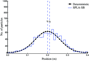
Figure 1: Particle distributions at $t\!=\!2$ s for pure diffusion of a 1000 particle $\delta$ spike obtained using the SPLA and Eq. (27). The initial delta function is shown as a dashed line. The cross-sectional area $A$ is set such that the total concentration over the domain is $0.04~{}M$. The SPLA simulation was performed using the SB-$a_{\mu}$ $\tau$-selection procedure of Table 2 (SPLA-SB).

In Fig. 2, we present a computational cost analysis comparing the SPLA to the NSM. In Fig. 2(a), we see that the SPLA, using both the reaction-based (SPLA-RB) and species-based (SPLA-SB) $\tau$-selection procedures of Tables 1 and 2, requires almost exactly the same number of simulation steps as the NSM up to about 1000 total particles. Beyond that, we see a significant difference between the methods, with the cost of the SPLA decreasing with increasing number of particles and that of the NSM continuing to increase linearly. The reason why the two SPLA methods coincide exactly is because we model diffusion as a first-order elementary process [Eq. (23)]. Thus, the constraint on $|\Delta a_{l\mu}(t)|$ used in reaction-based $\tau$ selection is identical to that on $|\Delta X_{li}(t)|$ used in species-based $\tau$ selection.

In Fig. 2(b), we compare the CPU times for each of the three methods. Here, we see that up to about 1000 total particles the NSM is actually the least expensive of the methods. The SPLA-SB is close behind, however, being slightly less efficient because of the computational overhead associated with $\tau$ selection. Beyond 1000 total particles, we see that the SPLA decreases in computational cost while the cost of the NSM continues to increase linearly. Interestingly, SPLA-RB is significantly less efficient than the SPLA-SB, despite the fact that both methods take the exact same number of steps on average. This is due to two factors: (i) the total number of $\tau^{\mathrm{leap}}$ calculations required in reaction-based $\tau$-selection ($M_{l}\!+\!N_{l}\Gamma_{l}\!=\!78$) as compared to species-based ($N_{l}\!=40$), and (ii) the extra expense associated with calculating rate derivatives in RB $\tau$-selection [Eqn. 15]. Since $N_{l}$ will often be much less than $M_{l}\!+\!N_{l}\Gamma_{l}$, we see that there is a distinct advantage to using SB $\tau$-selection in spatial leaping simulations.

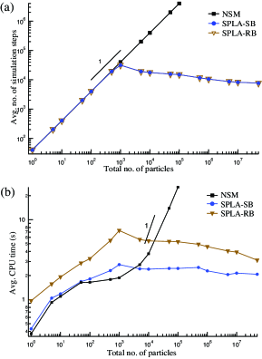
Figure 2: (a) Average numbers of simulation steps and (b) average CPU times vs. total particle number for pure diffusion of a $\delta$ function till $t\!=\!2$ s using the SPLA-RB, SPLA-SB and NSM. In each case, the particle number was changed by varying the cross-sectional area $A$, while maintaining a constant concentration of $0.04~{}M$ over the domain. All results are averaged over 500 simulation runs performed on an Intel Core 2 Duo, 2.13 GHz machine with 2 GB of RAM.

In Fig. 3, we compare the accuracy of the SPLA-SB to the NSM for an initial $\delta$ spike of $10^{4}$ particles. We omit the SPLA-RB since the results are identical to the SPLA-SB. We see that, although the SPLA requires about an order of magnitude fewer steps [Fig. 2(a)], there is essentially no difference between the means and standard deviations obtained from both methods over the entirety of the domain. We make sense of this by referring to the works of Cao et al. Cao04 and Rathinam et al. Rath05 , both of which show that in explicit $\tau$-leaping methods (like SPLA), for sufficiently small $\tau$, the histograms generated using a $\tau$-leaping method should be virtually indistinguishable from those obtained using an exact-stochastic method. Our results in Fig. 3 thus simply indicate that we are using a small enough error control parameter ($\epsilon\!=\!0.01$) in $\tau$ selection and thus avoiding any noticeable errors.

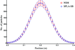
Figure 3: Means and standard deviations of the particle number over the entire domain at $t\!=\!2$ s for pure diffusion of a $10^{4}$ particle $\delta$ function using the SPLA-SB and the NSM. In both cases, results are from 500 simulation runs. The dotted lines constitute an envelope of twice the standard deviation about the SPLA-SB mean.

IV.2 Fisher’s equation

Fisher’s equation (also known as the Fisher-Kolmogorov-Petrovskii-Piscounov equation) Fisher:1937 ; Kolmogorov:1937 is a deterministic partial differential equation that has been used to describe the propagation of an advantageous gene in a population Fisher:1937 and the spatio-temporal evolution of a species under the combined effects of diffusion and logistical growth Kolmogorov:1937 . In one dimension, the equation is of the form

$$\frac{\partial u}{\partial t}=Ku(\bar{c}-u)+D\frac{\partial^{2}u}{\partial y^{2}},$$ (28)

where $u$ is a species concentration, $K$ is a second-order reaction rate constant, $\bar{c}$ is the “carrying capacity” or “saturation value” of the system and $D$ is a diffusion coefficient.

We again consider a one-dimensional domain of width 0.4 m and cross-sectional area $A$ and divide it into $L\!=\!40$ equally-sized subvolumes ($\omega_{l}\!=\!0.01A$ m³) with Neumann (no flux) boundary conditions applied at each end. On this domain, we consider the reaction-diffusion system

$$S_{l1} +S_{l2}\xrightarrow{k}2S_{l1}, l\in\{1{\ldots}L\},$$

$$S_{l1} \xrightleftharpoons[d]{d}S_{(l+1)1}, l\in\{1{\ldots}L-1\},$$ (29)

$$S_{l2} \xrightleftharpoons[d]{d}S_{(l+1)2}, l\in\{1{\ldots}L-1\}.$$

Because $S_{1}$ and $S_{2}$ have equal diffusivities throughout the domain, in the deterministic limit the total population within each subvolume $X_{lT}\!=\!X_{l1}(t)\!+\!X_{l2}(t)$ is constant. The spatio-temporal evolution of $S_{1}$ can thus be described by Fisher’s equation (28) with $d\!=\!D/h^{2}$, $u\!=\!X_{1}(y,t)/\Omega$, $K\!=\!k\Omega$, $\bar{c}\!=\!X_{lT}/\Omega$, where $\Omega\!=\!N_{A}\omega_{l}$ and $N_{A}$ is Avogadro’s number.

Initially, we take the first compartment to be saturated with $S_{1}$ [i.e, $X_{11}(0)\!=\!\bar{c}\Omega$; see Fig. 4] and all other compartments to be saturated with $S_{2}$. The saturation value $\bar{c}$ is taken be $10^{-4}~{}M$ and we choose $D\!=\!10^{-4}$ m²/s and $K\!=\!7\!\times\!10^{4}~{}M^{-1}$ s^-1. To investigate the effects of stochasticity, we hold $\bar{c}$ constant and vary the particle number $X_{lT}$ by varying the cross-sectional area $A$. In Fig. 4, we show a snapshot of the traveling wave of $S_{1}$ obtained by solving Fisher’s equation (28) and the corresponding reaction-diffusion system (29).

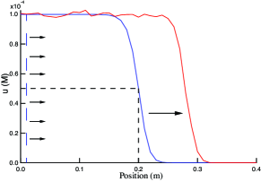
Figure 4: Solution of the one-dimensional Fisher’s equation (28). The initial condition is shown by the dashed lines. The deterministic trajectory (blue) is shown at $t\!=\!3.73$ s, the time at which the solution reaches half its saturation value at $y\!=\!0.2$ m. A stochastic trajectory (red) is shown at $t\!=\!5.0$ s

In Fig. 5, we show a computational cost analysis comparing different variants of the SPLA-SB to the NSM and Marquez-Lago’s and Rossinelli’s spatial $\tau$-leaping methods. [We do not consider the SPLA-RB since it is significantly less efficient than the SPLA-SB]. Simulations are run until $t\!=\!25$ s, and the results are averaged over 500 runs. In Fig. 5(a), we see that, at low populations, the numbers of simulation steps for all methods scale linearly with the number of particles, although the Rossinelli method and SPLA-(no ES events) take an order of magnitude fewer steps. This indicates that these methods are firing multiple events even when the populations are small. Above about $X_{lT}\!=\!100$, however, we see a divergence from the linear trend for all of the leaping methods. The cost of the Marquez-Lago and Rossinelli methods are independent of system size above this point, while that for the full SPLA drops initially, but then continues to increase linearly beyond about $X_{lT}\!=\!500$. However, when we selectively disable the exact-stochastic classification for reactions only in the SPLA we see that the cost decreases significantly, approaching those of Marquez-Lago and Rossinelli. This indicates that, for this system, reaction events are causing a classification cascade at large populations just as diffusion events did in our initial studies. This exemplifies the need to develop a more generalized approach for handling the classification cascade problem (see Sec. III.4). In Fig. 5(b), we see similar trends for the CPU times, although Marquez-Lago’s method and the SPLA are somewhat more costly than the NSM at small populations because of the added overhead associated with $\tau$ selection.

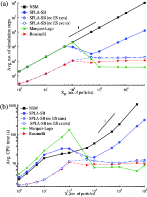
Figure 5: (a) Average numbers of simulation steps and (b) average CPU times vs. $X_{lT}$ for simulations till $t\!=\!25$ s of the reaction-diffusion system (29) using various methods. In each case, the particle number is changed by varying the cross-sectional area $A$ while maintaining a constant concentration of $\bar{c}$ within each $V_{l}$. All results are averaged over 500 simulation runs performed on an Intel Core 2 Duo, 2.13 GHz machine with 2 GB of RAM.

The results in Fig. 5 would seem to indicate that the SPLA is always slower than both the Marquez-Lago and Rossinelli methods. However, this is not entirely true. In Fig. 6, we show the time steps taken during representative simulation runs with $X_{lT}\!=\!10^{4}$ for the various methods. We see that during the first $\sim\!7$ s, when the wave is propagating across the domain, the time steps for the SPLA are small. Rossinelli’s method takes slightly larger time steps during this period while Marquez-Lago’s time steps are significantly larger. The scatter of particularly small time steps for the full SPLA exemplifies the classification cascade effect evident in Fig. 5. We also see how forbidding the exact-stochastic classification for reactions prevents this from occurring. At $\sim\!7$ s, however, the situation changes dramatically. The system approaches equilibrium and the time steps for all leaping methods increase significantly, with Rossinelli’s method experiencing the largest jump, followed by the SPLA and then Marquez-Lago. Also note how the classification cascade problem ceases in the SPLA.

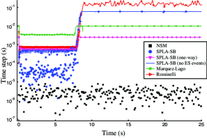
Figure 6: Time steps calculated during individual simulation runs of the reaction-diffusion system (29) with $X_{lT}\!=\!10^{4}$ using various methods.

We make sense of these results by considering the one-way diffusion variant of the SPLA (Sec. III.5), where incoming diffusion is ignored in $\tau$ selection. We see in Fig. 6 that this results in significantly smaller time steps for $t\!\gtrsim\!7$ s. The time period after $\sim\!7$ s corresponds to the equilibrium state of the system, i.e., it takes $\sim\!7$ s for the wave to travel across the domain. At equilibrium, incoming diffusion replenishes the numbers of particles in subvolumes. Ignoring this causes the algorithm to underestimate the time at which the leap condition Eq. (7) will be violated. This explains why the time steps for Marquez-Lago’s method are smaller during this phase than other leaping methods and, if we were to run the simulations longer than $25$ s, SPLA would become more efficient. The remaining disparity between Marquez-Lago and the one-way SPLA is due to differences in $\tau$-selection procedure. The larger time steps for Rossinelli during this phase are due to their separate consideration of reaction and diffusion events.

We find that the different time steps obtained by various methods give rise to different traveling wave velocities $\mathcal{V}$, which we can use to compare the accuracies of the various methods. We measure the velocity as the time taken for $S_{1}$ to reach half its saturation value at $y\!=\!0.2$ m. For the Heaviside initial condition, the analytical expression for the wave velocity is $\mathcal{V}\!=\!2\sqrt{DK\bar{c}}$ Mai:2000 . However, stochastic effects give rise to a distribution of wave velocities for the same initial condition. Recent authors have shown that, depending on the values of $\bar{c}$ and $K$, the mean of the velocity distribution can differ from the analytical velocity Lemarchand:1995 ; Mai:1998 ; Panja:2004 , particularly at low populations. Thus, instead of the analytical solution, we use the mean velocity $\left\langle\mathcal{V}\right\rangle_{\mathrm{NSM}}$ obtained from $500$ NSM simulations as the standard for comparison. In Fig. 7, we show percent deviations between the mean wave velocities obtained from the various leaping methods and $\left\langle\mathcal{V}\right\rangle_{\mathrm{NSM}}$ as a function of $X_{lT}$. In the inset, we show the convergence of $\left\langle\mathcal{V}\right\rangle_{\mathrm{NSM}}$ to the analytical solution with increasing number of particles.

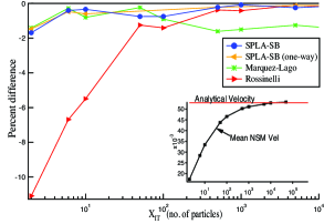
Figure 7: Percent deviations between mean wave velocities obtained from various leaping methods and the NSM for varying system sizes ($\left\langle\mathcal{V}\right\rangle_{\mathrm{leap}}\!-\!\left\langle\mathcal{V}\right\rangle_{\mathrm{NSM}}/\left\langle\mathcal{V}\right\rangle_{\mathrm{NSM}}\!\times\!100\%$). (Inset) Convergence of $\left\langle\mathcal{V}\right\rangle_{\mathrm{NSM}}$ to the analytical solution $\mathcal{V}\!=\!2\sqrt{DK\bar{c}}$ Mai:2000 with increasing system size. All results are based on 500 leaping and NSM simulation runs. Note that the apparent discrepancies between the NSM and the SPLA and Marquez-Lago methods at small particle numbers are simply due to random sampling error [also see Fig. 8(c)].

Fig. 7 shows that, for small populations, Rossinelli’s method has large errors in its wave velocity. The error decreases with increasing population and becomes negligible at the largest system sizes considered. Marquez-Lago’s method, on the other hand, shows the opposite trend: the error is negligible at small populations and increases with increasing population. We can explain these observations by referring back to Figs. 5 and 6. The error in Rossinelli at small populations is mainly due to the fact that the method lacks a mechanism for transitioning to a SSA method. Thus, the increase in efficiency seen in Fig. 5 comes at the cost of accuracy. The error in Marquez-Lago’s method is due to the combined effect of the $\tau$-selection procedure and neglecting incoming diffusion. At small populations, the method transitions to NSM, thus reducing error. At large populations, however, the method takes larger time steps than the other leaping methods during the wave-propagation phase (Fig. 6), resulting in the increased error seen in Fig. 7. Furthermore, in the equilibrium phase (after $\sim\!7$ s), the method takes smaller steps than SPLA and the error then changes from one of accuracy to one of efficiency. SPLA addresses each of these issues and shows negligible error over the entire population range. SPLA-(one way) tries to capture just the effect of neglecting incoming diffusion. However, we do not observe any significant error because the method transitions to an exact-stochastic method at small populations and, calculates leap time steps that are fairly near the accurate SPLA time steps at higher populations.

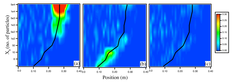
Figure 8: Kolmogorov distances at $t\!=\!5$ s obtained using: (a) Marquez-Lago, (b) Rossinelli, and (c) SPLA. The x-axis corresponds to position within the domain and the y-axis to system size (i.e., $X_{lT}$). All results are based on 500 leaping and NSM simulation runs. The NSM self distance is subtracted from the Kolmogorov distances and negative values are clipped to zero. The black line is the mean position of the wavefront for different system sizes. We can infer from this that the simulation error arises mainly at the propagating wavefront.

While the means of velocities are instructive in providing general insight into the accuracies of the methods, they do not give complete information about the particle distributions over the entire domain. Thus, for a more accurate analysis, we use the Kolmogorov-Smirnov test Cao:2006a , a statistical test used to compare two given distributions. If the particle number distribution for $S_{1}$ within a given subvolume $V_{l}$ at time $t$ is $P(X_{l1}(t))$ for a leaping method and $\widetilde{P}(X_{l1}(t))$ for the NSM, then the Kolmogorov distance between the two distributions is defined as $\mathcal{K}(X_{l1}(t))\!\equiv\!\max|F(X_{l1}(t))\!-\!\widetilde{F}(X_{l1}(t))|$, where $F(x)\!\equiv\!\int_{-\infty}^{x}P(x)dx$ is the cumulative distribution function of $P(x)$. The reference distribution $\widetilde{P}(X_{l1}(t))$ is also associated with a “self distance” $\mathcal{S}(X_{l1}(t))$ Cao:2006a , which is a measure of the uncertainty associated with building the distribution from a finite set of realizations. Only if $\mathcal{K}(X_{l1}(t))\!>\!\mathcal{S}(X_{l1}(t))$ can we say that the two distributions are statistically distinct.

In Fig. 8, we plot the differences $\mathcal{K}(X_{l1}(5))\!-\!\mathcal{S}(X_{l1}(5))$ over the entire domain $l\!\in\!\{1{\ldots}L\}$ obtained using the full SPLA and the methods of Marquez-Lago and Rossinelli for various values of $X_{lT}$. A positive value of this difference indicates regions where the solution obtained from the various leaping methods differs, in a statistically significant sense, from the NSM. These plots reinforce the observations made above: (i) errors arise in Marquez-Lago at large populations, (ii) errors arise in Rossinelli at small populations, and (iii) the full SPLA is accurate over the entire domain for all system sizes considered. Moreover, we see that the errors in Figs. 8(a)–(c) arise mainly at the propagating wavefront.

IV.3 Gray-Scott equations

First studied by Pearson Pearson:1993 , the Gray-Scott equations

$$\frac{\partial u}{\partial t} =-uv^{2}+F(1-u)+D_{u}\nabla^{2}u,$$

$$\frac{\partial v}{\partial t} =uv^{2}-(F+k)v+D_{v}\nabla^{2}v,$$ (30)

describe the spatio-temporal behavior of a two-component reaction-diffusion system. The equations are of particular interest because they produce a rich variety of spatio-temporal patterns based on the values of $F$ and $k$. Here, we set $F\!=\!0.035$, $k\!=\!0.060$, $D_{u}\!=\!2{\times}10^{-5}$ m²/s and $D_{v}\!=\!10^{-5}$ m²/s.

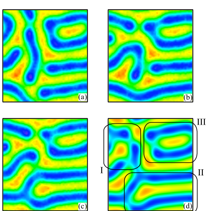
Figure 9: Snapshots of the Gray-Scott reaction-diffusion system (31) at $t\!=\!1500$ s obtained using (a) Marquez-Lago, (b) Rossinelli, (c) the full SPLA-SB, and (d) Eqs. (30). The concentration of $S_{1}$ (plotted above) ranges from 0 (blue) to 1 (red) $M$. The features present in regions I, II and III are compared for different simulation methods. All simulations are performed with the parameters $F\!=\!0.035$, $k\!=\!0.060$, $D_{u}\!=\!2{\times}10^{-5}$ m²/s and $D_{v}\!=\!10^{-5}$ m²/s.

We consider a two-dimensional domain of width 0.5 m and length 0.5 m (in say, the y-z plane) and height $H$ and divide it into a regular $50{\times}50$ grid ($L\!=\!2500$; $\omega_{l}\!=\!0.25H$ m³, $\Omega\!=\!N_{A}\omega_{l}$) with periodic boundary conditions. On this domain, we consider the two-component reaction-diffusion system

$$S_{l1} +2S_{l2}\xrightarrow{k_{1}}3S_{l2}, l\in\{1{\ldots}L\},$$

$$S_{l1} \xrightleftharpoons[k_{-2}]{k_{2}}\emptyset, l\in\{1{\ldots}L\},$$

$$S_{l2} \xrightarrow{k_{3}}\emptyset, l\in\{1{\ldots}L\},$$ (31)

$$S_{l1} \xrightleftharpoons[d_{1}]{d_{1}}S_{l^{\prime}1}, l\in\{1{\ldots}L\}, l^{\prime}\in\mathbf{C}_{l},$$

$$S_{l2} \xrightleftharpoons[d_{2}]{d_{2}}S_{l^{\prime}2}, l\in\{1{\ldots}L\}, l^{\prime}\in\mathbf{C}_{l}.$$

If we set the parameters $k_{1}\!=\!1/\Omega^{2}$ s^-1, $k_{2}\!=\!F$ s^-1, $k_{-2}\!=\!F\Omega$ s^-1 and $k_{3}\!=\!F\!+\!k$ s^-1, then in the deterministic limit the spatio-temporal evolutions of $S_{1}$ and $S_{2}$ are described by the Gray-Scott equations (30) with $u\!=\!X_{1}(y,z,t)/\Omega$, $v\!=\!X_{2}(y,z,t)/\Omega$, $d_{1}\!=\!D_{u}/h^{2}$ and $d_{2}\!=\!D_{v}/h^{2}$.

In the deterministic case, a unique pattern is obtained from Eqs. (30) for a given set of parameters $\{F,k,D_{u},D_{v}\}$ and initial conditions Pearson:1993 . However, the pattern formation behavior can change significantly in the presence of noise Lesmes:2003 , to the extent that large amounts of internal noise can prevent pattern formation altogether Wang:2007b . We investigate the effects of noise in the Gray-Scott system by performing stochastic simulations using the SPLA-SB, Marquez-Lago and Rossinelli methods, but we consciously choose conditions that minimize stochastic effects so that direct comparisons can be made to the deterministic solution.

Initially, we set the concentration of $S_{1}$ and $S_{2}$ in each subvolume to $1~{}M$ and $0.1~{}M$ respectively and choose $H$ such that $1~{}M$ corresponds to to 5000 particles. We then apply a perturbation that triggers pattern formation in the reaction diffusion system. In Fig. 9, we show snapshots of the patterns obtained from the different simulations methods and from the solution of Eqs. (30) at $t\!=\!1500$ s.

By comparing Figs. 9(a)–(c) to Fig. 9(d), the effects of noise are visually evident. Rather than the smooth pattern produced in the deterministic case, those obtained from the leaping methods have clear fluctuations. The effects are small, however, and all of the patterns are superficially similar, although close inspection reveals perceptible differences. We highlight three regions (I, II and III) in the deterministic solution of Fig. 9 to make visual comparison of the patterns easier. The pitchfork-type pattern in region II is present in SPLA and to some extent in Rossinelli’s method. That feature is barely recognizable Marquez-Lago’s method. Similarly in region I, SPLA’s pattern is the closer to the deterministic solution than other methods. However, the patterns present in region III are similar in all the simulation methods. From this we argue that the SPLA pattern in Fig. 9(c) is most similar to the deterministic solution in Fig. 9(d) and that the Marquez-Lago pattern in Fig. 9(a) is most dissimilar. Since we consciously aimed to minimize the effects of stochasticity in the pattern formation, these results imply that the most faithful description of the system dynamics is given by the SPLA.

In order to ascertain why this is, we compare the time steps taken by the SPLA to those for the Marquez-Lago and Rossinelli methods. The main result (plot not shown) is that the full SPLA generally takes smaller time steps than the other methods, explaining why it gives more accurate results.

It is important to note that our analysis of the Gray-Scott system is limited due to the large number of total events in the system. With 2500 subvolumes, each with four nearest neighbors, there are a total of $10^{4}$ reactions and $2{\times}10^{4}$ diffusion events that must be taken into account. As such, a single SPLA simulation of 1500 s took $1.43$ h to complete. Marquez-Lago and Rossinelli simulations took a comparable amount of time ($0.36$ h and, $0.92$ h respectively). This is an important result because it exemplifies a serious shortcoming of the spatial $\tau$-leaping approach in general. Although leaping is beneficial in allowing multiple event firings at each simulation step, the high cost of $\tau$ selection severely limits the applicability of the approach in the face of large event numbers, as is common in spatially-discretized systems. Thus, in order to make the approach practicable, improving the efficiency of the method is of paramount importance. We discuss this issue in more detail in Sec. V.

V Discussion and Conclusion

We have presented the spatial partitioned-leaping algorithm as an accurate formulation of the leaping approach for reaction-diffusion systems on discretized grids. Our primary contributions have been to correctly enumerate all of the events that must be considered during the time-step calculation process and to recast the reaction-based and species-based $\tau$-selection formulas Cao06:newStep ; Harris06 within a spatial context (Tables 1 and 2). The main differences between these formulas and those used in prior implementations of spatial $\tau$-leaping Lago07 ; Rossi08 are that reaction and diffusion events are considered together and the effects of incoming diffusion are properly taken into account. Both aspects are crucial for an accurate spatial leaping implementation and we have shown, through numerical examples, how improper consideration can lead to the introduction of error or a reduction in efficiency, depending on the specifics of the system being studied. We have also shown the implications, in terms of accuracy, of not providing a mechanism for transitioning to a exact-stochastic method in the limit of small populations.

Furthermore, we have shown that the species-based $\tau$-selection procedure, besides being inherently less costly per calculation than the reaction-based procedure (because of the lack of rate derivatives Cao06:newStep ), will generally require far fewer total calculations for spatial systems than the reaction-based approach. This is because the total number of events in a discretized system will often far exceed the total number of species. Species-based $\tau$-selection will thus be the preferred choice in most situations. Exceptions include cases where rate constants are time dependent, e.g., if environmental quantities such as temperature and volume vary in time (species-based $\tau$-selection assumes time-invariant rate constants). In such situations, modified forms of the reaction-based $\tau$-selection formulas will be required.

Inclusion of the exact-stochastic classification in the algorithm brings along problems of classification cascade, induced by events at the edge of diffusing fronts, which eventually results in an unnecessarily small time step and, hence, a significant reduction in efficiency. This phenomenon has been observed previously for a well-mixed biochemical system involving binding of transcription factors to individual genes Harris09 and is a shortcoming of the PLA in general. Here, we have attenuated this problem to an extent by restricting the classification of diffusion events as exact-stochastic when the population of the diffusing species exceeds a pre-specified threshold (i.e., 100). This approach is ad hoc, however, and we have demonstrated the need to develop a more general approach that can handle all cases. Work is currently underway in this direction.

A shortcoming of the SPLA, and other spatial leaping methods in general, is the strong dependence of the computational cost on the total number of events in the system. This is a well-known problem for stochastic simulation algorithms Petti05 and is exemplified by the large amount of time taken to analyze the moderately complex Gray-Scott system (involving $3\!\times\!10^{4}$ unique events involving 5000 unique species). These methods remain constrained by the fact that one $\tau$-selection calculation must ultimately be performed for each event (reaction-based) or species (species-based) present in the system. In order to make the approach practicable, a solution to this problem is clearly required. A computational approach can be to parallelize the algorithm, parsing out the computational effort across multiple machines. Many aspects of the SPLA are indeed parallel in nature, such as $\tau$ selection, event classification and event update. From an algorithmic perspective, Anderson’s post-leap checking procedure Ander08 may provide some relief in that it obviates the need to perform the expensive pre-leap calculations. Pettigrew and Resat Petti07 have proposed an approximate post-leap checking procedure that might prove useful as well.

Another possibility is to fundamentally reduce the number of $\tau$ selection calculations by performing them on groups of events rather than on individual events or species. The challenge, however, is that in contrast to the exact-stochastic case (Sec. II.1.2), it is not permissible within the context of a leaping algorithm to group arbitrary sets of events and then perform $\tau$ selection on the group. This is because the leap condition Eq. (7) applies at the level of individual events, not groups. Basically, there is no guarantee that a given change in the summed propensity of the group will translate into equivalent changes in the propensities of the events that comprise the group. However, it may be possible to identify special types of groups in which this is, in fact, the case. This type of grouping, based on event type rather than on location, is fundamentally different from that used in typical spatial simulation methods. It also differs from the type of grouping used in the multinomial $\tau$-leaping method of Pettigrew and Resat Petti07 , a well-known binomial $\tau$-leaping variant. We are actively pursuing this avenue of research.

Compounding the problem of exact-stochastic event classifications is that SPLA transitions to NRM, which is an inefficient exact-stochastic method for spatial simulations. Ideally, the method would segue to an efficient spatial SSA formulation such as the NSM. However, the NSM, which is based on grouping events by subvolume, does not fit naturally into the framework of the SPLA for the reasons cited above, i.e., $\tau$ selection cannot be applied at the level of groups. Marquez-Lago incorporate the NSM into their spatial $\tau$-leaping method by classifying subvolumes as exact-stochastic if $a_{l0}(t)\!\lesssim\!10$ (Sec. III.5), emulating the approach taken by Gillespie, Petzold and co-workers Gillesp01 ; Gillesp03 ; Cao06:newStep . We could employ a similar approach in the SPLA. However, it is our hope that a more natural method of transition will arise from our attempts to incorporate grouping generally into the leaping methodology.

Our development of the SPLA is significant in that it represents a “gold standard” in terms of accuracy against which future enhancements and extensions to the spatial $\tau$-leaping approach can be compared. As a straightforward implementation of spatial leaping, the method is not maximally optimized in terms of efficiency nor is it meant to be. However, it does achieve the maximum possible gains in efficiency for a method that accurately employs pre-leap $\tau$ selection at the level of individual events by considering only those events that are of consequence to the calculation. These include local reactions and outgoing and incoming diffusion events to and from neighboring subvolumes. We hope that future innovations addressing the challenges highlighted here will help to further improve the leaping methodology and make stochastic simulations of complex systems practicable.

VI Acknowledgments

We thank the anonymous reviewers for their useful inputs and the Semiconductor Research Corporation for financial support.

References

- (1) A. P. Arkin, J. Ross, and H. H. McAdams. Stochastic kinetic analysis of developmental pathway bifurcation in phage -infected Escherichia coli cells. Genetics, 149:1633–1648, 1998.
- (2) H. H. McAdams and A. Arkin. It’s a noisy business! genetic regulation at the nanomolar scale. Trends Genet., 15:65, 1999.
- (3) M. B. Elowitz, A. J. Levine, E. D. Siggia, and P. S. Swain. Stochastic gene expression in a single cell. Science, 297:1183–1186, 2002.
- (4) N. Fedoroff and W. Fontana. Small numbers of big molecules. Science, 297:1129–1131, 2002.
- (5) C. V. Rao, D. M. Wolf, and A. P. Arkin. Control, exploitation and tolerance of intracellular noise. Nature, 420:231–237, 2002.
- (6) D. Longo and J. Hasty. Dynamics of single-cell gene expression. Mol. Syst. Biol., 28 November 2006. doi:10.1038/msb4100110.
- (7) M. S. Samoilov, G. Price, and A. P. Arkin. From fluctuations to phenotypes: The physiology of noise. Sci. STKE, 2006 (366):re17, 2006.
- (8) J. D. Plummer and P. B. Griffin. Challenges for predictive process simulation in sub 0.1 m silicon devices. Nucl. Instr. Meth. Phys. Res. B, 102:160, 1995.
- (9) S. Roy and A. Asenov. Where do the dopants go? Science, 309:388, 2005.
- (10) V. Johánek, M. Laurin, A. W. Grant, B. Kasemo, C. R. Henry, and J. Libuda. Fluctuations and bistabilities on catalyst nanoparticles. Science, 304:1639–1644, 2004.
- (11) D. T. Gillespie. A general method for numerically simulating the stochastic time evolution of coupled chemical reactions. J. Comput. Phys., 22:403–434, 1976.
- (12) D. T. Gillespie. Exact stochastic simulation of coupled chemical reactions. J. Phys. Chem., 81:2340–2361, 1977.
- (13) D. T. Gillespie. Stochastic simulation of chemical kinetics. Annu. Rev. Phys. Chem., 58:35–55, 2007.
- (14) D. Endy and R. Brent. Modelling cellular behaviour. Nature, 409:391–395, 2001.
- (15) D. T. Gillespie. Approximate accelerated stochastic simulation of chemically reacting systems. J. Chem. Phys., 115:1716–1733, 2001.
- (16) D. T. Gillespie and L. R. Petzold. Improved leap-size selection for accelerated stochastic simulation. J. Chem. Phys., 119:8229–8234, 2003.
- (17) M. Rathinam, L. R. Petzold, Y. Cao, and D. T. Gillespie. Stiffness in stochastic chemically reacting systems: The implicit tau-leaping method. J. Chem. Phys., 119:12784–12794, 2003.
- (18) Y. Cao, D. T. Gillespie, and L. R. Petzold. Avoiding negative populations in explicit Poisson tau-leaping. J. Chem. Phys., 123:054104, 2005.
- (19) Y. Cao, D. T. Gillespie, and L. R. Petzold. Efficient step size selection for the tau-leaping method. J. Chem. Phys., 124:044109, 2006.
- (20) Y. Cao, D. T. Gillespie, and L. R. Petzold. Adaptive explicit-implicit tau-leaping method with automatic tau selection. J. Chem. Phys., 126:224101, 2007.
- (21) T. Tian and K. Burrage. Binomial leap methods for simulating stochastic chemical kinetics. J. Chem. Phys., 121:10356–10364, 2004.
- (22) A. Chatterjee, D. G. Vlachos, and M. A. Katsoulakis. Binomial distribution based -leap accelerated stochastic simulation. J. Chem. Phys., 122:024112, 2005.
- (23) A. Auger, P. Chatelain, and P. Koumoutsakos. R-leaping: Accelerating the stochastic simulation algorithm by reaction leaps. J. Chem. Phys., 125:084103, 2006.
- (24) X. Cai and Z. Xu. K-leap method for accelerating stochastic simulation of coupled chemical reactions. J. Chem. Phys., 126:074102, 2007.
- (25) M. F. Pettigrew and H. Resat. Multinomial tau-leaping method for stochastic kinetic simulations. J. Chem. Phys., 126:084101, 2007.
- (26) X. Peng, W. Zhou, and Y. Wang. Efficient binomial leap method for simulating chemical kinetics. J. Chem. Phys., 126:224109, 2007.
- (27) M. Rathinam and H. El Samad. Reversible-equivalent-monomolecular tau: A leaping method for “small number and stiff” stochastic chemical systems. J. Comput. Phys., 224:897–923, 2007.
- (28) D. F. Anderson. Incorporating postleap checks in tau-leaping. J. Chem. Phys., 128:054103, 2008.
- (29) Z. Xu and X. Cai. Unbiased -leap methods for stochastic simulation of chemically reacting systems. J. Chem. Phys., 128:154112, 2008.
- (30) A. Leier, T. T. Marquez-Lago, and K. Burrage. Generalized binomial -leap method for biochemical kinetics incorporating both delay and intrinsic noise. J. Chem. Phys., 128:205107, 2008.
- (31) L. A. Harris and P. Clancy. A “partitioned leaping” approach for multiscale modeling of chemical reaction dynamics. J. Chem. Phys., 125:144107, 2006.
- (32) L. Trinkle-Mulcahy and A. I. Lamond. Nuclear functions in space and time: Gene expression in a dynamic, constrained environment. FEBS Lett., 582:1960–1970, 2008.
- (33) E. Callaway. Bacteria’s new bones. Nature, 451:124–126, 2008.
- (34) R. J. Ellis. Macromolecular crowding: obvious but underappreciated. Trends Biochem. Sci., 26:597–604, 2001.
- (35) H.-X. Zhou, G. Rivas, and A. P. Minton. Macromolecular crowding and confinement: Biochemical, biophysical, and potential physiological consequences. Annu. Rev. Biophys., 37:375–397, 2008.
- (36) T. S. Shimizu, S. V. Aksenov, and D. Bray. A spatially extended stochastic model of the bacterial chemotaxis signalling pathway. J. Mol. Biol., 329:291–309, 2003.
- (37) J. V. Rodríguez, J. A. Kaandorp, M. Dobrzyński, and J. G. Blom. Spatial stochastic modelling of the phosphoenolpyruvate-dependent phosphotransferase (pts) pathway in Escherichia coli. Bioinformatics, 22:1895–1901, 2006.
- (38) T. Fricke and D. Wendt. The markoff automaton: A new algorithm for simulating the time-evolution of large stochastic dynamic systems. Int. J. Mod. Phys. C, 6:277–306, 1995.
- (39) M. E. Gracheva, R. Toral, and J. D. Gunton. Stochastic effects in intercellular calcium spiking in hepatocytes. J. Theor. Biol., 212:111–125, 2001.
- (40) J. Elf and M. Ehrenberg. Spontaneous separation of bi-stable biochemical systems into spatial domains of opposite phases. IEE Syst. Biol., 1:230–236, 2004.
- (41) J. Hattne, D. Fange, and J. Elf. Stochastic reaction-diffusion simulation with MesoRD. Bioinformatics, 21:2923–2924, 2005.
- (42) D. Bernstein. Simulating mesoscopic reaction-diffusion systems using the Gillespie algorithm. Phys. Rev. E, 71:041103, 2005.
- (43) K. Takahashi, S. N. V. Arjunan, and M. Tomita. Space in systems biology of signaling pathways—towards intracellular molecular crowding in silico. FEBS Lett., 579:1783–1788, 2005.
- (44) C. Lemerle, B. Di Ventura, and L. Serrano. Space as the final frontier in stochastic simulations of biological systems. FEBS Lett., 579:1789–1794, 2005.
- (45) S. S. Andrews and A. P. Arkin. Simulating cell biology. Curr. Biol., 16:R523–R527, 2006.
- (46) M. Dobrzyński, J. V. Rodríguez, J. A. Kaandorp, and J. G. Blom. Computational methods for diffusion-influenced biochemical reactions. Bioinformatics, 23:1969–1977, 2007.
- (47) A. Chatterjee and D. G. Vlachos. An overview of spatial microscopic and accelerated kinetic Monte Carlo methods. J. Computer-Aided Mater. Des., 14:253–308, 2007.
- (48) T. T. Marquez-Lago and K. Burrage. Binomial tau-leap spatial stochastic simulation algorithm for applications in chemical kinetics. J. Chem. Phys., 127:104101, 2007.
- (49) D. Rossinelli, B. Bayati, and P. Koumoutsakos. Accelerated stochastic and hybrid methods for spatial simulations of reaction-diffusion systems. Chem. Phys. Lett., 451:136–140, 2008.
- (50) Throughout this article, we will use the indices and when referring to events (reaction and diffusion), and when referring to species and and for subvolumes.
- (51) M. A. Gibson and J. Bruck. Efficient exact stochastic simulation of chemical systems with many species and many channels. J. Phys. Chem. A, 104:1876–1889, 2000.
- (52) A. Slepoy, A. P. Thompson, and S. J. Plimpton. A constant-time kinetic Monte Carlo algorithm for simulation of large biochemical reaction networks. J. Chem. Phys., 128:205101, 2008.
- (53) T. P. Schulze. Efficient kinetic Monte Carlo simulation. J. Comput. Phys., 227:2455–2462, 2008.
- (54) Jurgen Pahle. Biochemical simulations: stochastic, approximate stochastic and hybrid approaches. Brief. Bioinform., 10(1):53–64, 2009.
- (55) D. T. Gillespie. The chemical langevin equation. J. Chem. Phys., 113:297–306, 2000.
- (56) L. A. Harris, A. M. Piccirilli, E. R. Majusiak, and P. Clancy. Quantifying stochastic effects in biochemical reaction networks using partitioned leaping. Phys. Rev. E, 79:051906, 2009.
- (57) W. H. Press, S. A. Teukolsky, W. T. Vetterling, and B. P. Flannery. Numerical Recipes in C, The Art of Scientific Computing, 2nd Ed. Cambridge University Press, New York, NY, 1999. Standard techniques for generating Poisson and normal random deviates.
- (58) R. A. Fisher. The wave of advance of advantageous genes. Ann. Eugenics, 7:355–369, 1937.
- (59) A. Kolmogorov, I. Petrovskii, and N. Piscounov. A study of the diffusion equation with increase in the amount of substance, and its application to a biological problem. In Selected Works of A. N. Kolmogorov I, pages 248–270. Kluwer, 1991.
- (60) J. E. Pearson. Complex patterns in a simple system. Science, 261(5118):189–192, 1993.
- (61) Yang Cao, Linda R. Petzold, Muruhan Rathinam, and Daniel T. Gillespie. The numerical stability of leaping methods for stochastic simulation of chemically reacting systems. The Journal of Chemical Physics, 121(24):12169–12178, 2004.
- (62) Muruhan Rathinam, Linda R. Petzold, Yang Cao, and Daniel T. Gillespie. Consistency and stability of tau-leaping schemes for chemical reaction systems. Multiscale Modeling & Simulation, 4(3):867–895, 2005.
- (63) J. Mai, I. M. Sokolov, and A. Blumen. Front propagation in one-dimensional autocatalytic reactions: The breakdown of the classical picture at small particle concentrations. Phys. Rev. E, 62(1):141–145, Jul 2000.
- (64) A. Lemarchand, A. Lesne, and M. Mareschal. Langevin approach to a chemical wave front: Selection of the propagation velocity in the presence of internal noise. Phys. Rev. E, 51(5), 1995.
- (65) J. Mai, I. M. Sokolov, and A. Blumen. Discreteness effects on the front propagation in the reaction in 3 dimensions. Europhys. Lett., 44(1):7–12, 1998.
- (66) D. Panja. Effects of fluctuations on propagating fronts. Phys. Rep., 393(2):87–174, 2004.
- (67) Y. Cao and L. Petzold. Accuracy limitations and the measurement of errors in the stochastic simulation of chemically reacting systems. J. Comput. Phys., 212(1):6–24, 2006.
- (68) F. Lesmes, D. Hochberg, F. Morán, and J. Pérez-Mercader. Noise-controlled self-replicating patterns. Phys. Rev. Lett., 91(23):238301, Dec 2003.
- (69) H. Wang, Z. Fu, X. Xu, and Q. Ouyang. Pattern formation induced by internal microscopic fluctuations. J. Phys. Chem. A, 111(7):1265–1270, 2007.
- (70) Michel F. Pettigrew and Haluk Resat. Modeling signal transduction networks: A comparison of two stochastic kinetic simulation algorithms. The Journal of Chemical Physics, 123(11):114707, 2005.