First Order Quark-Hadron Phase Transition in the NJL-Type Nuclear and Quark Model

Abstract

The quark-hadron phase transition at finite baryon chemical potential is investigated in the extended Nambu-Jona-Lasinio model in which the scalar-vector eight-point interaction is included holding the chiral symmetry. By comparing a pressure of the symmetric nuclear matter with that of the quark matter, the realized phase at given baryon density is determined. As a result, the first order quark-hadron phase transition is derived where the deconfinement transition occurs after the chiral symmetry restoration in this model.

1 Introduction

One of the recent interests in the systems governed by the quantum chromodynamics (QCD) may be to understand the phase diagram and/or the phase transitions between various phases in the quark-gluon and the hadronic matters. As for the chiral phase transition, many works have been done in the various effective models of QCD at finite temperature and/or density. However, to obtain definite results of the quark-hadron phase transition at finite baryon density is still difficult because of the color confinement on the side of the hadronic phase. Of course, the study based on the lattice QCD is also difficult at finite density at present.

For the symmetric nuclear matter, it is important to describe the property of nuclear saturation. The Walecka model[1] has succeeded in describing the saturation property of symmetric nuclear matter as a relativistic system. The success is mainly due to the cancellation of the large scalar and vector potential which are derived by the $\sigma$ meson and $\omega$ meson exchanges between nucleons, respectively. In this model, the nucleon is treated as not a composit but a fundamental particle. Although this model has given many successful results for nuclei and nuclear matter, this model at first stage has no chiral symmetry which plays an important role in QCD.

The celebrated Nambu-Jona-Lasinio (NJL) model[2] gives many important results for hadronic world[3] based on the concenpts of the chiral symmetry and the dynamical chiral symmetry breaking. This model has been applied to the investigation of the dense quark matter.[4] Also, by using this model, the stability of nuclear matter, as well as quark matter, was investigated in which the nucleon is constructed from the viewpoint of quark-diquark picture.[5] On the other hand, it is known that, if the nucleon field is regarded as a fundamental fermion field, not composite one, the nuclear saturation property can not be reproduced starting from the original NJL Lagrangian. However, if the scalar-vector and isoscalar-vector eight-point interactions are introduced holding the chiral symmetry in the original NJL model, the nuclear saturation property is well reproduced[6] where the nucleon is treated as a fundamental fermion.

In this paper, paying an attention to the chiral symmetry, the NJL-type model is adopted in both the nuclear and quark matters. As for the nuclear matter, we adopt the extended NJL model with the eight-point interactions and regard the nucleon field as a fundamental fermion field with the number of color, $N_{c}$, being one.[7, 8] Also, we adopt the extended NJL model with $N_{c}=3$ for the quark matter. Thus, the quark-hadron phase transition is investigated by using the same-type model with the chiral symmetry for nuclear and quark matters in a unified way, the model parameters and the number of color of which are different. As the first step to invetigate the quark-hadron phase transition, in this paper, we consider the symmetric nuclear matter and free quark phase without quark-pair correlation. Namely, we do not take into account of the color superconducting phase in the quark phase at finite density and at zero temperature.[9] This phase may exist at finite density, but, in this paper, the investigation is rest at future. Also, we only consider the symmetric nuclear matter, while it is interesting to the study of the neutron matter which leads to the understanding of the physics of neutron star.[10]

This paper, is organized as follows: In the next section, we introduce the extended NJL model at finite temperature and baryon chemical potential for nuclear and quark matters. The mean field approximation in this model is given. The derived results are identical to those derived by the minimization of the thermodynamical potential density. In §3, the method to determine the model parameters is presented for nuclear matter and quark matter, respectively. In §4, the numerical results are given. In §5, the quark-hadron phase transition is described in this model. The last section is devoted to a summary and concluding remarks.

2 Extended NJL model for nuclear and quark matter at finite temperature and density

In this section, the same models for the nuclear and quark matters are considered in which parameters are different for nuclear and quark matters. One possibe model may be a Nambu-Jona-Lasinio (NJL) model[2] for nucleons and/or quarks. The NJL model is useful because it implements in a simple way the important chiral symmetry. As for the nuclear matter, the property of nuclear saturation must be realized. Then, as one of the possible models, we give the NJL-type model in which the fermions interact with each other through the original NJL-type four-point intaraction plus four point vector-vector and eight-point scalar-vector and isoscalar-vector interactions. This model is called an extended NJL model in this paper.

2.1 Extended NJL model for nuclear and quark matters at finite density and temperature

In this paper, we start with the following Lagrangian density[7, 6] for nuclear matter ($i=N$) and qurak matter ($i=q$):

$${\cal L}_{i} = {\overline{\psi}}_{i}i\gamma^{\mu}\partial_{\mu}\psi_{i}+G_{s}^{i}(({\overline{\psi}}_{i}{\psi}_{i})^{2}+({\overline{\psi}}_{i}i\gamma_{5}{\mib\tau}\psi_{i})^{2})-G_{v}^{i}({\overline{\psi}}_{i}\gamma^{\mu}\psi_{i})({\overline{\psi}}_{i}\gamma_{\mu}\psi_{i})$$ (1)

$$-G_{sv}^{i}(({\overline{\psi}}_{i}{\psi}_{i})^{2}+({\overline{\psi}}_{i}i\gamma_{5}{\mib\tau}\psi_{i})^{2})({\overline{\psi}}_{i}\gamma^{\mu}\psi_{i})({\overline{\psi}}_{i}\gamma_{\mu}\psi_{i})\ .$$

Here, $\psi_{i}$ represents nucleon field ($i=N$) or quark field ($i=q$). The first two terms give the original NJL Lagrangian density. However, the nuclear matter saturation properties are not reproduced if only these two terms are taken into account. Thus, we introduce other two terms, following Ref.KBKM87. Namely, a vector-vector repulsive term, whose interaction strength is represented by $G_{v}^{i}$, and a vector-scalar coupling term, whose interaction strength is represented by $G_{sv}^{i}$, are introduced. This model is nonrenormalizable. Thus, it is necessary to introduce the cutoff parameter $\Lambda_{i}$. We adopt a three-momentum cutoff scheme.

We apply the mean field approximation to the above Lagrangian density. By mean field approximation we mean that we replace bi-linear quantities in the fermion fields, such as ${\overline{\psi}}\Gamma\psi$, by $\langle{\overline{\psi}}\Gamma\psi\rangle+({\overline{\psi}}\Gamma\psi-\langle{\overline{\psi}}\Gamma\psi\rangle)$, and keep only linear terms in the fluctuation $({\overline{\psi}}\Gamma\psi-\langle{\overline{\psi}}\Gamma\psi\rangle)$. Here, the symbol $\langle\cdots\rangle$ denotes the expectation value or thermal average. Only the expectation values of ${\overline{\psi}}_{i}i\gamma^{\mu}\partial_{\mu}\psi_{i}$ and ${\overline{\psi}}_{i}\psi_{i}$ survive at finite temperature and density. The mean field Lagrangian density ${\cal L}_{i}^{MF}$ and the mean field Hamiltonian density ${\cal H}_{i}^{MF}$ are easily obtained as

$${\cal L}_{i}^{MF} = {\overline{\psi}}_{i}(i\gamma^{\mu}\partial_{\mu}-m_{i})\psi-{\widetilde{\mu}}_{i}{\overline{\psi}}_{i}\gamma^{0}\psi_{i}+C_{i}\ ,$$

$${\cal H}_{i}^{MF} = -i{\overline{\psi}}_{i}{\mib\gamma}\cdot\nabla\psi_{i}+m_{i}{\overline{\psi}}_{i}\psi_{i}+{\widetilde{\mu}}_{i}{\overline{\psi}}_{i}\gamma^{0}\psi_{i}-C_{i}\ ,$$ (2)

$$C_{i}\equiv-G_{s}^{i}\langle\!\langle{\overline{\psi}}_{i}\psi_{i}\rangle\!\rangle^{2}+G_{v}^{i}\langle\!\langle{\overline{\psi}}_{i}\gamma^{0}\psi_{i}\rangle\!\rangle^{2}+G_{sv}^{i}\langle\!\langle{\overline{\psi}}_{i}\psi_{i}\rangle\!\rangle^{2}\langle\!\langle{\overline{\psi}}_{i}\gamma^{0}\psi_{i}\rangle\!\rangle^{2}\ ,$$

where we define $m_{i}$ and ${\widetilde{\mu}}_{i}$ as

$$m_{i}=-2G_{s}^{i}\langle\!\langle{\overline{\psi}}_{i}\psi_{i}\rangle\!\rangle+2G_{sv}^{i}\langle\!\langle{\overline{\psi}}_{i}\psi_{i}\rangle\!\rangle\langle\!\langle{\overline{\psi}}_{i}\gamma^{0}\psi_{i}\rangle\!\rangle^{2}\ ,$$ (3)

$${\widetilde{\mu}}_{i}=2G_{v}^{i}\langle\!\langle{\overline{\psi}}_{i}\gamma^{0}\psi_{i}\rangle\!\rangle+2G_{sv}^{i}\langle\!\langle{\overline{\psi}}_{i}\psi_{i}\rangle\!\rangle^{2}\langle\!\langle{\overline{\psi}}_{i}\gamma^{0}\psi_{i}\rangle\!\rangle\$$ (4)

for the nuclear matter ($i=N$) and the quark matter ($i=q$), respectively. Here, the symbol $\langle\!\langle\cdots\rangle\!\rangle$ denotes the thermal average which is given latter, while in this paper we only treat the zero temperature system. Also, the symbol $\langle\cdots\rangle$ will be used for the expectation values at zero temperature.

We deal with a finite density system in this paper. In order to calculate the physical quantities at finite density, we introduce the chemical potential $\mu_{i}$ :

$${\cal H}_{i}^{\prime} = {\cal H}_{i}^{MF}-\mu_{i}\psi_{i}^{\dagger}\psi_{i}$$ (5)

$$= -i{\overline{\psi}}_{i}{\mib\gamma}\cdot\nabla\psi_{i}+m_{i}{\overline{\psi}}_{i}\psi_{i}-{\mu}_{i}^{r}{\overline{\psi}}_{i}\gamma^{0}\psi_{i}-C_{i}\ ,$$

where the effective chemical potential $\mu_{i}^{r}$ is defined as

$$\mu_{i}^{r}=\mu_{i}-{\widetilde{\mu}}_{i}=\mu_{i}-\left[2G_{v}^{i}\langle\!\langle{\overline{\psi}}_{i}\gamma^{0}\psi_{i}\rangle\!\rangle+2G_{sv}^{i}\langle\!\langle{\overline{\psi}}_{i}\psi_{i}\rangle\!\rangle^{2}\langle\!\langle{\overline{\psi}}_{i}\gamma^{0}\psi_{i}\rangle\!\rangle\right]\ .$$ (6)

Under this Hamiltonian density, we can calculate physical quantities for nuclear matter and/or quark matter.

The expectation values at zero temperature can be compactly expressed as

$$\langle{\overline{\psi}}_{i}\psi_{i}\rangle=-\!\!\int\!\frac{d^{4}p}{i(2\pi)^{4}}{\rm Tr}(iS_{i}(p))=-4N_{c}^{i}N_{f}^{i}m_{i}\!\int\!\frac{d^{4}p}{i(2\pi)^{4}}\frac{1}{p^{2}-m_{i}^{2}-i\epsilon}\ ,$$

$$\langle{\overline{\psi}}_{i}\gamma^{0}\psi_{i}\rangle=-\!\!\int\!\frac{d^{4}p}{i(2\pi)^{4}}{\rm Tr}(\gamma^{0}iS_{i}(p))=-4N_{c}^{i}N_{f}^{i}\!\int\!\frac{d^{4}p}{i(2\pi)^{4}}\frac{p^{0}}{p^{2}-m_{i}^{2}-i\epsilon}\ ,$$

$$\langle{\overline{\psi}}_{i}({\mib\gamma}\cdot{\mib p})\psi_{i}\rangle=-\!\!\int\!\frac{d^{4}p}{i(2\pi)^{4}}{\rm Tr}({\mib\gamma}\cdot{\mib p}iS_{i}(p))=-4N_{c}^{i}N_{f}^{i}m_{i}\!\int\!\frac{d^{4}p}{i(2\pi)^{4}}\frac{{\mib p}^{2}}{p^{2}-m_{i}^{2}-i\epsilon}\ ,\qquad$$ (7)

where $iS_{i}(p)=1/(p^{\mu}\gamma_{\mu}-m_{i}-i\epsilon)$ is the fermion propagator in which $p_{0}$ is replaced into $p_{0}+\mu_{i}^{r}$. We introduce $N_{f}^{i}$ and $N_{c}^{i}$ which represent the numbers of flavor and color. For nuclear matter, $N_{f}^{N}=2$ and $N_{c}^{N}=1$ are adopted, and for quark matter $N_{f}^{q}=2$ and $N_{c}^{q}=3$ are adopted. Further, we can use imaginary time formalism to deal with the system under consideration at finite temperature. As is well known, the time component of four-momentum after Wick’s rotation, $p_{4}$, can be replaced by Matsubara’s frequency $\omega_{n}=(2n+1)\pi T$ where $T=1/\beta$ is temperature and the integral $\int dp_{0}/(2\pi)$ is also replaced into the Matsubara sum:[11] $p_{0}\rightarrow i\omega_{n}$ and $\int dp_{0}/(2\pi)\rightarrow iT\sum_{n=-\infty}^{\infty}$. As a result, we can calculate the above derived quantities at zero temperature with the degeneracy factor $\nu_{i}=2N_{f}^{i}N_{c}^{i}$ :

$$\langle\!\langle{\overline{\psi}}_{i}\psi_{i}\rangle\!\rangle=\nu_{i}\int\frac{d^{3}{\mib p}}{(2\pi)^{3}}\frac{m_{i}}{\sqrt{{\mib p}^{2}+m_{i}^{2}}}(n_{+}^{i}-n_{-}^{i})\ ,$$ (8)

$$\langle\!\langle{\overline{\psi}}_{i}\gamma^{0}\psi_{i}\rangle\!\rangle=\nu_{i}\int\frac{d^{3}{\mib p}}{(2\pi)^{3}}(n_{+}^{i}+n_{-}^{i})\ ,$$ (9)

$$\langle\!\langle{\overline{\psi}}_{i}({\mib\gamma}\cdot{\mib p})\psi_{i}\rangle\!\rangle=\nu_{i}\int\frac{d^{3}{\mib p}}{(2\pi)^{3}}\frac{{\mib p}^{2}}{\sqrt{{\mib p}^{2}+m_{i}^{2}}}(n_{+}^{i}-n_{-}^{i})\ ,$$ (10)

where $n_{\pm}^{i}$ is the fermion number distribution functions defined as

$$n_{\pm}^{i}=\left[e^{\beta(\pm\sqrt{{\bf p}^{2}+m_{i}^{2}}-\mu_{i}^{r})}+1\right]^{-1}\ .$$ (11)

Here, the contribution of the occupied negative energy states should be eliminated from the nucleon and/or quark number density itself in Eq.(9). Therefore, we will replace $n_{-}^{i}$ by $n_{-}^{i}-1$ in Eq.(9). Thus, Eqs.(3), (6), (8) and (9) with (11) constitute a set of the self-consistent equations.

2.2 Thermodynamical potential density

Equation (3) with (8) and (9) gives a self-consistent equation for $m_{i}$. This is nothing but the so-called gap equation. This gap equation (3) and the fermion number distribution functions (11) presented in the previous subsection are obtained by minimizing the thermodynamical potential density $\omega_{i}$ in the mean field approximation. Here, $\omega_{i}$ is defined as

$$\omega_{i}=\langle\!\langle{\cal H}_{i}^{MF}\rangle\!\rangle-\mu_{i}\langle\!\langle{\cal N}_{i}\rangle\!\rangle-\frac{1}{\beta}\langle\!\langle{S_{i}}\rangle\!\rangle,$$ (12)

where

$$\langle\!\langle{\cal H}_{i}^{MF}\rangle\!\rangle=\langle\!\langle{\overline{\psi}}_{i}({\mib\gamma}\cdot{\mib p})\psi_{i}\rangle\!\rangle-G_{s}^{i}\langle\!\langle{\overline{\psi}}_{i}\psi_{i}\rangle\!\rangle^{2}+G_{v}^{i}\langle\!\langle{\overline{\psi}}_{i}\gamma^{0}\psi_{i}\rangle\!\rangle^{2}+G_{sv}^{i}\langle\!\langle{\overline{\psi}}_{i}\psi_{i}\rangle\!\rangle^{2}\langle\!\langle{\overline{\psi}}_{i}\gamma^{0}\psi_{i}\rangle\!\rangle^{2}\ ,$$

(13)

$$\langle\!\langle{\cal N}_{i}\rangle\!\rangle=\langle\!\langle{\overline{\psi}}_{i}\gamma^{0}\psi_{i}\rangle\!\rangle\ ,$$ (14)

$$\langle\!\langle S_{i}\rangle\!\rangle=-\nu_{i}\int\frac{d^{3}{\mib p}}{(2\pi)^{3}}\biggl{[}n_{+}^{i}\ln n_{+}^{i}+(1-n_{+}^{i})\ln(1-n_{+}^{i})$$

$$\qquad\qquad\qquad\qquad\qquad\qquad\qquad+n_{-}^{i}\ln n_{-}^{i}+(1-n_{-}^{i})\ln(1-n_{-}^{i})\biggl{]}\$$ (15)

for nuclear matter ($i=N$) and quark matter ($i=q$), respectively. Here the thermodynamical averages $\langle\!\langle{\cal O}\rangle\!\rangle={\rm Tr}{\cal O}e^{-\beta({\cal H}_{i}^{MF}-\mu_{i}{\cal N}_{i})}/{\rm Tr}e^{-\beta({\cal H}_{i}^{MF}-\mu_{i}{\cal N}_{i})}$ have the same forms as Eqs.(8)$\sim$ (10). By minimizing $\omega_{i}$ with respect to $m_{i}$, $n_{+}^{i}$ and $n_{-}^{i}$, we get the following equations :

$$\frac{\partial\omega_{i}}{\partial m_{i}}=\nu_{i}\frac{{\mib p}^{2}}{({\mib p}^{2}+m_{i}^{2})^{3/2}}(n_{+}^{i}-n_{-}^{i})$$

$$\qquad\qquad\qquad\times\left[-m_{i}-2G_{s}^{i}\langle\!\langle{\overline{\psi}}_{i}\psi_{i}\rangle\!\rangle+2G_{sv}^{i}\langle\!\langle{\overline{\psi}}_{i}\gamma^{0}\psi_{i}\rangle\!\rangle^{2}\langle\!\langle{\overline{\psi}}_{i}\psi_{i}\rangle\!\rangle\right]=0\ ,$$ (16)

$$\frac{\partial\omega_{i}}{\partial n_{+}^{i}}=\nu_{i}\biggl{[}\frac{1}{\sqrt{{\mib p}^{2}+m_{i}^{2}}}\left\{{\mib p}^{2}+m_{i}(-2G_{s}^{i}\langle\!\langle{\overline{\psi}}_{i}\psi_{i}\rangle\!\rangle+2G_{sv}^{i}\langle\!\langle{\overline{\psi}}_{i}\gamma^{0}\psi_{i}\rangle\!\rangle^{2}\langle\!\langle{\overline{\psi}}_{i}\psi_{i}\rangle\!\rangle)\right\}$$

$$\qquad\qquad-(\mu_{i}-2G_{v}^{i}\langle\!\langle{\overline{\psi}}_{i}\gamma^{0}\psi_{i}\rangle\!\rangle-2G_{sv}^{i}\langle\!\langle{\overline{\psi}}_{i}\gamma^{0}\psi_{i}\rangle\!\rangle\langle\!\langle{\overline{\psi}}_{i}\psi_{i}\rangle\!\rangle^{2})+\frac{1}{\beta}\ln\frac{n_{+}^{i}}{1-n_{+}^{i}}\biggl{]}=0\ ,$$

(17)

$$\frac{\partial\omega_{i}}{\partial n_{-}^{i}}=\nu_{i}\biggl{[}-\frac{1}{\sqrt{{\mib p}^{2}+m_{i}^{2}}}\left\{{\mib p}^{2}+m_{i}(-2G_{s}^{i}\langle\!\langle{\overline{\psi}}_{i}\psi_{i}\rangle\!\rangle+2G_{sv}^{i}\langle\!\langle{\overline{\psi}}_{i}\gamma^{0}\psi_{i}\rangle\!\rangle^{2}\langle\!\langle{\overline{\psi}}_{i}\psi_{i}\rangle\!\rangle)\right\}$$

$$\qquad\qquad-(\mu_{i}-2G_{v}^{i}\langle\!\langle{\overline{\psi}}_{i}\gamma^{0}\psi_{i}\rangle\!\rangle-2G_{sv}^{i}\langle\!\langle{\overline{\psi}}_{i}\gamma^{0}\psi_{i}\rangle\!\rangle\langle\!\langle{\overline{\psi}}_{i}\psi_{i}\rangle\!\rangle^{2})+\frac{1}{\beta}\ln\frac{n_{-}^{i}}{1-n_{-}^{i}}\biggl{]}=0\ .$$

(18)

Thus, we obtain the gap equation (3) from (16) again, and then, the fermion number distribution functions $n_{\pm}^{i}$ in (11) are also obtained from Eqs.(17) and (18) with the effective chemical potential (6).

3 Determination of model parameters

In this section, we give the method to determine the model parameters.

3.1 For nuclear matter

In this subsection, we give the prescription to fix the model parameters whose numerical values are presented in the next section. In the model for nuclear matter given in the previous section, we have four parameters: $G_{s}^{N}$, $G_{v}^{N}$, $G_{sv}^{N}$ and the three momentum cutoff $\Lambda_{N}$. We can fix these parameters so as to reproduce the vacuum and saturation properties for nucleon and nuclear matter at zero temperature. At zero temperature, the fermion number distribution function given in Eq.(11) is reduced into

$$n_{+}^{N}=\theta(\mu_{N}^{r}-\sqrt{{\mib p}^{2}+m_{N}^{2}})\ ,\qquad n_{-}^{N}=1\ ,$$ (19)

where $\theta$ is the Heaviside step function. Here, the contribution of the anti-nucleon for nuclear matter density in Eq.(9) for $i=N$ is subtracted as was mentioned in the previous section, namely, $n_{-}^{N}$ should be replaced to $n_{-}^{N}-1$. Thus, the nucleon number density (9) is calculated as

$$\rho_{N}\equiv\langle\psi_{N}^{\dagger}\psi_{N}\rangle = \frac{\nu_{N}}{6\pi^{2}}({\mu_{N}^{r}}^{2}-m_{N}^{2})^{3/2}$$ (20)

$$= \frac{\nu_{N}}{6\pi^{2}}{p_{F}^{N}}^{3}\ ,$$

where we have introduced the Fermi momentum $p_{F}^{N}=\sqrt{{\mu_{N}^{r}}^{2}-m_{N}^{2}}$ for nuclear matter. Then, the gap equation (3) with (8) can be expressed as

$$m_{N}=-2G_{s}^{N}\left(1-\frac{G_{sv}^{N}}{G_{s}^{N}}\rho_{N}^{2}\right)\langle{\overline{\psi}}_{N}\psi_{N}\rangle\ ,$$

$$\langle{\overline{\psi}}_{N}\psi_{N}\rangle=-\frac{\nu_{N}m_{N}}{2\pi^{2}}\int_{p_{F}^{N}}^{\Lambda_{N}}d|{\mib p}|\frac{{\mib p}^{2}}{\sqrt{{\mib p}^{2}+m_{N}^{2}}}\ .$$ (21)

It is seen from (3.1) that the scalar-vector coupling term in the Lagrangian density (1) gives the density dependent coupling $G_{s}^{N}(\rho_{N})\ (=G_{s}^{N}(1-G_{sv}^{N}/G_{s}^{N}\cdot\rho_{N}^{2}))$ in the gap equation of the original NJL model Lagrangian with $G_{sv}^{N}=G_{v}=0$. Also, $\langle{\overline{\psi}}_{N}({\mib\gamma}\cdot{\mib p})\psi_{N}\rangle$ is calculated as

$$\langle{\overline{\psi}}_{N}({\mib\gamma}\cdot{\mib p})\psi_{N}\rangle=-\frac{\nu_{N}}{2\pi^{2}}\int_{p_{F}^{N}}^{\Lambda_{N}}d|{\mib p}|\frac{|{\mib p}|^{4}}{\sqrt{{\mib p}^{2}+m_{N}^{2}}}\ .$$ (22)

Further, the energy density per single nucleon at finite baryon density and zero temperature is easily evaluated as

$$W_{N}(\rho_{N})=\frac{\langle{\cal H}_{N}^{MF}\rangle(\rho_{N})-\langle{\cal H}_{N}^{MF}\rangle(\rho_{N}=0)}{\rho_{N}}-m_{N}(\rho_{N}=0)\ ,$$ (23)

where

$$\langle{\cal H}_{N}^{MF}\rangle(\rho_{N})=\langle{\overline{\psi}}_{N}({\mib\gamma}\cdot{\mib p})\psi_{N}\rangle-G_{s}^{N}(1-G_{sv}^{N}/G_{s}^{N}\cdot\rho_{N}^{2})\langle{\overline{\psi}}_{N}\psi_{N}\rangle^{2}+G_{v}^{N}\rho_{N}^{2}\ .$$ (24)

Here, we have denoted the density dependence explicitly.

From (3.1), we fix the nucleon mass at zero and normal nuclear density as $m_{N}(\rho_{N}=0)=939$ MeV and $m_{N}(\rho_{N}^{0})=0.6m_{N}(\rho_{N}=0)$, respectively. Here, $\rho_{N}^{0}=0.17$ fm^-3 is a normal nuclear density and $m_{N}(\rho_{N}^{0})$ is given as a typical effective mass value at the normal nuclear density. The reason why we take the effective nucleon mass $m_{N}(\rho_{N}^{0})=0.6m_{N}(\rho_{N}=0)$ is that the quark mass in the original NJL model with $G_{sv}^{q}=G_{v}^{q}=0$ can be numerically calculated as 187 MeV at $\rho_{N}^{0}$. Thus, the nucleon mass at $\rho_{N}^{0}$ is approximately evaluated as $561=3\times 187$ MeV which is about $0.6m_{N}$ ($\approx 563$ MeV). From (23), we fix the parameters so as to reproduce the nuclear matter saturation properties, namely, $W_{N}$ should give the minimum value $-15$ MeV at normal nuclear density $\rho_{N}^{0}$. Then, our model-parameters are determined by these four conditions: nucleon mass at zero and normal nuclear density and the saturation properties. As will be shown in §§4.1., the nucleon mass at normal nuclear density gives an influence to the imcompressibility of nuclear matter at normal nuclear density. Therefore, it is possible that the imcompressibility of nuclear matter at normal nuclear density is adopted as an input parameter instead of the nucleon mass at normal nuclear density. However, in this paper, we fix the value of the nucleon mass at the normal nuclear density derived by the simple quark model which is implemented by the quark NJL model.

3.2 For quark matter

For quark matter, we use same model Lagrangian density (1) as that used in the nuclear matter with different model parameters. For quark matter, the parameters $G_{v}^{q}$ and $G_{sv}^{q}$ are usually set equal to 0, because, in nuclear matter, the corresponding parameters were introduced so as to reproduce the nuclear matter saturation properties. Thus, we put $G_{v}^{q}=0$. However, we retain $G_{sv}^{q}$ which appears in the gap equation (3) at finite density. Then, the scalar-vector and isoscalar-vector interaction term with $G_{sv}^{q}$ gives an influence to the chiral phase transition at finite density. Namely, $G_{sv}^{q}$ may be used to tune the chiral phase transition and the slope of the equation of state at high densities, while $G_{sv}^{q}$ is treated as a free parameter in this paper.

Then, there are three model parameters, namely, $G_{s}^{q}$, the three momentum cutoff $\Lambda_{q}$ and $G_{sv}^{q}$. As for the $G_{s}^{q}$ and $\Lambda_{q}$, these two parameters are determined by giving the dynamical quark mass $m_{q}$, which is obtained by solving the gap equation (3) in the vacuum, and the pion decay constant $f_{\pi}$:

$$m_{q}=-2G_{s}^{q}\langle{\overline{\psi}}_{q}\psi_{q}\rangle=\frac{2G_{s}^{q}N_{c}N_{f}m_{q}}{\pi^{2}}\int_{0}^{\Lambda_{q}}d|{\mib p}|\frac{{\mib p}^{2}}{\sqrt{{\mib p}^{2}+m_{q}^{2}}}\ ,$$

$$f_{\pi}^{2}=\frac{N_{c}m_{q}^{2}}{2\pi^{2}}\int_{0}^{\Lambda_{q}}d|{\mib p}|\frac{{\mib p}^{2}}{({\mib p}^{2}+m_{q}^{2})^{3/2}}\ .$$ (25)

Then, $G_{s}^{q}$ and $\Lambda_{q}$ are taken so as to reproduce $m_{q}=313$ MeV and $f_{\pi}=93$ MeV in the vacuum.

Here, $G_{sv}^{q}$ is taken as a free parameter in this paper. The change of $G_{sv}^{q}$ leads to the change of the chiral phase transition point as will be given later.

The physical quantities at finite density and temperature can be calculated similar to the case of the nuclear matter. Then, $m_{N}$, $\mu_{N}^{r}$ and $\nu_{N}$ should read $m_{q}$, $\mu_{q}^{r}$ and $\nu_{q}=2N_{f}^{q}N_{c}^{q}$ with $N_{f}^{q}=2$ and $N_{c}^{q}=3$, respectively, and $G_{v}^{q}=0$. Here, $\mu_{q}$ is a quark chemical potential. Of course, in the previous expressions, $n_{-}^{q}$ should be replaced to $n_{-}^{q}-1$ in the expression of the quark number density.

4 Numerical Results

4.1 Nuclear Matter

For nuclear matter, we take the parameters so as to reproduce the nucleon mass at normal nuclear density as $m_{N}(\rho_{N}^{0})=0.6m_{N}(\rho_{N}=0)$. Other conditions are fixed as follows: The nucleon mass in vacuum, $m_{N}=939$ MeV, and the saturation properties of infinite nuclear matter, $W_{N}=-15$ MeV at the normal nuclear density $\rho_{N}^{0}=0.17$ fm^-3. Then, the parameter set is summarized in Table I.

Table 1: The values of model parameters for nuclear matter.

$\qquad\Lambda_{N}\qquad$	377.8 [MeV]
$G_{s}^{N}\Lambda_{N}^{2}$	19.2596
$G_{sv}^{N}\Lambda_{N}^{8}$	$-1069.89$
$G_{v}^{N}\Lambda_{N}^{2}$	17.9824

Table 2: The values of model parameters for quark matter.

$\qquad\Lambda_{q}\qquad$	653.961 [MeV]
$G_{s}^{q}\Lambda_{q}^{2}$	2.13922

In these model parameters, the incompressibility of the nuclear matter at the normal nuclear density is numerically evaluated as

$$K=9{\rho_{N}^{0}}^{2}\frac{d^{2}W_{N}(\rho_{N})}{d\rho_{N}^{2}}\biggl{|}_{\rho_{N}=\rho_{N}^{0}}\approx 260\ {\rm[MeV]}\ .$$ (26)

Thus, a rather reasonable value is obtained. In Fig.1, the energy density per single nucleon in Eq.(23) is depicted as a function of the nuclear matter density divided by the normal nuclear matter density $\rho_{N}^{0}$, namely, $\rho_{N}/\rho_{N}^{0}$.

However, the momentum cutoff $\Lambda_{N}$ is rather small. This leads to the question of the applicability of this model. The momentum of nucleon should be smaller than the value of three-momentum cutoff. We thus do not take into account of the scalar excitation of nucleon and antinucleon whose mass is the twice of nucleon mass.

If we take the nucleon mass value at the normal nuclear density as $m_{N}(\rho_{N}^{0})=0.75m_{N}(\rho_{N}=0)$, then the parameters are obtained as $\Lambda_{N}=441.2$ MeV, $G_{s}^{N}\Lambda_{N}^{2}=16.7483$, $G_{sv}^{N}\Lambda_{N}^{8}=-1958.12$ and $G_{v}^{N}\Lambda_{N}^{2}=16.9872$. Then, the imcompressibility is obtained as $K=286$ MeV. Thus, the equation of state becomes stiff at normal nuclear density.

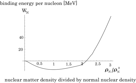
Figure 1: Nuclear matter saturation properties with $m_{N}(\rho_{N}^{0})=0.6m_{N}(\rho_{N}=0)$: Parameters are summarized in Table I. Then, the imcompressibility is $K=260$ [MeV].

4.2 Quark Matter

For quark matter, we set $G_{v}^{q}=0$ in Eq.(1) as was already mentioned in the preceeding section. As for the model parameters, the coupling constant $G_{s}^{q}$ and the three momentum cutoff $\Lambda_{q}$ are determined from the dynamical quark mass and the pion decay constant in the vacuum in Eq.(3.2). The parameters are summarized in Table II.

4.2.1 $G_{sv}^{q}=0$

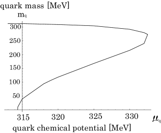
Figure 2: The solutions of the gap equations for quark mass are depicted as a function of the quark chemical potential $\mu_{q}$ with $G_{sv}^{q}=0$ for the original NJL model. The vertical axis represents the dynamical quark mass $m_{q}$ and the horizontal axis represents the quark chemical potential $\mu_{q}$.

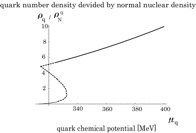
Figure 3: The quark number density versus quark chemical potential is depicted at $T=0$. The dashed curve is not realized physically.

First, we use the original NJL model Lagrangian density without the vector-scalar ($G_{sv}^{q}$) interactions, namely, we put $G_{sv}^{q}=0$.

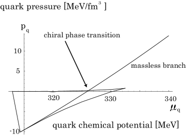
Figure 4: The pressure versus chemical potential is depicted at $T=0$. The chiral phase transition occurs at $\mu_{q}\approx 326$ MeV.

We solve the gap equation in Eq.(3) with $G_{sv}^{q}=0$ under a finite quark chemical potential $\mu_{q}$ at zero temperature. Then, the dynamical quark mass $m_{q}$ is obtained at finite quark chemical potential. In Fig.2, the dynamical quark mass is depicted as a function of the quark chemical potential. For $\mu_{q}=313$ MeV, the vacuum value for the dynamical quark mass is obtained. From Eq.(9) at zero temperature, we obtain the relation between the quark number density $\rho_{q}$ and the quark chemical potential $\mu_{q}$. In Fig.3, the quark number density is depicted as a function of the quark chemical potential. The vertical axis represents the quark number density divided by the normal nuclear density, namely, $\rho_{q}/\rho_{N}^{0}$. The dashed curves represent the unphysical region. Namely, the gap equation has multiple solutions in a certain region as is seen from Fig.2. Then, we must determine which solution is realized physically. For this purpose, the pressure is calculated from the thermodynamical potential density $\omega$ in Eq.(12) by the same subtraction method as the energy density per single nucleon in Eq.(23):

$$-p_{i}(T,\mu_{i})=(\langle\!\langle{\cal H}_{i}^{MF}\rangle\!\rangle(T,\mu_{i})-\langle\!\langle{\cal H}_{i}^{MF}\rangle\!\rangle(T=0,\mu_{i}=m_{i}(T=0)))$$

$$\qquad\qquad\qquad-\mu_{i}\langle\!\langle{\cal N}_{i}\rangle\!\rangle-\frac{1}{\beta}\langle\!\langle{\cal S}_{i}\rangle\!\rangle\ ,$$ (27)

where $i=q$ for the quark matter. The physical solution corresponds to the one which gives the largest pressure. In Fig.4, the pressure $p_{q}$ is depicted as a function of the quark chemical potential $\mu_{q}$. From $\mu_{q}=313$ MeV to about $326$ MeV, the low density solution is realized seen from Fig.3. However, above $\mu_{q}\approx 326$ MeV, the massless solution is physically realized. From Fig.4, it is seen that the chiral phase transition occurs at $\mu_{q}\approx 326$ MeV. In this case, in the region from $\rho_{q}\sim 0.28\rho_{N}^{0}$ to $\rho_{q}\sim 5.41\rho_{N}^{0}$ (from $\rho_{B}\sim 0.09\rho_{N}^{0}$ to $\rho_{B}\sim 1.80\rho_{N}^{0}$ where $\rho_{B}$ represents the baryon number density) as is seen in Fig.3, the first order chiral phase transition is realized and quark phases coexistence occurs. It seems that this density is rather small compared with the quark-hadron phase transition as is mentioned below.

4.2.2 $G_{sv}^{q}\Lambda_{q}^{8}=-68.4$

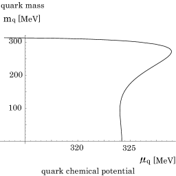
Figure 5: The solutions of the gap equations for quark mass are depicted as a function of the quark chemical potential $\mu_{q}$ at $T=0$ with $G_{sv}^{q}\Lambda_{q}^{8}=-68.4$.

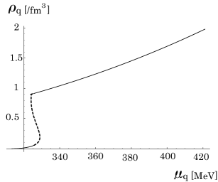
Figure 6: The quark number density $\rho_{q}$ versus quark chemical potential $\mu_{q}$ is depicted at $T=0$ with $G_{sv}^{q}\Lambda^{8}=-68.4$. The dashed curve is not realized physically.

In the original NJL model with $G_{sv}^{q}=0$, it seems that the chiral phase transition occurs at rather small density. One of possible reasons why the chiral phase transition occurs at rather small density may be that the strength of the attractive interaction between quark and antiquark is weak. So, the quark condensate is melt at rather small density. Thus, there exists one possibility that the attractive interaction becomes strong by introducing the scalar-vector attractive interaction $G_{sv}^{q}$ for the original quark NJL model.

However, there is no criterion to determine the value of $G_{sv}^{q}$ in this stage. Thus, as is the first attempt, we regard $G_{sv}^{q}$ as a free parameter. First, we give the value $G_{sv}^{q}\Lambda_{q}^{8}=-68.4$, in which $m_{q}(\rho_{q}/3=\rho_{N}^{0})=0.625m_{q}(\rho_{q}=0)$.

In Fig.5, the dynamical quark mass is depicted as a function of the quark chemical potential. For $\mu_{q}=313$ MeV, the vacuum value for the dynamical quark mass is also obtained. In Fig.6, the quark number density $\rho_{q}$ itself is depicted as a function of the quark chemical potential $\mu_{q}$. The dashed curves represent the unphysical region, as is similar to Fig.3. Namely, the gap equation has multiple solutions in a certain region. Then, we must determine which solution is realized physically by comparing with each pressure. In Fig.7, the pressure for each branch is depicted as a function of the quark chemical potential $\mu_{q}$.

From Fig.7, it is seen that the chiral phase transition occurs at $\mu_{q}\approx 326$ MeV. In this case, in the region from $\rho_{q}\sim 0.38\rho_{0}$ to $\rho_{q}\sim 5.41\rho_{0}$ (from $\rho_{B}\sim 0.12\rho_{0}$ to $\rho_{B}\sim 1.80\rho_{0}$), the chiral phase transition is realized and quark phases coexistence occurs.

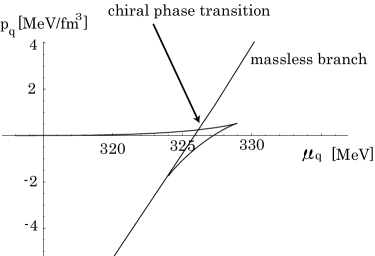
Figure 7: The pressure versus quark chemical potential is depicted and the chiral phase transition is shown at $T=0$ with $G_{sv}^{q}\Lambda^{8}=-68.4$.

4.2.3 $G_{sv}^{q}\Lambda_{q}^{8}=-225$

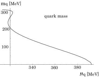
Figure 8: The solutions of the gap equations for quark mass are depicted as a function of the quark chemical potential $\mu_{q}$ at $T=0$ with $G_{sv}^{q}\Lambda^{8}=-225$.

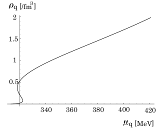
Figure 9: The quark number density $\rho_{q}$ versus quark chemical potential $\mu_{q}$ is depicted at $T=0$ with $G_{sv}^{q}\Lambda^{8}=-225$.

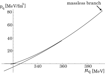
Figure 10: The pressure versus quark chemical potential is depicted and the chiral phase transition is shown at $T=0$ with $G_{sv}^{q}\Lambda^{8}=-225$.

Finally, we give the value $G_{sv}^{q}\Lambda_{q}^{8}=-225$ which leads to the dynamical quark mass at normal nuclear density as $m_{q}(\rho_{q}/3=\rho_{N}^{0})=0.681m_{q}(0)$.

In Fig.8, the dynamical quark mass is depicted as a function of the quark chemical potential. In Fig.9, the quark number density $\rho_{q}$ is depicted as a function of the quark chemical potential $\mu_{q}$. In Fig.10, the pressure of each branch is depicted as a function of the quark chemical potential. From Fig.10, it is seen that the phase with massless quark is realized in the region of $\mu_{q}>392.5$ MeV. In this case, at $\rho_{q}\sim 9.43\rho_{N}^{0}$ ($\rho_{B}\sim 3.14\rho_{N}^{0}$), the chiral phase transition may be realized.

5 Quark-hadron phase transition

The main purpose of this paper is to investigate the quark-hadron phase transition in the extended NJL model developed in this paper. In this section, we investigate the realized phase by comparing the pressures of the nuclear and quark matters at zero temperature and the finite baryon chemical potential. It is shown that the first order quark-hadron phase transition is realized at zero temperature and the finite baryon chemical potential. In order to investigate the phase transition, the condition of the chemical equilibrium is demanded for the chemical potential $\mu_{N}$ and $\mu_{q}$. Here, the chemical potential per one baryon at the same baryon density should be considered for the chemical equilibrium as follows:

$$\mu_{N}(T)=3\mu_{q}(T)\ .$$ (28)

Also, the same pressures between the nuclear matter $p_{N}$ and the quark matters $p_{q}$ are necessary as

$$p_{N}(T,\mu_{N})=p_{q}(T,3\mu_{q})\ .$$ (29)

The pressure has already been defined in Eq.(4.2.1).

The crossing point of each pressure for nuclear matter and the quark matter presents the coexistence point of the nuclear and the quark phases and the phase with larger value of the pressure is realized except for the crossing point.

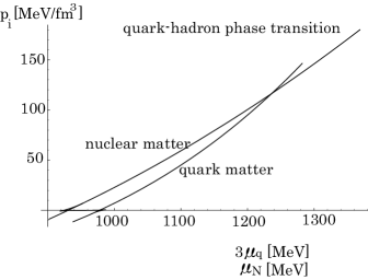
Figure 11: The quark-hadron phase transition is shown at $T=0$ with $G_{sv}^{q}\Lambda^{8}=-68.4$.

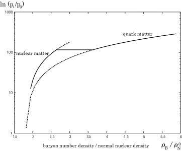
Figure 12: The quark-hadron phase transition is shown at $T=0$ with $G_{sv}^{q}\Lambda^{8}=-68.4$. The vertical axis and the horizontal axis represent the pressure $\ln(p_{i}/p_{0})$ and the baryon number density divided by the normal nuclear density $\rho_{B}/\rho_{N}^{0}$, respectively. Here, we use $p_{0}=1.0$ MeV/fm³.

In Fig.11, the pressures for the nuclear matter and the quark matter are depicted as functions of the nuclear chemical potential $\mu_{N}$ and the quark chemical potential multiplied by 3, $3\mu_{q}$, respectively, in the case $G_{sv}^{q}\Lambda_{q}^{8}=-68.4$. In this figure, it is shown that the quark-hadron phase transition occurs at a critical chemical potential value $\mu_{c}$ which is about $\mu_{c}(=\mu_{N}=3\mu_{q})\approx 1236$ MeV. From this figure, the nuclear or hadron phase is realized in the small chemical potential region $\mu_{N}<\mu_{c}$. However, in the large chemical potential region $3\mu_{q}>\mu_{c}$, the quark phase is realized. In terms of the baryon number density $\rho_{B}$ by using the relation of the density and chemical potential shown in Fig.6, from $\rho_{q}\sim 10.9\rho_{0}\ (\rho_{B}=\rho_{q}/3\sim 3.63\rho_{0})$ to $\rho_{N}(=\rho_{B})\sim 2.65\rho_{0}$, the nuclear and quark phases coexist and the first order quark-hadron phase transition is realized. This situation is depicted in Fig.12.

For the other parameter values for $G_{sv}^{q}$, the same figure is obtained. The reason is as follows: For these model parameters used in this paper, that is, $G_{sv}^{q}\Lambda_{q}^{8}=0$, $-68.4$ and $-225$, the quark-hadron phase transition point is in the chiral symmetric phase, that is, $m_{q}=0$ and $\langle{\overline{\psi}}_{q}\psi_{q}\rangle=0$. Namely, the quark-hadron phase transition from hadron phase to quark phase occurs after the chiral phase transition from chiral broken phase to chiral symmetric phase in these model parameters. This behavior for the phase transitions is also seen in Ref.12. Then, the pressure of quark matter $p_{q}$ in Eq.(4.2.1) with $T=0$ does not depend on $G_{sv}^{q}$ because $\langle{\cal H}_{q}^{MF}\rangle$ in Eq.(13) and $\mu_{q}^{r}$ in Eq.(6) does not depend on $G_{sv}^{q}$ due to $\langle{\overline{\psi}}_{q}\psi_{q}\rangle=0$. Thus, the behavior seen in Fig.12 is not changed.

6 Summary and concluding remarks

In this paper, the quark-hadron phase transition at finite baryon chemical potential has been described in the extended NJL model, in which both the nucleon in the nuclear matter and the quark in the quark matter were treated as fundamental fermions with a number of color, $N_{c}$, being one for nucleon and being three for quark. In this paper, as the first attempt of the investigation for the quark-hadron phase transition in the extended NJL model, we only dealt with the symmetric nuclear matter and the quark matter without quark-quark correlation leading to the pairing instability.

As for the symmetric nuclear matter, the saturation property has been well reproduced in this model. As for the quark matter, there is one free parameter, that is, the coupling strength of the scalar-vector eight-point interaction, $G_{sv}^{q}$. This model parameter controlls the chiral phase transition point and/or the strength of the partial restoration of the chiral symmetry in the nuclear medium. In this paper, we did not fix its value by using other physical quantity. This is a future problem.

We have calculated the pressures of nuclear matter and quark matter, respectively. Then, by comparing the pressure of nuclear matter with that of quark matter, the realized phase is determined. As a result, the first order quark-hadron phase transition is obtained at finite density and zero temperature. It should be noted here that, for the adopted parameter $G_{sv}^{q}$ used in this paper, the deconfinement phase transition occurs after the chiral symmetry restoration in the nuclear matter. Thus, the phase transitions in the quark phases may be hidden because they occur before quark deconfinement.

It is interesting to investigate the quark-hadron phase transition at finite temperature and baryon chemical potential because the phase diagram in the QCD world is not understood completely at present. It is also interesting to study the phase transition between the neutron matter and quark matter at finite density, which has important implications to the physics of neutron star. Of course, on the side of quark phase, the color superconducting phase should be taken into account. These are future problems in this model calculation.

References

• [1] B. D. Serot and J. D. Walecka, Advances in Nuclear Physics, Vol.16, eds. J. W. Negele and E. Vogt (Plenum, New York, 1986).
• [2] Y. Nambu and G. Jona-Lasinio, Phys. Rev. 122 (1961), 345; ibid. 124 (1961), 246.
• [3] S. P. Klevansky, Rev. Mod. Phys. 64 (1992), 649.
T. Hatsuda and T. Kunihiro, Phys. Rep. 247 (1994), 221.
• [4] M. Buballa, Phys. Rep. 407 (2005), 205.
• [5] W. Bentz and A. W. Thomas, Nucl. Phys. A 693, 138 (2001).
• [6] V. Koch, T. S. Biro, J. Kunz and U. Mosel, Phys. Lett. B185 (1987), 1.
• [7] S. A. Moszkowski, C. Providência, J. da Providência and J. M. Moreira, nucl-th/0204047.
• [8] C. Providência, J. da Providência and S. A. Moszkowski, in “Proceedings of the 11the International Conferences on Recent Progress in Many-Body Theories”, R. F. Bishop, K. A. Gernoth, N. R. Walet and Y. Xian (Eds.) (World Scientific, Singapole, 2002) p.242.
C. Providência, J. M. Moreira, J. da Providência and S. A. Moszkowski, in “Hadron Physics : Effective Field Theories of Low Energy QCD”, A. Blin, B. Hiller, M. C. Ruivo and E. van Beveren (Eds.) AIP Conference Proceedings, Vol.660 (New York, 2003) p.231.
• [9] M. G. Alford, A. Schmitt, K. Rajagopal and T. Schafer, Rev. Mod. Phys. 80 (2008), 1445.
• [10] D. P. Menezes and C. Providência, Phys. Rev. C68, 035804 (2003).
• [11] T. Matsubara, Prog. Theor. Phys. 14 (1955), 351.
• [12] H. Bohr, C. Providência and J. da Providência, Phys. Rev. C 71 (2005), 055203.