On the Border Length Minimization Problem (BLMP) on a Square Array

Abstract

Protein/Peptide microarrays are rapidly gaining momentum in the diagnosis of cancer. High-density and high-throughput peptide arrays are being extensively used to detect tumor biomarkers, examine kinase activity, identify antibodies having low serum titers and locate antibody signatures. Improving the yield of microarray fabrication involves solving a hard combinatorial optimization problem called the Border Length Minimization Problem $(BLMP)$. An important question that remained open for the past seven years is if the BLMP is tractable or not. We settle this open problem by proving that the BLMP is $\cal NP$-hard. We also present a hierarchical refinement algorithm which can refine any heuristic solution for the BLMP problem. We also prove that the TSP+1-threading heuristic is an $O(N)$-approximation.

The hierarchical refinement solver is available as an open-source code at http://launchpad.net/blm-solve.

Complexity of proof procedures] Graph Algorithms] Reducibility and completeness]

1 Introduction

Cancer diagnosis research has taken a new direction recently by adopting peptide microarrays for reliable detection of tumor biomarkers (Chatterjee, et al., [1]), (Melle, et al., [7]), (Welsh, et al., [8]). These high-throughput arrays also find application in examining kinase activity, identifying antibody signatures against tumor antigens, etc. High-density peptide arrays are currently fabricated using technologies such as photolithography or in-situ synthesis based on micromirror arrays. The manufacturers of these arrays are facing serious fabrication challenges due to unintended illumination effects such as diffraction and scattering of light. These illumination effects can be reduced dramatically by selecting a right placement of the peptide probes before fabrication. Finding this placement can be formulated as a combinatorial optimization problem, known as the Border Length Minimization Problem (BLMP). Hannenhalli, et al. first introduced BLMP in 2002 [4]. Although the BLMP was formulated in the context of DNA microarrays, peptide arrays share a similar fabrication technology.

The BLMP can be stated as follows. Given $N^{2}$ strings of the same length, how do we place them in a grid of size $N\times N$ such that the Hamming distance summed over all the pairs of neighbors in the grid is minimized? The BLMP has received a lot of attention from many researchers. The earliest algorithm suggested by Hannenhalli, et al. reduces BLMP to TSP (Traveling Salesman Problem) by computing a tour of the strings and then threading the tour on the grid [4]. Kahng, et al. have proposed several other heuristic algorithms which are considered the best performing algorithms in practice [5]. De Carvalho, et al. introduced a quadratic program formulation of the BLMP but unfortunately the quadratic program is an intractable problem [3]. Later, Kundeti and Rajasekaran formulated the problem as an integer linear program which performs better than the quadratic program in practice [6].

Despite many studies on the BLMP, the question of whether BLMP is tractable or not remained open for the past 7 years. In this paper, we show that the BLMP is $\cal NP$-hard. We also consider a generalization of the BLMP called the Hamming Graph Placement Minimization Problem (HGPMP). We show that some special cases of the HGPMP are also $\cal NP$-hard. On the algorithmic side, we show that a simple version of the algorithm suggested by Hannenhalli, et al. is an $O(N)$-approximation. On the practical side, we propose a refinement algorithm which takes any solution and tries to improve it. An experimental study of this refinement algorithm is also included.

Our paper is organized as follows. Section 2 formally defines the BLMP and HGPMP. Section 3 provides the $\cal NP$-hardness proof of the BLMP and some special cases of the HGPMP. Section 4 gives the $O(N)$-approximation algorithm and the refinement algorithm for the BLMP. Section 5 provides an experimental evaluation of the refinement algorithm. Finally, Section 6 concludes our paper and discusses some open problems.

2 Problem definition

Let $S$ be a set of strings of the same length with $S=\{s_{1},\dots,s_{n}\}$ and let $G=(V,E)$ be a graph with $|V|=n$. A placement of $S$ on $G$ is a bijective map $f:S\rightarrow V$. Let $f^{-1}(u)$ be the string that is mapped to vertex $u$ by the placement $f$. We denote the Hamming distance between two strings $s_{i}$ and $s_{j}$ as $\delta(s_{i},s_{j})$. The cost of placement $f$ is $Cost(f)=\sum_{e=(u,v)\in E}\delta(f^{-1}(u),f^{-1}(v))$. The Hamming Graph Placement Minimization Problem (HGPMP) is defined as follows. Given $S$ and $G$, find a placement of $S$ on $G$ of minimum cost. We denote the optimal cost as $OPT(S,G)$, or simply as $OPT$ if it is clear what $S$ and $G$ are.

Obviously, if $G$ is a ring graph, then HGPMP is the same as the well-known Hamming Traveling Salesman Problem (HTSP). If $G$ is a grid graph of size $N\times N$ (where $N^{2}=n$), then HGPMP becomes the Border Length Minimization Problem (BLMP), which is the main study of our paper.

3 $\cal NP$-hardness of the BLMP
and HGPMP

Theorem 1

The BLMP is $\cal NP$-hard.

We will show that the Hamming traveling salesperson problem (HTSP) for strings (with the Hamming distance metric) polynomially reduces to the BLMP. The HTSP is already defined in Section 2.

The idea of the proof is that given $4N$ strings for the HTSP we construct $(N+1)^{2}$ strings for the BLMP such that from an optimal solution to this BLMP, we can easily obtain an optimal solution for the HTSP. So we need to consider the variant of the HTSP in which the number of strings is divisible by $4$. The proof will be presented in stages. The next three subsections present some preliminaries needed for the proof of the theorem. Followed by these subsections, the proof is presented.

3.1 $4N$-strings traveling salesperson problem

Define an instance of the HTSP as a $4N$-strings HTSP if the number of strings in the input is $4N$ (for some integer $N$). In this section we show that the $4N$-strings HTSP is $\cal NP$-hard.

Theorem 2

$4N$-strings HTSP is $\cal NP$-hard.

Proof: We will show that the HTSP polynomially reduces to the $4N$-strings HTSP. Let $S=\{s_{1},s_{2},\ldots,s_{n}\}$ be the input for any instance of the HTSP. Let $\ell$ be the length of each input string. Append a string of $2n\ell$ $\overline{0}$’s to the left of each $s_{i}$ to get $s_{i}^{\prime}$ (for $1\leq i\leq(n-1))$. For example, if $n=4,\ell=3$ and $s_{1}=\overline{101}$, then $s_{1}^{\prime}$ will be $\overline{000000000000000000000000101}$. We append $2n\ell$ $\overline{1}$’s to the left of $s_{n}$ to get $s_{n}^{\prime}$. We will generate an instance $S^{\prime}$ of the $4N$-strings HTSP that has as input $4N$ strings, where $N=\lceil\frac{n}{4}\rceil$. $S^{\prime}$ will have $s_{1}^{\prime},s_{2}^{\prime},\ldots,s_{n-1}^{\prime}$ and $1,2,3$ or $4$ copies of $s_{n}^{\prime}$ depending on whether $n=4N,4N-1,4N-2$, or $4N-3$, respectively.

It is easy to see that in an optimal tour for the above $4N$-strings HTSP instance, all the copies of $s_{n}^{\prime}$ will be successive and that an optimal solution for $S$ can be obtained readily from an optimal solution for $S^{\prime}$. $\Box$

3.2 A special instance of the BLMP

Consider the following $(N+1)^{2}$ strings as an input for the BLMP:$t_{1},t_{2},\dots,t_{4N},t,t,\dots,t$. Here there are $N^{2}-2N+1$ copies of $t$. There is a positive integer $k$ such that $\delta(t_{i},t)=k$ for any $1\leq i\leq 4N$ and $2k\geq\delta(t_{i},t_{j})>\frac{7}{4}k$ for any $1\leq i\neq j\leq 4N$.

Lemma 1

In any optimal solution to the above BLMP instance, $t_{1},t_{2},\ldots,t_{4N}$ will lie on the boundary of the $(N+1)\times(N+1)$ grid (see Figure 1).

Proof: This can be proven by contradiction. Let $T$ be the collection of the strings $t_{1},t_{2},\ldots,t_{4N}$. Let $q$ be one of the strings from $T$ that has a degree of 4 in an optimal placement. Let $r$ be one of the strings equal to $t$ that lies in the boundary. Next we show that we can get a better solution by exchanging $q$ and $r$.

Let $u$ be the number of neighbors of $q$ from $T$. Let $v$ be the number of neighbors of $r$ from $T$. Note that $0\leq u\leq 4$ and $0\leq v\leq 3$. In the current solution, the total cost incurred by $q$ and $r$ is at least $\frac{7}{4}ku+k(4-u)+kv=\frac{3}{4}ku+kv+4k$. If we exchange $q$ and $r$, the new total cost incurred by $q$ and $r$ is strictly less than $ku+2kv+k(3-v)=ku+kv+3k$. The old cost minus the new cost is strictly greater than $k-\frac{1}{4}ku\geq 0$.

We thus conclude that all the strings of $T$ lie on the boundary of the grid in any optimal solution. $\Box$

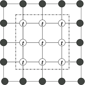
Figure 1: An illustration for Lemma 1 with $N=4$. Each $t_{i}$ lies on a dark vertex in the grid.

3.3 A special set of strings and some operations on strings

We denote the (ordered) concatenation of two strings $x$ and $y$ as $x+y$. If $x$ and $x^{\prime}$ (respectively $y$ and $y^{\prime}$) have the same length then, clearly, $\delta(x+y,x^{\prime}+y^{\prime})=\delta(x,x^{\prime})+\delta(y,y^{\prime})$.

Given a string $x=\overline{x_{1}x_{2}\dots x_{l}}$ and an integer $h$, let $REP_{h}(x)$ be the string $\overline{x_{1}x_{1}\dots x_{1}x_{2}x_{2}\dots x_{2}\dots x_{l}x_{l}\dots x_{l}}$, where each $x_{i}$ appears $h$ times ($REP$ stands for “replicate”). It is not hard to see that if $x$ and $y$ have the same length, then $\delta(REP_{h}(x),REP_{h}(y))=h\delta(x,y)$.

Given an integer $n$, we can construct a set of $n$ strings of length $n$ each, $A_{n}=\{a_{1},a_{2},\dots,a_{n}\}$, such that $\delta(a_{i},a_{j})=2$ for any $1\leq i\neq j\leq n$. One way to construct $A_{n}$ is to let $a_{i}=\overline{00\dots 0100\dots 0}$, where there are $(i-1)$ $\overline{0}$’s before $\overline{1}$. It is easy to check that $\delta(a_{i},a_{j})=2$ for any $1\leq i\neq j\leq n$.

3.4 Proof of the main theorem

Now we are ready to present the proof of Theorem 1. Let $S=\{s_{1},s_{2},\ldots,s_{4N}\}$ be the input for any instance of the $4N$-strings HTSP. Each $s_{i}$ has the length $l$. We will generate $(N+1)^{2}$ strings such that an optimal solution for the BLMP on these $(N+1)^{2}$ strings will yield an optimal solution for the $4N$-strings HTSP on $S$.

The input for the BLMP instance that we generate will be$T=\{t_{1},t_{2},\ldots,t_{4N},t,t,\ldots,t\}$ where $t$ occurs $N^{2}-2N+1$ times. We set $t_{i}=REP_{h}(a_{i})+REP_{2}(s_{i})$, where $a_{i}$ is the $i$-th string in the set $A_{4N}$ defined in subsection 3.3. We will choose $h$ later. Also, we set $t=REP_{4Nh}(\overline{0})+\overline{0101\dots 01}$, where the string $\overline{01}$ is repeated $l$ times. We can easily check that:

$$\delta(t_{i},t) = h+l\,\,\mbox{ for any }1\leq i\leq 4N$$ (1)

$$\delta(t_{i},t_{j}) = 2h+2\delta(s_{i},s_{j})\leq 2h+2l$$

$$\mbox{ for any }1\leq i\neq j\leq 4N$$

We choose $h$ so that $T$ satisfies the condition in Lemma 1. Particularly, choose $h=8l$. Now we will show that $OPT_{BLMP}(T)=4(N-1)(h+l)+8Nh+2OPT_{HTSP}(S)$, which in turn means that an optimal solution for the BLMP on $T$ will yield an optimal solution for the $4N$-strings HTSP on $S$.

Let $A=s_{i_{1}},s_{i_{2}},\dots,s_{i_{4N}}$ be an optimal tour for the $4N$-string HTSP on $S$. We construct a solution $A^{\prime}$ for the BLMP on $T$ by placing $t_{i}$’s on the border of the grid in the order $t_{i_{1}},t_{i_{2}},\dots,t_{i_{4N}}$ and placing the copies of $t$ on the center of the grid. By the equalities (1) and (3.4), the cost of $A^{\prime}$ is $Cost(A^{\prime})=4(N-1)(h+l)+8Nh+2Cost(A)$. Therefore, $OPT_{BLMP}(T)\leq 4(N-1)(h+l)+8Nh+2OPT_{HTSP}(S)$.

On the other hand, let $B$ be an optimal solution for the BLMP on $T$. By Lemma 1, $t_{i}$’s lie on the border of the grid and the copies of $t$ lie on the center of the grid. Assume that $t_{i}$’s lie in the order $t_{i_{1}},t_{i_{2}},\dots,t_{i_{4N}}$. We can construct a tour $B^{\prime}$ for the $4N$-strings HTSP on $S$ in the order $s_{i_{1}},s_{i_{2}},\dots,s_{i_{4N}}$. By the equalities (1) and (3.4), $Cost(B)=4(N-1)(h+l)+8Nh+2Cost(B^{\prime})$. Hence, $OPT_{BLMP}(T)\geq 4(N-1)(h+l)+8Nh+2OPT_{HTSP}(S)$.

This completes the proof of Theorem 1. $\Box$

3.5 $\cal NP$-hardness of the HGPMP for other special cases

We can generalize the result in Theorem 1 for other special cases of the HGPMP. We say graph $G$ is “bordered-ring" if $G$ is undirected and $G$ has a ring of size $\Omega(n^{\alpha})$ for some constant $\alpha>0$ such that every vertex in the ring has degree no greater than $d$ and every vertex outside the ring has degree greater than $d$ for some $d\geq 3$. For grid graphs, $\alpha=\frac{1}{2}$ and $d=3$. Some variants of grid graphs like Manhattan grids are bordered-ring as well.

Theorem 3

The HGPMP is $\cal NP$-hard even if $G$ is bordered-ring.

Proof: By a similar reduction to that of the BLMP above, the theorem follows. $\Box$

3.6 An alternate $\cal NP$-hardness proof
for the BLMP

In this section, we give an alternate $\cal NP$-hardness proof for the BLMP by showing that another variant of the HTSP called $k$-Segments HTSP polynomially reduces to the BLMP. We believe that the techniques introduced in both of our proofs will find independent applications.

3.6.1 $k$-Segments traveling salesperson problem

We define the $k$-segments HTSP and show that it is NP-hard. Consider an input of $n$ strings: $s_{1},s_{2},\ldots,s_{n}$. The problem of $k$-segments HTSP is to partition the $n$ strings into $k$ parts such that the sum of the optimal tour costs for the individual parts is minimum.

Theorem 4

The $k$-segments HTSP for strings is $\cal NP$-hard.

Proof: We will prove this for $k=4$ (since this is the instance that will be useful for us to prove the main result) and the theorem will then be obvious.

We will show that the HTSP polynomially reduces to the $4$-segments HTSP. Let $S=\{s_{1},s_{2},\ldots,s_{n}\}$ be the input to any instance of the HTSP. We will generate an instance of the $4$-segments HTSP that has as input $(n+3)$ strings. Let $l$ be the length of each string in $S$. Note that the optimal cost for the HTSP with input $S$ is $\leq nl$.

Consider the 4 strings: $\overline{1110},~{}\overline{1101},~{}\overline{1011},~{}\overline{0111}$. The distance between any two of them is $2$. Now replace each $\overline{1}$ in each of these $4$ strings with a string of $nl$ $\overline{1}$’s. Also, replace each $\overline{0}$ in each of these strings with a string of $nl$ $\overline{0}$’s. Call these new strings $t_{1},t_{2},t_{3},t_{4}$. The distance between any two of these strings is $2nl$.

The input strings for the $4$-segments HTSP are $q_{1},q_{2},\ldots,q_{n+3}$ and are constructed as follows: $q_{i}$ is nothing but $s_{i}$ with $t_{1}$ appended to the left, for $1\leq i\leq n$. $q_{n+1}$ is a string of length $4nl+l$ whose $l$ LSBs are $\overline{0}$’s and whose $4nl$ MSBs equal $t_{2}$. $q_{n+2}$ is a string of length $4nl+l$ whose $l$ LSBs are $\overline{0}$ and whose $4nl$ MSBs equal $t_{3}$. Also, $q_{n+3}$ has all $\overline{0}$’s in its $l$ LSBs and its $4nl$ MSBs equal $t_{4}$.

Clearly, in an optimal solution for the $4$-segments HTSP instance, the four parts have to be $\{q_{1},q_{2},\ldots,q_{n}\},~{}\{q_{n+1}\},~{}\{q_{n+2}\}$, and $\{q_{n+3}\}$. As a result, we can get an optimal solution for the HTSP instance given an optimal solution for the $4$-segments HTSP instance. $\Box$

3.6.2 A special instance of the BLMP

Consider the following $n^{2}$ strings as an input for the BLMP:$t_{1},t_{2},\ldots,t_{n},t,t,\ldots,t$. Here there are $n^{2}-n$ copies of $t$. Also, $\delta(t_{i},t_{j})=16$ for any $i$ and $j$ less than or equal to $n$. $\delta(t_{i},t)=9$ for any $i\leq n$.

Lemma 2

In an optimal solution to the above BLMP instance, $t_{1},t_{2},\ldots,t_{n}$ lie on the boundary of the $n\times n$ grid and moreover these strings are found in four segments of successive nodes.

Proof: Let $T$ be the collection of strings $t_{1},t_{2},\dots,t_{n}$. By Lemma 1, we conclude that all the strings of $T$ lie on the boundary of the grid in an optimal solution.

Let $S_{1}$ and $S_{2}$ be two segments such that $S_{1}$ and $S_{2}$ consist of strings from $T$, strings in $S_{1}$ are in successive nodes, strings in $S_{2}$ are in successive nodes, and these two segments are not successive. Consider the case when none of these strings is in a corner of the grid. Let $S_{1}=\{a_{1},a_{2},\ldots,a_{n_{1}}\}$ and $S_{2}=\{b_{1},b_{2},\ldots,b_{n_{2}}\}$. Let $C(S_{1})=\sum_{i=1}^{n_{1}-1}\delta(a_{i},a_{i+1})$ and $C(S_{2})=\sum_{i=1}^{n_{2}-1}\delta(b_{i},b_{i+1})$. The total cost for these two segments is $C(S_{1})+C(S_{2})+9(n_{1}+n_{2})+36$. If we join these two segments into one, the new cost will be $C(S_{1})+C(S_{2})+9(n_{1}+n_{2})+34$.

Thus it follows that all the strings of $T$ will be on the boundary and they will be found in successive nodes in any optimal solution. Also it helps to utilize the corners of the grid since each use of a corner will reduce the total cost by 9. Therefore in an optimal solution there will be four segments such that all the segments are in the boundary of the grid, each segment has strings from $T$ in successive nodes, and one string of each segment occupies a corner of the grid. In other words, an optimal solution for the BLMP instance contains an optimal solution for the 4-segments TSP corresponding to $T$. The optimal cost for this BLMP instance is $25n-28$. $\Box$

3.6.3 Construction of strings for the above BLMP instance

We can construct $n^{2}$ strings that have the same properties as the ones in the above BLMP instance.

To begin with, we construct $(n+1)$ binary strings of length $n$ each. The string $t_{i}$ has all $\overline{1}$’s except in position $i$, for $1\leq i\leq n$. The position of the LSB of any string is assumed to be $\overline{1}$. String $t_{n+1}$ has all $\overline{1}$’s. Clearly, $\delta(t_{i},t_{j})=2$ for any $i$ and $j$ less than or equal to $n$. Also, $\delta(t_{i},t_{n+1})=1$ for any $1\leq i\leq n$.

Now, in each $t_{i}$ (for $1\leq i\leq(n+1)$) replace every $\overline{1}$ with a string of eight $\overline{1}$’s and replace each $\overline{0}$ with a string of eight $\overline{1}$’s. After this change, $\delta(t_{i},t_{j})=16$ for any $1\leq i,j\leq n$ and $\delta(t_{i},t_{n+1})=8$ for any $1\leq i\leq n$.

Finally, append a $\overline{0}$ to the left of each $t_{i}$ (for $1\leq i\leq n$) as the MSB. Also, append a $\overline{1}$ to the left of $t_{n+1}$. In this case, $\delta(t_{i},t_{j})=16$ for any $1\leq i,j\leq n$ and $\delta(t_{i},t_{n+1})=9$ for any $1\leq i\leq n$.

3.6.4 The alternate proof of the main theorem

Let $S=\{s_{1},s_{2},\ldots,s_{n}\}$ be the input for any instance of the HTSP. We will generate $n^{2}$ strings such that an optimal solution for the BLMP on these $n^{2}$ strings will yield an optimal solution for the $4$-segments HTSP on $S$.

We will use as the basis the $(n+1)$ strings generated in the above section. Recall that these strings $t_{1},t_{2},\ldots,t_{n+1}$ are of length $(8n+1)$ each. Also, $\delta(t_{i},t_{j})=16$ for any $1\leq i,j\leq n$ and $\delta(t_{i},t_{n+1})=9$ for any $1\leq i\leq n$.

Replace each $\overline{0}$ in each of the above strings with $nl$ $\overline{0}$’s and replace each $\overline{1}$ in each of these strings with $nl$ $\overline{1}$’s. Now, $\delta(t_{i},t_{j})=16nl$ for any $1\leq i,j\leq n$ and $\delta(t_{i},t_{n+1})=9nl$ for any $1\leq i\leq n$. Each of these strings is of length $(8n+1)nl$.

Replace each $\overline{0}$ in each $s_{i}$ with two $\overline{0}$’s (for $1\leq i\leq n$) and replace each $\overline{1}$ in each $s_{i}$ with two $\overline{1}$’s and let $s^{\prime}_{i}$ be the resultant string. Note that an optimal solution for the $4$-segments HTSP on the revised $S$ will also be an optimal solution for the $4$-segments HTSP on the old $S$. If $l$ is the length of each string in the old $S$, then $2l$ will be the length of each revised input string.

The input for the BLMP instance that we generate will be $q_{1},q_{2},\ldots,q_{n},t,t,\ldots,t$ where $t$ occurs $n^{2}-n$ times. Each of these strings will be of length $(8n+1)nl+2l$. The string $q_{i}$ will have $s^{\prime}_{i}$ in its $2l$ LSBs and it will have $t_{i}$ in its $(8n+1)nl$ MSBs, for $1\leq i\leq n$. The string $t$ will have $t_{n+1}$ in its $(8n+1)nl$ MSBs. Its $2l$ LSBs will be $\overline{0101\ldots 01}$, i.e., the string $\overline{01}$ is repeated $l$ times. Note that $\delta(q_{i},q_{j})=16nl+\delta(s^{\prime}_{i},s^{\prime}_{j})$ for any $1\leq i,j\leq n$. Also, $\delta(q_{i},t)=9nl+l$ for any $1\leq i\leq n$.

Note that strings of this BLMP instance are comparable to the strings we had for Lemma 2. This is because the interstring distances are very nearly in the same ratios for the two cases. As a result, using a proof similar to that of Lemma 2, we can show that the strings $t_{1},t_{2},\ldots,t_{n}$ will all lie in the boundary of the grid in an optimal solution to the above BLMP. Let $T=\{t_{1},t_{2},\ldots,t_{n}\}$. Also, the strings of $T$ will be found in four segments such that one string of each segment occupies one of the corner nodes of the grid. Let $S_{1},S_{2},S_{3},$ and $S_{4}$ stand for the strings in these four segments, respectively. Let $C_{1},C_{2},C_{3}$, and $C_{4}$ be the optimal tour costs for $S_{1},S_{2},S_{3}$, and $S_{4}$, respectively.

Let $|S_{i}|=n_{i}$ for $1\leq i\leq 4$. The total cost (i.e., the border length) for the above BLMP solution can be computed as follows. Consider $S_{1}$ alone. The cost due to this segment is $C_{1}+2(9nl+l)+(n_{1}-1)(9nl+l)$. The cost $2(9nl+l)$ is due to the two end points of the segment $S_{1}$. The cost $(n_{1}-1)(9nl+l)$ is due to the fact that each string of $S_{1}$ (except for the one in a corner of the grid) is a neighbor of a $t$. Upon simplification, the cost for $S_{1}$ is $C_{1}+(n_{1}+1)(9nl+l)$. Summing over all the four segments, the total cost for the BLMP solution is $C_{1}+C_{2}+C_{3}+C_{4}+(n+4)(9nl+l)$. The minimum value of this is obtained when $S_{1},S_{2},S_{3}$, and $S_{4}$ form a solution to the $4$-segments HTSP on $T$.

Clearly, an optimal solution for the $4$-segments HTSP on $T$ will also yield an optimal solution for the $4$-segments HTSP on $S$. This can be seen as follows. Consider the strings in $S_{i}$ and let $Q_{i}=a^{i}_{1},a^{i}_{2},\ldots,a^{i}_{n_{i}}$ be the corresponding input strings (of $S$), for $1\leq i\leq 4$. Note that $C_{i}$ is nothing but $(n_{i}-1)(16nl)$ plus twice the optimal tour cost for $Q_{i}$, for $1\leq i\leq 4$. Thus, $C_{1}+C_{2}+C_{3}+C_{4}$ is equal to $(n-4)16nl+2(C^{\prime}_{1}+C^{\prime}_{2}+C^{\prime}_{3}+C^{\prime}_{4})$ where $C^{\prime}_{i}$ is the optimal tour cost for $Q_{i}$, for $1\leq i\leq 4$.

This completes the proof of Theorem 1. $\Box$

4 Algorithms for the BLMP

4.1 An $O(N)$-approximation algorithm

In this section, we will show that a simple version of the algorithm suggested by Hannenhalli, et al. is actually an $O(N)$-approximation algorithm. This algorithm can be described as follows. Assume that the input is the set of strings $S=\{s_{1},s_{2},\dots,s_{N^{2}}\}$. The algorithm first computes a tour $T$ on strings in $S$. Then it threads the tour $T$ into the grid in row-major order (see Figure 2). The first step can be done by calling the $\frac{3}{2}$-approximation algorithm for the HTSP suggested by [2].

Figure 2: The thick dark line corresponds to an optimal tour on the input strings

Lemma 3

$OPT_{HTSP}(S)\leq 2OPT_{BLMP}(S)$.

Proof: Let $A$ be an optimal solution for the BLMP on $S$. Consider the path $P^{\prime}$ drawn as the thick dark line in Figure 2. Obviously, $Cost(P^{\prime})\leq Cost(A)=OPT_{BLMP}(S)$. Let $s_{i_{1}}$ and $s_{i_{N^{2}}}$ be the two endpoints of $P^{\prime}$. Since the Hamming distance satisfies the triangular inequality, $\delta(s_{i_{1}},s_{i_{N^{2}}})\leq Cost(P^{\prime})$. Consider the tour that starts at $s_{i_{1}}$, traverses along the path $P^{\prime}$ to $s_{i_{N^{2}}}$ and comes back to $s_{i_{1}}$. Obviously, the cost of the tour is $Cost(P^{\prime})+\delta(s_{i_{1}},s_{i_{N^{2}}})\leq 2Cost(P^{\prime})\leq 2Cost(A)$. Hence, $OPT_{HTSP}(S)\leq 2OPT_{BLMP}(S)$. $\Box$

Theorem 5

The above algorithm yields an $O(N)$-approximate solution.

Proof: First, we see that $Cost(T)\leq\frac{3}{2}OPT_{HTSP}(S)\leq 3OPT_{BLMP}(S)$. The first inequality is due to the $\frac{3}{2}$-approximation for the HTSP. The second inequality is due to Lemma 3. Now let us analyze the cost of the solution $F$ produced by the algorithm. Consider the path $P$ drawn as the thick dark line in Figure 2. Obviously, $Cost(P)\leq Cost(T)$. Also, the total cost of the $N$ rows in $F$ is no more than $Cost(P)$. By the triangle inequality, it is not hard to see that the cost of each column in $F$ is no more than $Cost(P)$. Therefore, $Cost(F)\leq(N+1)Cost(P)\leq(N+1)Cost(T)\leq 3(N+1)OPT_{BLMP}(S)=O(N)OPT_{BLMP}(S)$. $\Box$

4.2 A hierarchical refinement algorithm

Several heuristics such as the Epitaxial growth have been proposed to solve the BLMP problem earlier. However most of these heuristics do not improve the cost monotonically. Local search based algorithms are often employed to solve hard combinatorial problems. We now introduce a hierarchical refinement algorithm ($HRA$). This refinement technique can be applied to any heuristic placement to refine the cost and get a better placement. Let $N$ be the number of probes in the placement, $d$ a positive integer such that $d^{x}=N,x\geq 1$ is called the degree of refinement. The refinement algorithm starts with a given placement, then it divides the placement into $s^{0}_{1},s^{0}_{2}\ldots s^{0}_{N/d^{2}}$ sub-problems with $d^{2}$ probes per sub-problem. Each of these sub-problems is solved optimally – an optimal permutation among the probes is found. After this every $d^{2}$ sub-problems are combined into a new sub-problem $s^{1}_{i}=\displaystyle\cup_{j=1}^{d^{2}}s^{0}_{id^{2}+j},1\leq i\leq N/d^{3}$. To solve $s^{1}_{i}$ optimally we identify an optimal permutation among $s^{0}_{id^{2}+j}\in s^{1}_{i},1\leq j\leq d^{2}$. This process continues until we are left with no sub-problems to solve. See Figure 3.

We should remark that while solving a sub-problem optimally, we also consider the cost contributed from the neighboring sub-problems. This ensures the monotonic improvement in the placement cost. The refinement algorithm asymptotically runs in $\Theta(d^{2}!N)$ time. If $d=O(1)$, the refinement algorithm runs in linear time. For small values of $d$, the algorithm performs well in practice. $HRA$ is a deterministic refinement algorithm. We further extend this by introducing randomness. The Randomized Hierarchical Refinement Algorithm ($RHRA$) is similar to the $HRA$ algorithm. $RHRA$ randomly selects a sub-square within the given placement and applies the $HRA$ technique to the selected sub-square. Similar to local search algorithms, repeating $RHRA$ algorithm several times improves the placement cost monotonically. We study the performance of both these algorithms in section 5.

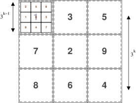
Figure 3: Illustration of the hierarchical refinement algorithm with degree of refinement $3$. This shows the possible optimal solutions (i.e. permutation among sub-problems) at the top-most and penultimate levels

4.3 Quad epitaxial algorithm

The epitaxial ($EPX$) placement suggested in [5] places a randomly selected probe at the center of the array, it continues placing the probes greedily around the locations adjacent to the placed probes to minimize the cost (i.e. the algorithm almost spends $O(N^{2})$ time to place each probe). The epitaxial algorithm gives good results for small arrays but for larger arrays the epitaxial algorithm is impractical and extremely slow. We propose the Quad Epitaxial ($QEPX$) algorithm as a simple extension to the epitaxial algorithm. $QEPX$ yields good performance and is very fast compared to the $EPX$ algorithm. The basic idea behind the $QEPX$ algorithm is to divide the array into four parts, apply $EPX$ algorithm for each of the four parts and finally find an optimal arrangement among the four parts. In section 5 we compare the $QEPX$ algorithm with $EPX$ algorithm.

5 Experimental study

5.1 Performance of the $QEPX$ algorithm

In this section we compare the performance of $QEPX$ algorithm introduced earlier. We use randomly generated probe arrays of size $32^{2}$,$64^{2}$,$128^{2}$ and $256^{2}$. In all of our experimental studies we compute a lower bound on the solution by picking the smallest $2N(N-1)$ edges from the complete Hamming distance graph. Column-$4$(INIT COST) in the table 1 indicates the placement cost obtained by placing the probes in the row major order as given by the input. Column-$5$($8$) indicates the final placement cost obtained by the epitaxial (quad) algorithm. As we can see from columns $7$ and $10$, the refinement obtained by the $QEPX$ algorithm is very close to the $EPX$ algorithm. On the other hand $QEPX$ runs $3.6X$ faster than the $EPX$ algorithm. As we can see from table 1, as the chip size increases $EPX$ algorithm becomes very slow. We ran both $EPX$ and $QEPX$ algorithms on a chip size of $243\times 243$ with a time limit of $60$ minutes. The $QEPX$ algorithm took around $12$ minutes to complete and improved the input placement cost by $36$%. On the other hand the $EPX$ algorithm did not complete the placement. From our experiments we conclude that the $QEPX$ can provide a good placement which we can use as an input for refinement/local search algorithms such as $RHRA$. In the next sub-section we provide our experimental study of $HRA$ and $RHRA$ algorithms on various placement heuristics.

TEST	PROBES	LOWER	INIT	EPX	TIME	REFINED	QEPX	TIME	REFINED
CASE		BOUND	COST		(sec)	PRECENT		(sec)	PRECENT
t-0	1024	23480	37192	27591	0.60	25.81%	28060	0.42	24.55%
t-1	1024	23427	37029	27472	0.62	25.81%	28151	0.43	23.98%
t-0	4096	86818	151116	106471	10.70	29.54%	107805	3.05	28.66%
t-1	4096	86897	151176	106430	10.37	29.60%	107634	3.23	28.80%
t-0	16384	322129	609085	410301	180.00	32.64%	411746	43.93	32.40%
t-1	16384	-	608928	409625	185.88	32.73%	410902	44.70	32.52%
t-0	65536	-	2447885	2447885	-	0.00%	1563369	765.79	36.13%
t-1	65536	-	2427143	2427143	-	0.00%	1562630	774.33	35.62%

Table 1: Comparison between epitaxial and quad epitaxial

PROBES	ALGO	LOWER	INIT	HRA	RHRA	REFINED	TIME
		BOUND	COST			PRECENT
729	RAND	17087	26401	23970	22631	14.280%	2.83(min)
729	SORT	17087	24082	22415	21649	10.103%	2.81(min)
729	SWM	17087	22267	22195	22069	0.889%	2.81(min)
729	REPTX	17087	21115	21107	21101	0.066%	2.81(min)
729	EPTX	17087	19733	19726	19726	0.035%	2.81(min)
6561	RAND	136820	243125	221090	209514	13.825%	17.55(min)
6561	SORT	136820	210326	198972	191915	8.754%	17.02(min)
6561	SWM	136820	204955	204525	203412	0.753%	17.20(min)
6561	REPTX	136820	185386	185362	185341	0.024%	17.16(min)
6561	EPTX	136820	168676	168623	168544	0.078%	17.15(min)
1024	RAND	23480	37192	35236	33046	11.148%	0.28(sec)
1024	SORT	23480	33784	32326	31026	8.164%	0.26(sec)
1024	SWM	23480	31424	31383	31323	0.321%	0.13(sec)
1024	QEPX	23480	28060	28035	28028	0.114%	0.47(sec)
1024	REPTX	23480	29574	29557	29546	0.095%	0.11(sec)
1024	EPTX	23480	27591	27567	27565	0.094%	0.11(sec)
4096	RAND	86818	151116	143246	134485	11.005%	6.93(sec)
4096	SORT	86818	131291	127033	121742	7.273%	4.46(sec)
4096	SWM	86818	127516	127357	127092	0.333%	1.27(sec)
4096	QEPX	86818	107805	107766	107702	0.096%	5.04(sec)
4096	REPTX	86818	116406	116395	116376	0.026%	1.02(sec)
4096	EPTX	86818	106471	106462	106448	0.022%	1.04(sec)

Table 2: Cost refinement for various placement heuristics by applying $HRA$ (hierarchical refinement algorithm) and $RHRA$ (randomized hierarchical refinement algorithm) with $350$ iterations

5.2 Performance of refinement algorithms

We have applied our $HRA$, $RHRA$ refining algorithms on the following placement heuristics.

• ($RAND$) Random placement: in this placement we just use the order in which the probes are provided to our algorithm.

• ($SORT$) Sort placement: in this placement the input probes are sorted lexicographically

• ($SWM$) Sliding Window Matching placement is obtained by running the $SWM$ [5] algorithm with parameters $(6,3)$.

• ($REPX$) Row epitaxial placement is obtained by running the row-epitaxial algorithm with $3$ look-ahead rows.

• ($EPX$) Epitaxial placement is obtained by running the $EPX$ algorithm

• ($QEPX$) Quad epitaxial placement obtained by our quad-epitaxial algorithm

The cost of the placement obtained by running the $HRA$ algorithm exactly once is given in column-5 ($HRA$). Column-6 ($RHRA$) indicates the placement cost obtained by running our randomized refinement algorithm $RHRA$ for $350$ iterations. From table 2 we can see that as initial placement moves closer and closer towards the lower bound the refinement percentage decreases, which is logical. For test cases with $729$, $6561$ ($1024$, $4096$) probes we use a refinement degree $d=3$ ($d=2$). Choosing a bigger refinement degree gives better refinements, however takes more time. Finally we conclude that our refinement algorithms would be very useful when applied in conjunction with fast initial placement heuristics. A fully function program called blm-solve implementing all our algorithms can be downloaded from the website http://launchpad.net/blm-solve, the web-site also has all the supplementary details used in the our experimental study.

6 Conclusions

In this paper we have studied the Border Length Minimization Problem (BLMP) that has numerous applications in biology and medicine. We have solved a seven-year old open problem in this area by showing that the BLMP is $\cal NP$-hard. Two different proofs have been given and we believe that the techniques in these proofs will find independent applications. We have also shown that certain generalizations of the BLMP are $\cal NP$-hard as well. In addition, we have presented a hierarchical refinement algorithm (HRA) for the BLMP. Deterministic and randomized versions of this algorithm can be used to refine the solutions obtained from any algorithm for solving the BLMP. Our experimental results indicate that indeed HRA can be useful in practice.

One of the best performing algorithms for the BLMP is the epitaxial algorithm (EPX). This algorithm takes too much time especially when the number of probes is large. In this paper we present a variant called the quad-epitaxial algorithm (QEPX) that is much faster than EPX while yielding a solution that is very close to that of EPX in quality. QEPX partitions the input into four parts, works on each part separately, and finally combines these solutions. This idea can be extended further to partition the input into more parts and hence this algorithm is ideal for parallelism.

Some of the open problems are: 1) In this paper we have used a simple lower bound on the quality of solution for the BLMP. It will be nice to develop tighter lower bounds; 2) Develop more efficient algorithms than EPX; and 3) Design parallel algorithms for the BLMP.

Acknowledgements. This work has been supported in part by the following grants: NSF 0326155, NSF 0829916 and NIH 1R01GM079689-01A1.

References

- [1] M. Chatterjee, S. Mohapatra, A. Ionan, G. Bawa, R. Ali-Fehmi, X. Wang, J. Nowak, B. Ye, F. A. Nahhas, K. Lu, S. S. Witkin, D. Fishman, A. Munkarah, R. Morris, N. K. Levin, N. N. Shirley, G. Tromp, J. Abrams, S. Draghici, and M. A. Tainsky. Diagnostic markers of ovarian cancer by high-throughput antigen cloning and detection on arrays. Cancer research, 66(2):1181–1190, 2006.
- [2] N. Christofides. Worst-case analysis of a new heuristic for the travelling salesman problem. Graduate School of Industrial Administration, Report 388, 1976.
- [3] S. de Carvalho Jr. and S. Rahmann. Microarray layout as a quadratic assignment problem. In Proc. German Conference on Bioinformatics, volume P-83 of Lecture Notes in Informatics, pages 11–20, 2006.
- [4] S. Hannenhalli, E. Hubell, R. Lipshutz, and P. A. Pevzner. Combinatorial algorithms for design of dna arrays. Advances in biochemical engineering/biotechnology, 77:1–19, 2002.
- [5] A. Kahng, I. Mandoiu, P. Pevzner, S. Reda, and A. Zelikovsky. Engineering a scalable placement heuristic for dna probe arrays. In Intl. Conf. on Research in Computational Molecular Biology, pages 148–156, April 2003.
- [6] V. Kundeti and S. Rajasekaran. On the hardness of the border length minimization problem. In IEEE International conference on bioinformatics and bio-engineering, pages 248–253, 2009.
- [7] C. Melle, G. Ernst, B. Schimmel, A. Bleul, S. Koscielny, A. Wiesner, R. Bogumil, U. Möller, D. Osterloh, K. . Halbhuber, and F. Von Eggeling. A technical triade for proteomic identification and characterization of cancer biomarkers. Cancer research, 64(12):4099–4104, 2004.
- [8] J. B. Welsh, L. M. Sapinoso, S. G. Kern, D. A. Brown, T. Liu, A. R. Bauskin, R. L. Ward, N. J. Hawkins, D. I. Quinn, P. J. Russell, R. L. Sutherland, S. N. Breit, C. A. Moskaluk, H. F. Frierson Jr., and G. M. Hampton. Large-scale delineation of secreted protein biomarkers overexpressed in cancer tissue and serum. Proceedings of the National Academy of Sciences of the United States of America, 100(6):3410–3415, 2003.