Targeted Event Detection

Abstract

We consider the problem of event detection based upon a (typically multivariate) data stream characterizing some system. Most of the time the system is quiescent – nothing of interest is happening – but occasionally events of interest occur. The goal of event detection is to raise an alarm as soon as possible after the onset of an event. A simple way of addressing the event detection problem is to look for changes in the data stream and equate “change” with “onset of event”. However, there might be many kinds of changes in the stream that are uninteresting. We assume that we are given a segment of the stream where interesting events have been marked. We propose a method for using these training data to construct a “targeted” detector that is specifically sensitive to changes signaling the onset of interesting events.

url]http://www.stat.washington.edu/wxs url]http://faculty.washington.edu/dbp url]http://faculty.washington.edu/marzban

1 Introduction

We consider the problem of event detection based upon a (typically multivariate) data stream characterizing some system. Examples include sensor readings for a patient in an intensive care unit, video images of a scene, and sales records of pharmacies. Most of the time the system is quiescent – nothing of interest is happening – but occasionally events of interest occur: a patient goes into shock, an intruder appears, or pharmacies in some geographic area experience increased demand for some medications. The goal of event detection is to raise an alarm as soon as possible after the onset of an event.

A simple way of addressing the event detection problem is to look for changes in the data stream and equate “change” with “onset of event”. The assumption is that, once an alarm rings, a human will enter the loop and decide whether an event of interest did in fact occur. If not, then the system issued a false alarm. If an event is in progress, then the human will monitor the system till the event ends. Under this assumption the second alarm caused by the change from “event” to “quiescent period” would not count as a false alarm.

Changes in the data stream can be detected by comparing the distribution of the most recent observations (the current set) with the distribution of previous observations (the reference set). Let $T$ denote the current time. A simple approach is to choose window sizes $C$ and $R$, and use a two-sample test $S$ to compare the observations in the current set ${\mathcal{C}}_{T}=\{x_{T-C+1},\ldots,x_{T}\}$ with the observations in the reference set ${\mathcal{R}}_{T}=\{x_{T-C-R+1},\ldots,x_{T-C}\}$. When the test statistic $S({\mathcal{R}}_{T},{\mathcal{C}}_{T})$ exceeds a chosen threshold $\tau$, we ring the alarm. The threshold controls the tradeoff between false alarms and missed detections. Abstracting away details, a change detector can be defined as a combination of a detection algorithm mapping the multivariate input stream $x_{T}$ into a univariate detection stream $d_{T}$, and an alarm threshold $\tau$. The only restriction is that $d_{T}$ can depend only on input observed up to time $T$.

A weakness of the approach to event detection outlined above is the equating of “onset of event” with “change”: there might be many kinds of changes in the stream that do not signal the onset of an event of interest. If we detect changes by running two-sample tests, the weakness can be expressed in terms of the power characteristics of the test $S$. We want $S$ to have high power for discriminating between data observed during quiescent periods and data observed at the onset of an interesting event, and low power against all other alternatives. The difficulty is that it can be hard to “manually” design such a test, especially in a multivariate setting.

In a previous paper [6] we argued that realistically assessing the performance of a change detector and choosing the threshold $\tau$ for a desired false alarm rate requires labeled data. By this we mean a segment $x_{1},\ldots,x_{n}$ of the data stream with labels $y_{1},\ldots,y_{n}$, where $y_{i}=1$ if $x_{i}$ is observed during an event and $y_{i}=0$ if $x_{i}$ is observed during a quiescent period. The assumption that we have labeled training data begs a question: shouldn’t we use these data for designing rather than merely evaluating a detector? In this paper we propose a way of injecting labeled data into the design phase of an event detector. We refer to this process as training or “targeting” the detector.

The remainder of this paper is organized as follows: In Section 2 we describe the basic idea behind targeted event detection and contrast it with untargeted event detection. Targeting converts the problem of detecting a change in the data stream signaling the onset of an event to the problem of detecting a positive level shift in a univariate stream; we address this problem in Section 3. In Section 4 we briefly sketch an adaptation of ROC curves to event detection proposed in [6]. In Section 5 we illustrate the effect of targeting in a simple situation where the data stream is univariate and the observations are independent. A more realistic multivariate example is presented in Section 6. Section 7 concludes the paper with a summary and discussion.

2 Targeting an Event Detector

We assume we are given a segment $x_{1},\ldots,x_{n}$ of a (possibly multivariate) data stream together with class labels $y_{1},\ldots,y_{n}$, where $y=1$ if $x_{i}$ was observed during an event of interest, and $y_{i}=0$ otherwise. We use these training data to target the event detector.

The key step in our targeting method is to train a classifier on the labeled data. The classifier produces a classification score $s_{i}$ for each $x_{i}$, with large values indicating $y_{i}=1$; i.e., $x_{i}$ was observed during an event.

By construction, onset of an event is signaled by a positive shift in the score stream. We are now left with the simpler problem of detecting a positive level shift in a univariate stream; two univariate change detectors mapping scores into a detection stream $d_{T}$ are described in Section 3. We raise an alarm whenever the detection stream produced by the univariate detection algorithm exceeds a chosen threshold $\tau$. The choice of $\tau$ controls the tradeoff between false alarms and missed events. Note that labeled data are needed only for the training phase and not during the operation of the change detector.

It is useful to contrast targeted and untargeted event detection. Figure 1 shows a flowchart contrasting the two approaches. In targeted event detection, the detection algorithm transforming the data stream into a univariate detection stream is based on a scoring procedure derived from previously observed labeled training data. In untargeted event detection it is up to the designer of the detector to choose a two-sample test sensitive against changes signaling the onset of an event. The standard choices like the multivariate $T$-test and the $F$-test have power only against location and scale changes, respectively, whereas the change in the data stream signaling the onset of events might be of a more complex nature. There are omnibus two sample tests, like Szekely’s test [1, 7, 8, 9, 10], that are consistent against all alternatives; however, their power characteristics might not be well matched to the problem at hand.

3 Detecting a Level Shift in the Score Stream

Targeting transforms the problem of detecting a change in a (typically multivariate) data stream signalling the onset of an event into the simpler problem of detecting a positive level shift in the univariate score stream generated by the classifier. An obvious approach is to compare the average scores in the current and reference windows, leading to the detection stream

$$d^{\,dif}_{T}=\frac{1}{C}\sum_{x_{i}\in{\mathcal{C}}_{T}}s_{i}-\frac{1}{R}\sum_{x_{i}\in{\mathcal{R}}_{T}}s_{i}\,.$$ (1)

An alternative approach is motivated by likelihood ratio tests. Suppose, for the moment, that observations in the data stream were independent and that we knew the class conditional densities $p_{0}(x)=p(x|y=0)$ and $p_{1}(x)$. The likelihood ratio statistic for testing the null hypothesis that all of the observations in ${\mathcal{C}}_{T}$ and ${\mathcal{R}}_{T}$ come from $p_{0}$ against the alternative hypothesis that all of the observations in ${\mathcal{R}}_{T}$ come from $p_{0}$ and all of those in ${\mathcal{C}}_{T}$ come from $p_{1}$ is

$$\lambda=\frac{\prod_{x_{i}\in{\mathcal{R}}_{T}}p_{0}(x_{i})\prod_{x_{i}\in{\mathcal{C}}_{T}}p_{1}(x_{i})}{\prod_{x_{i}\in{\mathcal{R}}_{T}\cup{\mathcal{C}}_{T}}p_{0}(x_{i})}=\prod_{x_{i}\in{\mathcal{C}}_{T}}\frac{p_{1}(x_{i})}{p_{0}(x_{i})}\,.$$

We reject the null hypothesis for large values of $\lambda$. The log likelihood ratio can be written as a function of $p(y=1|x)$:

$$\log\lambda=\sum_{x_{i}\in{{\mathcal{C}}_{T}}}\log\left(\frac{p_{1}(x_{i})}{p_{0}(x_{i})}\right)=\sum_{x_{i}\in{{\mathcal{C}}_{T}}}\left[\log\left(\frac{p(y=1|x_{i})}{p(y=0|x_{i})}\right)+\log\left(\frac{p(y=0)}{p(y=1)}\right)\right].$$

Regarding $s_{i}$ as an estimate for to be $p(y=1|x_{i})$, this argument motivates the detection stream

$$d^{\,lik}_{T}=\sum_{x_{i}\in{{\mathcal{C}}_{T}}}\log\left(\frac{s_{i}}{1-s_{i}}\right),$$ (2)

which is independent of the reference set. (We can drop the term involving $p(y=0)/p(y=1)$ since it does not depend on the data stream.)

4 Evaluation of Event Detectors

An event detector can make two kinds of errors: it can issue false alarms, or it can signal events with undue delay or not at all. Raising an alarm soon after the start of an event is crucial for event detection: if the alarm occurs too long after the start, the horse will have left the barn, and the alarm is useless. Also, changes within events or transitions from events to quiescent periods are not of interest. Following Kim et al. [6], we define an event to be successfully detected if the detection stream exceeds the alarm threshold $\tau$ at least once within a tolerance window of size $W$ after the onset of the event. We define the hit rate $h(\tau)$ as the proportion of successfully detected events. The false alarm rate $f(\tau)$ is simply the proportion of times in the quiescent periods during which the detection stream exceeds the alarm threshold. There is no penalty for raising multiple alarms during an event. Our definitions for $h(\tau)$ and $f(\tau)$ are admittedly simple, and others might be better in scenarios not involving event detection.

We can summarize the performance of a change detection algorithm by plotting the hit rate $h(\tau)$ versus the false alarm rate $f(\tau)$ as we increase the alarm threshold $\tau$. Both $h(\tau)$ and $f(\tau)$ are monotonically non-increasing functions of $\tau$. The graph of the curve $\tau\longrightarrow(f(\tau),h(\tau))$ is a monotonically non-decreasing function of $f(\tau)$. We call this curve the ROC curve for the algorithm since it is similar to the standard ROC curve used to evaluate binary classifiers [5].

It is useful to compare the performance of a detection algorithm with the performance of the proverbial monkey who ignores the data and signals an alarm with probability $\alpha\in[0,1]$ independently at each time $T$. Clearly the false alarm rate for the monkey is $\alpha$. The rate at which the monkey will successfully flag an event is given by the probability that an alarm is raised at least once within the tolerance window of size $W$, which is governed by a binomial distribution with parameters $W$ and $\alpha$. The ROC curve of the monkey is thus $\alpha\longrightarrow(\alpha,1-(1-\alpha)^{W})$.

5 Illustration: Targeted Event Detection in a Univariate Stream

To illustrate the benefits of targeted event detection we consider a simple simulated example where the data stream consists of independent univariate observations. The density $p_{0}$ of observations during quiescent periods is taken to be standard Gaussian. The density $p_{1}$ of observations during events is taken to be a mixture of two symmetric components designed to also have zero mean and unit variance:

$$p_{1}(x)=\frac{1}{2\sigma}\left[p_{0}\left(\frac{x-\mu}{\sigma}\right)+p_{0}\left(\frac{x+\mu}{\sigma}\right)\right],$$

with $\mu=0.9$ and $\sigma^{2}=0.19$ (see Figure 2). Standard two-sample tests for changes in location or scale will have poor power here since $p_{0}$ and $p_{1}$ have the same mean and variance.

Given sufficient training data labeled as coming from events ($p_{1}$) and quiescent periods ($p_{0}$), we can estimate both $p_{0}$ and $p_{1}$ to any desired degree of accuracy. Assuming for simplicity that both densities are known perfectly, we can take the score stream to be

$$s_{i}=p(y=1|x_{i})=\frac{p(y=1,x_{i})}{p(x_{i})}=\frac{\pi_{1}p_{1}(x_{i})}{(1-\pi_{1})p_{0}(x_{i})+\pi_{1}p_{1}(x_{i})}\,,$$

where $\pi_{1}=p(y=1)$.

The detection stream defined in Equation (2) then becomes

$$d^{\,lik}_{T}=\sum_{x_{i}\in{{\mathcal{C}}_{T}}}\log\left(\frac{s_{i}}{1-s_{i}}\right)=C\log\left(\frac{\pi_{1}}{1-\pi_{1}}\right)+\sum_{x_{i}\in{{\mathcal{C}}_{T}}}\log\left(\frac{p_{1}(x_{i})}{p_{0}(x_{i})}\right).$$

Because changing $\pi_{1}$ results in a level shift of $d^{\,lik}_{T}$, the graph of the ROC curve for the detector does not depend on $\pi_{1}$. Setting $\pi_{1}=1/2$ for convenience yields

$$d^{\,lik}_{T}=\sum_{x_{i}\in{{\mathcal{C}}_{T}}}\log\left(\frac{p_{1}(x_{i})}{p_{0}(x_{i})}\right),$$

which can be interpreted as a log likelihood ratio test statistic. Figure 3 shows examples of the streams $x_{i}$, $s_{i}$ and $d^{\,lik}_{T}$ with $C=20$.

In the following we assume for simplicity that the length of events is large relative to the size $W$ of the tolerance window, and the spacing between events is large relative to the combined size $C+R$ of the current and reference windows. For given $W$ and alarm threshold $\tau$ we can estimate the false alarm rate $f(\tau)$ and the hit rate $h(\tau)$ associated with $d^{\,lik}_{T}$ using Monte Carlo experiments. We estimate $f(\tau)$ by computing $d^{\,lik}_{T}$ for a stream of data drawn exclusively from $p_{0}$ and by determining the proportion of time that $d^{\,lik}_{T}$ exceeds $\tau$. To determine the hit rate, suppose that an event starts at time $T$ and has a duration at least as long as the tolerance window; i.e., $x_{i}$ for $i=T,T+1,\ldots,T+W-1$ are drawn from $p_{1}$. Suppose also that $x_{i}$ for $i=T-C,\ldots,T-1$ are drawn from $p_{0}$. Since we declare an event to be successfully detected if $d^{\,lik}_{T}$ exceeds $\tau$ at least once within the tolerance window, we can estimate the hit rate by repetition of the following four steps:

1. sample $x_{T-C},\ldots,x_{T-1}$ from $p_{0}$;

2. sample $x_{T},x_{T+1},\ldots,x_{T+W-1}$ from $p_{1}$;

3. form the detection stream $d^{\,lik}_{T},d^{\,lik}_{T+1},\ldots d^{\,lik}_{T+W-1}$; and

4. see if any of these $W$ values exceed the threshold $\tau$.

The solid black curve in Figure 4 is the ROC curve for the detection stream $d^{\,lik}_{T}$ with $W=C=20$.

To illustrate the benefit of targeting we also consider a detection stream based on a two-sample Smirnov test [4]. This nonparametric test is designed to test for distributional differences between two independent random samples, which in our case would consist of the observations in the current set ${\mathcal{C}}_{T}$ and reference set ${\mathcal{R}}_{T}$. Since $d^{\,lik}_{T}$ depends only on ${\mathcal{C}}_{T}$, it is convenient to remove the dependence of the Smirnov test on ${\mathcal{R}}_{T}$ by presuming that $R$ is sufficiently large so that $p_{0}$ is known to arbitrary precision. This allows us to replace the two-sample Smirnov test with a one-sample Kolmogorov goodness-of-fit test against the null hypothesis $p_{0}$ [4]. The solid gray curve in Figure 4 is the ROC curve of the untargeted detector based on the Kolmogorov test. The dashed curve is the ROC curve for the monkey ignoring the data and signaling an alarm with probability $\alpha\in[0,1]$ independently at the each time $t$.

We see that the targeted detector performs much better than the monkey and the untargeted detector. The untargeted detector performs only marginally better than the monkey for very small false alarm rates and is actually worse for moderate false alarm rates! This might seem surprising — after all the Kolmogorov test does have some power to distinguish $p_{0}$ from $p_{1}$. The reason is that the stream $d^{\,lik}_{T}$ is correlated, while the monkey’s coin tosses are not. Here is a heuristic argument: Suppose an event starts at time $t$ and $d^{\,lik}_{t}<<\tau$. Because of positive auto-correlation $d^{\,lik}_{t+1},\ldots,d^{\,lik}_{t+W}$ will likely be also less than $\tau$, and the detector will miss the event. Now suppose on the other hand that $d^{\,lik}_{t}>>\tau$. Then $d^{\,lik}_{t+1},\ldots,d^{\,lik}_{t+W}$ will likely be also greater than $\tau$, but we will not get credit for raising the alarm multiple times. To verify that correlation causes the poor performance of the Kolmogorov test, we can change the procedure for estimating the hit rate: We generate new samples in steps (1) and (2) each time we compute a value of the detection stream. The resulting ROC curve (dotted) indeed is uniformly better than the monkey.

6 Illustration: Targeted Event Detection in an Image Stream

Suppose we observe an image stream in which objects appear and move about. Certain kinds of objects are interesting. The presence of these objects constitutes an interesting event. Following our basic approach to targeted event detection, we want to construct a classifier assigning a score to each image. This score should tend to be large if an image shows an object of interest and small if it does not.

Image streams have several characteristics that we need to take into account.

1. They tend to be high-dimensional. If the image resolution is $1024\times 1024$, we are in effect observing more that $10^{6}$ variables. Even for small $100\times 100$ images, the dimension of the data stream is $10000$.

2. Due to the high dimensionality, each individual variable (pixel) conveys relatively little information.

3. We often do not care where an object of interest appears in the image, and objects can move from one image to the next. During the operational use of the event detector, objects of interest might appear in locations where they were never seen in the training images. Therefore the design of the event detector has to incorporate some kind of spatial invariance.

To accommodate these characteristics, we assume that, during the training process, we visually identify images showing an object of interest and mark these objects by, e.g., placing a bounding box. The inspection process produces a collection of boxes showing objects of interest; we will call these “event boxes”. Assume for simplicity that all event boxes are of the same size, say, $m\times m$. Next we extract a sample of $m\times m$ “quiescent” boxes from images taken during quiescent periods. Using the training sample of boxes we construct a classifier for boxes assigning a large score to event boxes and a small score to quiescent boxes.

To decide whether an image is taken during a quiescent period or during an even we apply the box classifier to all the boxes in the image. If the image is $n\times n$ this results in $(n-m+1)^{2}$ box scores. From these box scores we need to derive a score for the entire image; an obvious choice is the maximum of the box scores [6]. The problem of object detection in images has been extensively studied in computer vision and image processing; the approach sketched above goes under the name “template matching” [2].

Targeted event detection based on template matching can be very effective. We now illustrate the approach using two simple scenarios. In the first scenario there is one kind of interesting object and no uninteresting objects. In second there is one kind of interesting and one kind of uninteresting object.

6.1 First scenario: Interesting objects only

Consider a stream of $100\times 100$ grey level images contaminated by independent standard Gaussian noise. An object of interest manifests itself by a pyramid of bright pixels with average intensity $\mu=3$. Figure 5 shows a sample image with an interesting object. Objects can move from image to image once they have appeared. We gather a training sample of $N_{e}=10$ event boxes of size $10\times 10$ and $N_{q}=10000$ quiescent boxes. In practice, event boxes would be collected “manually” as described above. For our illustration we automate this process and make it reproducible by template matching a pyramid against $N_{e}$ event images and selecting from each image the box that matches best. We then use the training sample of event boxes and quiescent boxes to train a Fisher discriminant rule. Assuming that events are far apart relative to the combined size $R+W$ of the reference and tolerance windows, we can determine the ROC curve through simulation, as in our univariate example in Section 5. The result for $R=10$ and $W=C=1$ is the solid black line in Figure 6 (see Section 7 for a discussion of this choice for $W$ and $C$). The targeted detector performs perfectly (up to the precision imposed by the finite sample size of the simulation). As a comparison, consider an untargeted detector that looks for change one pixel at a time by comparing the pixel values in the current and reference windows, and then rings an alarm if the maximum value of the test statistic over pixels exceeds the alarm threshold. The solid grey curve in Figure 6 shows the ROC curve of the untargeted detector if we use absolute difference in means as the test statistic.

This first scenario suggests that, even in a simple situation where there are no uninteresting objects, targeted event detection can be advantageous because it uses information on what we are looking for. The major advantage of targeted event detection, however, is the ability to distinguish interesting from uninteresting events, as the second scenario illustrates.

6.2 Second scenario: Interesting and uninteresting objects

To simplify analysis and understanding, we assume that at any given time we can either see noise, or a single interesting object, or a single uninteresting object. We call the presence of an interesting object an interesting event, and the presence of an uninteresting object an uninteresting event. We want to raise an alarm at the onset of interesting events. We also assume that the durations of events and the lengths of time between events are both greater than or equal to $R+C$.

The probability of a false alarm at some time $T$ depends on the time interval $[(T-R-C+1),\ldots T]$. We can be in one of the following four situations.

1. all images in the interval show noise;

2. an uninteresting object is present at the beginning but not at the end (an uninteresting event ends during the interval);

3. an uninteresting object is present at the end but not at the beginning (an uninteresting event starts during the interval);

4. an uninteresting object is present during the entire interval.

The simplifying assumptions above rule out any other patterns.

The probability of raising an alarm at time $T$ (for a given alarm threshold) is

$$P(F)=\sum_{i=1}^{4}P(F\;|\hskip 1.49994ptA_{i})\;P(A_{i})\,.$$

The conditional probabilities $P(F\;|\hskip 1.49994ptA_{1})$ and $P(F\;|\hskip 1.49994ptA_{4})$ are easy to obtain using simulation. Estimating the other conditional probabilities requires a little more thought. Consider $P(F\;|\hskip 1.49994ptA_{2})$. If an uninteresting object is visible at time 1 but not at time $R+T$ this means an uninteresting event is ending at time 1, or at time 2, …, or at time $(R+C-1)$. Let $E_{i}$ stand for “an uninteresting event ends a time $i$”. A simple calculation shows that

$$P(F\;|\hskip 1.49994ptA_{2})=\sum P(F\;|\hskip 1.49994ptE_{i})\;P(E_{i}\;|\hskip 1.49994ptA_{2})\,.$$

For symmetry reasons, $P(E_{i}\;|\hskip 1.49994ptA_{2})=1/(R+C-1)$. The conditional probabilities $P(F\;|\hskip 1.49994ptE_{i})$ can be estimated by Monte Carlo in the obvious way. The term $P(F\;|\hskip 1.49994ptA_{3})$ is treated analogously.

The probabilities $P(A_{1}),\ldots,P(A_{4})$ depend on the lengths of the noise periods and of the uninteresting events. There are only two independent parameters because for symmetry reasons $P(A_{2})=P(A_{3})$. To get some intuition about the meaning of the $P(A_{i})$ consider a simple situation where noise intervals are of fixed length $N$ and uninteresting events are of length $U$, with $N,U>R+C$. Then

$$P(A_{1}) = \frac{N-(R+C)+1}{N+U}$$

$$P(A_{4}) = \frac{U-(R+C)+1}{N+U}$$

$$P(A_{2}) = P(A_{3})=\frac{R+C-1}{N+U}\,.$$

The benefits of targeting become most apparent if uninteresting events occur frequently. In the examples below we choose the extreme case $N=U=R+C+1$, leading to $P(A_{1})=P(A_{4})\approx 0.04$ and $P(A_{2})=P(A_{3})\approx 0.46$.

Suppose that an uninteresting object manifests itself by an inverted pyramid with average intensity $\mu=3$. The solid black curve in Figure 7 is the ROC curve for the targeted detector which is close to perfect. The solid grey curve is the ROC curve for the untargeted detector. The targeted detector appears to be largely immune to the occurrence of uninteresting events, while comparison of the grey curves in Figures 6 and  7 shows that uninteresting events worsen the performance of the untargeted detector. Figure 8 shows the ROC curves of the targeted detector (solid line) and the untargeted detector (solid grey curve) for $\mu=5$. Increasing the signal-to-noise ratio does not alleviate the performance problem of the untargeted detector except for large false alarm rates.

7 Summary and Discussion

We have considered the problem of event detection based upon a (typically multivariate) data stream characterizing some system. One of the key challenges in automated event detection is to design an algorithm that is sensitive to changes in the data stream signalling the onset of interesting events but insensitive to other kinds of variability. We have proposed a method for automating the design process. We assume that we are given a segment of the data stream where interesting events have been labeled. We use a (typically nonparametric) classifier trained on the labeled data to generate a classification rule. The classification rule maps the data stream into a univariate score stream, where high scores indicate the occurrence of an interesting event. We have thereby transformed the challenging problem of detecting interesting changes in the data stream to the much simpler problem of detecting positive level shifts in the univariate score stream. We have illustrated our idea on a simple univariate example with a simulated data stream and a more realistic multivariate example. Both examples demonstrate that targeting can indeed improve performance.

This paper suggests some avenues for future research. For example, the choices for the sizes $R$, $C$ and $W$ of the reference, current and tolerance windows we made in Sections 5 and 6 were dictated mainly by the desire to illustrate our main points as easily as possible. The choice $W=C=1$ in Section 6 is obviously unrealistic in practical situations, but was convenient to assume since it avoided the need to decide how interesting or uninteresting objects move from one image to the next during an event. In general, the choice $W=C$ seems natural, but, while it is possible to analytically demonstrate that the ROC for $W=C$ dominates the one for $W<C$ in a simple scenario (namely, a stream of standard Gaussian white noise subject to a shift in its mean when an event occurs), the choice $W>C$ is harder to rule out (limited computer experiments suggest it might be a reasonable choice). How to best choose $R$, $C$ and $W$ in situations where targeted event detection is the main focus is not obvious.

Another interesting avenue for research would be to consider the possibility of operator feedback. Suppose, for example, that an event detector is tuned to certain interesting events, but, with the passage of time, new interesting events can arise that are unlikely to raise an alarm. Suppose also that an operator only responds to alarms raised by the event detector and hence would be unlikely to see a false alarm raised by new interesting events. By raising false alarms at random times, we can increase the probability that the operator will see new interesting events. Assuming that there is a cost associated with responding to alarms and a cost associated with ignoring the new interesting events, research would be needed to determine the best strategy for getting operator feedback that would result in new training data for use in updating the existing event detector.

Finally, more research is needed on how best to handle multivariate streams with high dimension, but with less structure than image streams. The spatial structure in images simplifies the identification of events. The lack of a corresponding structure in other multivariate streams can make it difficult for operators to provide feedback that could be used for retargeting an event detector. Even the basic question of how to create a reasonable score stream becomes much more difficult when we cannot rely on preconceived notions about the relationships between the variables in the stream.

Figure Captions

Figure 1. Flow chart showing the general structure of a change detector (left) and two versions of detection algorithms — targeted and untargeted (right).

Figure 2. Standard Gaussian density $p_{0}$ (dashed curve) and Gaussian mixture PDF $p_{1}$ (solid), also with zero mean and unit variance.

Figure 3. Data stream $x_{i}$ drawn from a standard Gaussian density $p_{0}$ for indices $i=1,\ldots,500$ and from the Gaussian mixture $p_{1}$ of Fig. 2 for $i=501,\ldots,1000$ (top); corresponding score stream $s_{i}$ (middle); and corresponding detection stream $d^{\,lik}_{T}$ with $C=20$ (bottom). The black curve in the middle plot is a smooth of $s_{i}$ obtained by locally weighted regression [3]. The dashed line in the bottom plot indicates the natural break between favoring $p_{0}$ or $p_{1}$ in a log likelihood ratio test.

Figure 4. ROC curves for a targeted detector based on $d^{\,lik}_{T}$ (solid dark curve), for an untargeted detector based on the Kolmogorov test statistic (solid gray curve), and for the monkey (dashed curve). The dotted curve is the ROC curve of an unrealizable procedure that uses a Kolmogorov test statistic with a new set of independent data for each recalculation of the statistic within the tolerance window. The sizes of the current set $C$ and of the tolerance window are taken to be 20.

Figure 5. Grey level image of size $100\times 100$ showing uncorrelated standard Gaussian noise, to which has been added an interesting object (the pyramid in the middle, corrupted by noise).

Figure 6. ROC curves for targeted (solid line) and untargeted (gray curve) detectors under the scenario that images contain either just Gaussian noise or an interesting object in the presence of noise (Fig. 5 is an example of the latter case). The dashed curve is for the monkey detector.

Figure 7. As in Fig. 6, but now under the scenario that some of the images have an uninteresting object (an inverted pyramid).

Figure 8. As in Fig. 7, but now with a higher signal-to-noise ratio.

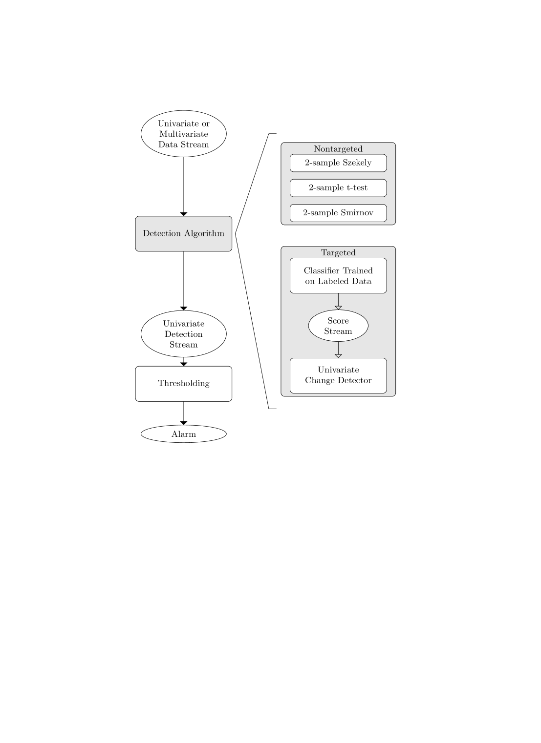
Figure 1: Flow chart showing the general structure of a change detector (left) and two versions of detection algorithms — targeted and untargeted (right).

Figure 2: Standard Gaussian density $p_{0}$ (dashed curve) and Gaussian mixture PDF $p_{1}$ (solid), also with zero mean and unit variance.

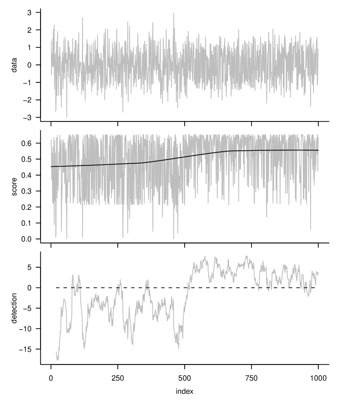
Figure 3: Data stream $x_{i}$ drawn from a standard Gaussian density $p_{0}$ for indices $i=1,\ldots,500$ and from the Gaussian mixture $p_{1}$ of Fig. 2 for $i=501,\ldots,1000$ (top); corresponding score stream $s_{i}$ (middle); and corresponding detection stream $d^{\,lik}_{T}$ with $C=20$ (bottom). The black curve in the middle plot is a smooth of $s_{i}$ obtained by locally weighted regression [3]. The dashed line in the bottom plot indicates the natural break between favoring $p_{0}$ or $p_{1}$ in a log likelihood ratio test.

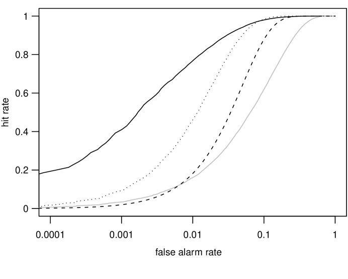
Figure 4: ROC curves for a targeted detector based on $d^{\,lik}_{T}$ (solid dark curve), for an untargeted detector based on the Kolmogorov test statistic (solid gray curve), and for the monkey (dashed curve). The dotted curve is the ROC curve of an unrealizable procedure that uses a Kolmogorov test statistic with a new set of independent data for each recalculation of the statistic within the tolerance window. The sizes of the current set $C$ and of the tolerance window are taken to be 20.

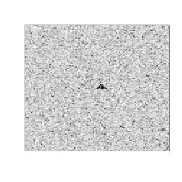
Figure 5: Grey level image of size $100\times 100$ showing uncorrelated standard Gaussian noise, to which has been added an interesting object (the pyramid in the middle, corrupted by noise).

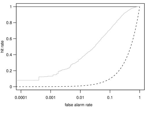
Figure 6: ROC curves for targeted (solid line) and untargeted (gray curve) detectors under the scenario that images contain either just Gaussian noise or an interesting object in the presence of noise (Fig. 5 is an example of the latter case). The dashed curve is for the monkey detector.

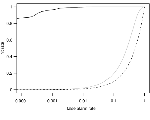
Figure 7: As in Fig. 6, but now under the scenario that some of the images have an uninteresting object (an inverted pyramid).

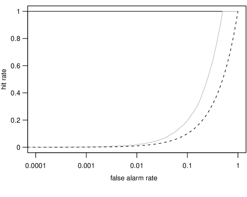
Figure 8: As in Fig. 7, but now with a higher signal-to-noise ratio.

References

- [1] B. Aslan, G. Zech, New test for the multivariate two-sample problem based on the concept of minimum energy, Journal of Statistical Computation and Simulation 75 (2005) 109–119.
- [2] R. Brunelli, Template Matching Techniques in Computer Vision: Theory and Practice, John Wiley & Sons, Chichester, UK, 2009.
- [3] W.S. Cleveland, Robust locally weighted regression and smoothing scatterplots, Journal of the American Statistical Association 74 (1979) 829–836.
- [4] W.J. Conover, Practical Nonparametric Statistics third ed., John Wiley & Sons, New York, 1999.
- [5] T. Fawcett, An introduction to ROC analysis, Pattern Recognition Letters 27 (2006) 861–874.
- [6] A.Y. Kim, C. Marzban, D.B. Percival, W. Stuetzle, Using labeled data to evaluate change detectors in a multivariate streaming environment, Signal Processing 89 (2009) 2529–2536.
- [7] R. Rubinfeld, R. Servedio, Testing monotone high-dimensional distributions, in: Proceedings of the 37th Annual Symposium on Theory of Computing (STOC), 2005, pp. 147–156.
- [8] G.J. Székely, Potential and kinetic energy in statistics, in: Lecture Notes, Budapest Institute of Technology, Technical University, 1989.
- [9] G.J. Székely, E-statistics: energy of statistical samples, Technical Report No. 03–05, Bowling Green State University, Department of Mathematics and Statistics, 2000.
- [10] G.J. Székely, M.L. Rizzo, Testing for equal distributions in high dimension, InterStat, 2004.