The velocity of the dust near the Sun during the Solar Eclipse of March 29, 2006 and sungrazing comets

Abstract

The measurements of the Doppler shifts of the Fraunhofer lines, scattered by the dust grains in the solar F-corona, provides the insight on the velocity field of the dust and hence on its origin. We report on such measurements obtained during the total eclipse of March 29, 2006. We used a Fabry-Pérot interferometer with the FOV of $5.9\degr$ and the spectral resolution of about 5000 to record Fraunhofer spectral lines scattered by the dust of the F-Corona. The spectral region was centered on the Mg i $5172.69\mathrm{\AA}$ line. The measured line-on-sight velocities with the amplitude in the range from -10 to 10 km$\cdot\mathrm{s^{-1}}$ show that during our observations the dust grains were on the orbit with a retrograde motion in a plane nearly perpendicular to the ecliptics. This indicates their cometary origin. Indeed, at the end of March, 2006, SOHO recorded several sungrazing comets with the orbital elements close to what was deduced from our measurements. We conclude that the contribution of comets to the dust content in the region close to the Sun can be more important albeit variable in time. We also deduce that the size of the most of the dust grains during our observations was less than 0.1 $\mu$m.

1 Introduction

The work of van de Hulst (1947) established, after an earlier suggestion by Grotrian (as cited by van de Hulst, 1947), that the emission of the solar outer corona, called F-corona after the Fraunhofer lines composing its spectrum, is due to the scattering of the solar light by the dust particles.

In recent decennia it became more clear that the dust component near the Sun cannot be described as a mere extrapolation of the zodiacal light disc with the dust grains orbiting in the plane of the ecliptics and slowly drifting to the Sun under the Poynting-Robertson effect as one could accept in a first approximation.

The measurements of the Doppler shifts of the Fraunhofer lines in the spectrum of the F-corona, first done during the total eclipse of July 31, 1981 by Shcheglov et al. (1987), and the analysis of the derived velocities by Shestakova (1987), indicated that, although most of the dust particles are orbiting in the ecliptic plane, there are also grains orbiting at high values of inclination angle $i$, implying that the region close to the Sun receives a dust contribution from long-period comets. Also, the in situ measurements of the dust particle velocity distribution on board of HELIOS-1 showed the existence of two distinct components in the interplanetary dust, cometary and asteroidal (Grün et al., 1980). Among more recent results, the high frequency of the Sun-grazing comets recorded by SOHO (MacQueen & St. Cyr, 1991) makes also to consider the cometary contribution as important. Furthermore, studies of extrasolar planetary and dust systems showed the existence of Falling Evaporating Bodies, possibly comets (e.g. Beust et al., 1998). This observational progress was followed by a thorough theoretical modelling taking into account complex composition of the dust in the solar vicinity (see Mann et al., 2000, Kobayashi et al. 2008).

It would have been important to obtain further measurements of the line-on-sight (thereafter LOS) velocities of the dust near the Sun to have a better idea of the relative contributions of the cometary and the ecliptic disc dust components and of their possible variation in time. After the first work of 1981, these measurements, to the best of our knowledge, were successfully attempted only once, during the eclipse of July 11, 1991 (Aimanov et al., 1995) confirming the first results.

Here we present new higher quality measurements of the LOS velocity of the dust in the F-corona obtained during the eclipse on March 29, 2006 (see Shestakova et al., 2007, for a preliminary report), and discuss their implications.

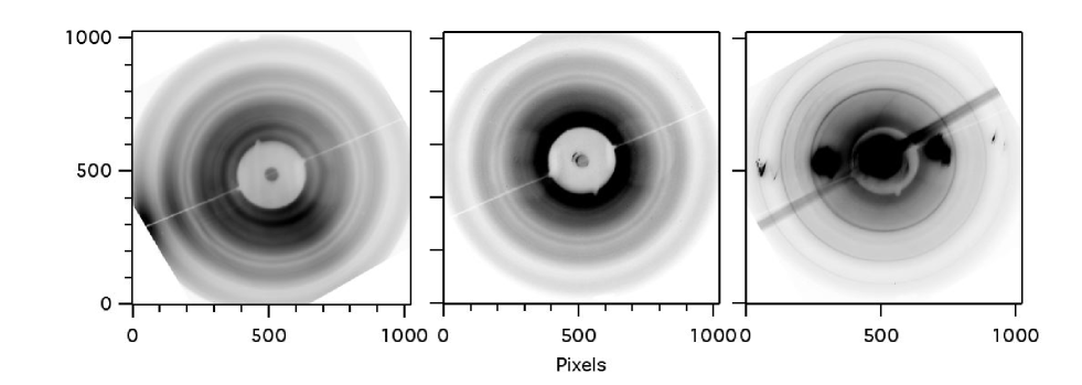
Figure 1: The Fabry-Pérot interferograms of the daylight sky and of the circumsolar region up to elongation $\epsilon\simeq 11$. Here, both axes are in pixels, the platescale is 20.66 arcsec/pix, the FOV $=5.9\degr$. From left to right: a comparison daylight sky frame “D”, the total eclipse frame “E”, and the frame “L” taken at the end of the totality, but already including the green coronal emission line of [Fe XIV] at $\lambda 5302.86\mathrm{\AA}$. The fiducial wire (black line) indicates the East-West direction, the West is to the left along the wire and the North is down. The frames are rotated so that the horizontal axis of the frames coincides with the ecliptic plane. The frames are dark current subtracted. For more details see the text.

2 Observations

The site of the observations was the village of Mugalzhar in the Aktobe region of the Republic of Kazakhstan, at $\phi=48\degr 35\arcmin$ and $\lambda=58\degr 27\arcmin$, situated in the middle of the totality band. According to our calculations, the beginning of the total eclipse was at UT 11h 32m 40, its end at 11h 35m 30s, and the duration of the total phase was 170 s. The Sun was at $27\aas@@fstack{\circ}5$ above the horizon. The weather was mostly rainy and windy during the days preceding the eclipse, but on the eclipse day, the sky was clear with no wind and excellent transparency.

We used the same optical set-up as in our previous measurements in 1991 (Shcheglov et al., 1987), i.e. a Fabry-Pérot (hereafter FP) spectrometer with a coronographic mask rejecting the light of the solar corona and thus reducing the background. The entrance lens of 10 cm diameter has its focal plane at the field lense, the latter is followed by a collimator. The FP etalon in series with an order separation filter is placed in the parallel beam close the exit pupil imaged by the field lense. It is followed by a photographic objective and a CCD detector. The latter was an Apogee Alta-10 CCD device with $2048^{2}$ pixels of 14 $\mu$m size. During the data reduction, the frames were binned by $2\times 2$ pixels, so that to avoid any confusion we will refer from now on to the detector format of $1024^{2}$ pixels with the 28 $\mu$m pixel size.

The solar angular radius at the time of the eclipse was $\mathcal{R}_{\sun}=961$ arcsec, the measured on the CCD value was 46.5 pix. This gives the equivalent focal length of 279.4 mm, and the platescale of 20.66 arcsec/pixel. The field of view (FOV) is $5.9\degr$, corresponding to the elongations $\epsilon<11$, however, to reduce the background light, the central region around the Sun, $\epsilon<2.6$, is hidden by the coronographic mask (hereafter, the elongation $\epsilon$ is given in angular solar radii $\mathcal{R}_{\sun}$).

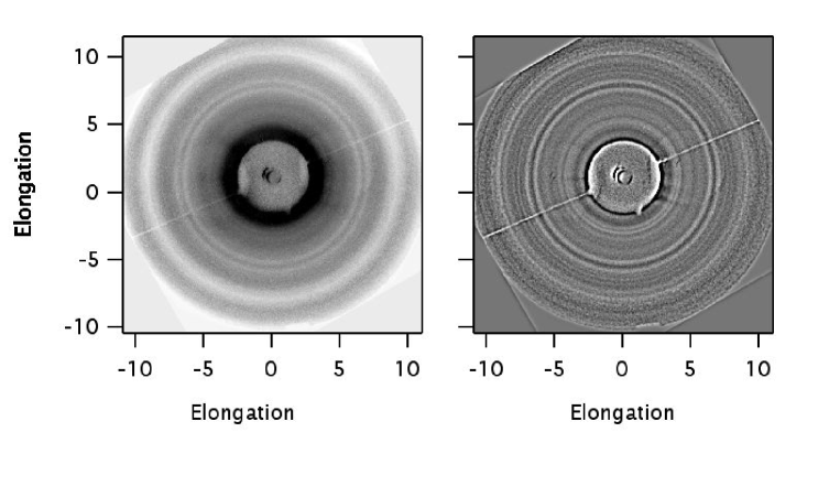
Figure 2: The interferogram of the circumsolar region during the total eclipse in different states of data reduction procedure. Left: after median filtering and dividing on the flat-field as described in the text. Right: The same with the low frequency two-dimensional trend subtracted. The elongation $\epsilon$ is in angular solar radii $\mathcal{R}_{\sun}$.

2.1 Spectro-imaging

We used a mechanically adjustable FP etalon with the free space $\Delta=70\,\mu$m. The order separation filter has the FWHM = $10\,\mathrm{\mathrm{\AA}}$ with the central wavelength close to that of the Mg i line at 5172.69 $\mathrm{\AA}$. In the wavelength space, the set-up is such that a frame includes 4 FP orders. The highest, on-the-axis order $N=\Delta/\lambda$, is at the centre of the frame and is unseen due to the use of the coronographic mask; the orders lower than $N-4$ are outside of the FOV.

The dark subtracted frames obtained during the eclipse are shown in Fig. 1. The left frame, denoted as “D”, is one of the calibration interferograms of the daylight sky, scattered on a white screen, recorded shortly before and after the total phase of the eclipse. The use of the white screen allows a homogenous brightness distribution over the field of view without changing the spectrometer position which remains at the same position as during the total phase. The frame shows concentric rings of the Fraunhofer absorption lines scattered in the terrestrial atmosphere.

The dark circle at the centre of the frame corresponds to the coronographic mask. The dark line corresponds to a fiducial wire indicating the East-West axis, the West to the left along the wire and the North down. For convenience of interpretation, the frames are rotated so that the frames horizontal axis coincides with the ecliptic plane. The frames are dark current subtracted.

The frame “E”in the middle of the Fig. 1 is our main scientific exposure, of 130 s, taken on the circumsolar region during the eclipse. It was started a few seconds after the beginning of the totality and stopped well before its end, so that contamination by coronal or chromospheric lines was avoided. The concentric dark rings are the solar Fraunhofer lines scattered on the dust particles of the F-corona.

Finally, the frame “L”at the right of the Fig. 1, with the exposure time of 20 s was started close to the end of the total phase and lasted a few seconds beyond, so that it caught the light of the solar corona which was just appearing from behind the mask (but not yet the photosphere). On this frame, one can see, additionally to the absorption spectral features of the F-corona, the bright emission rings of the green coronal [Fe XIV] line at $\lambda 5302.86\mathrm{\AA}$. Its wavelength lies far from the centre of the our narrow-band filter, however the emission is so strong that its light passed in the filter transmission wings. The corresponding interference rings well visible in Fig. 1 traced the location of the 3 used Fabry-Pérot orders and gave useful reference points for the data reduction. Its measured $\mathrm{FWHM}=1.2\pm 0.1\mathrm{\AA}$ gives the spectral resolution of the instrument.

The daylight sky interferograms “D” provided the wavelength standard and allowed to eventually measure the Doppler shift of the dust particles of the F-corona, while the interferogram of the coronal green line $\lambda 5302.86\mathrm{\AA}$ allowed to calibrate the spectral geometry of the frames, and in particular to accurately define the rings centre as it will be discussed in Section 3.

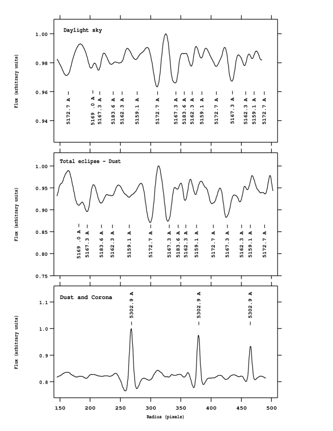
Figure 3: Extracted spectrograms: The flux integrated over the position angle $PA$ in a function of the radius r. Upper plot: The daylight sky, frame “D”; Middle plot: The circumsolar region during the total eclipse, frame “E”; Lower plot: Same but also including the strong coronal emission [$\mbox{Fe\,{\sc xiv}}]\,\lambda 5302.86\mathrm{\AA}$, frame “L”. The relevant Fraunhofer lines and their wavelengths are indicated. Note that there are 3 overlapping spectral orders, they are traced by the [Fe xiv] emission pics.

2.2 Brightness calibration

The weather conditions being excellent and stable, the Fabry-Pérot data were calibrated in brightness relative to that of the solar disc, $B_{\sun}$. Two 0.1 s exposures on the Sun through a combination of a neutral and green filters were taken to the East, at $\epsilon=4.0$, and to the West, at $\epsilon=4.4$ from the Sun position at the total phase of the eclipse. The Sun elevation for the calibration and for the eclipse frames was nearly the same, about $30\degr$. The uncovered surface of the solar disc was 0.94 and 0.25 respectively for the two exposures. Taking this into account, the daylight sky brightness off the eclipse is estimated to has been $4\cdot 10^{-5}B_{\sun}$.

The brightness of the F-corona continuum emission, $B_{F}$, was measured to be $4.1\cdot 10^{-9}B_{\sun}$ at the elongation $\epsilon=4.0$, it was $3.9\cdot 10^{-9}B_{\sun}$ at $\epsilon=4.4$, and $1.7\cdot 10^{-9}B_{\sun}$ for the $\epsilon$ range from 9 to 10. The brightness decrement in the F-corona is in agreement with the results of Koutchmy et al. (1978). Compared to the daylight sky, the F-corona is fainter by a factor of $10^{4}$.

3 Data reduction

The extraction of the Doppler shift of the solar absorption lines out of the Fabry-Pérot interferograms needs a thorough data reduction process. It is worthwhile to be describe here in details.

3.1 Noise and trends handling

After the bias and dark current subtraction, all the frames were $2\times 2$ binned, which increased the signal-to-noise ratio without changing spectral or spatial resolution. The next step was defining all regions meaningless for further reduction, which includes the central dark region corresponding to the coronographic mask, that of the fiducial wire, the part lying out of the field-of-view of the detector and the regions of strong light induced by spurious reflections. The resulting numerically masked area was about 30%.

The “hot”, “cold” and “dead” pixels were cleaned out using a median filter. The visual analysis showed that the “clouds” of defective pixels did not exceed a region of 10-12 pixels a size. We used therefore a non-linear circular filter covering 31 neighbour pixels (i.e. 2n+1, where n is the maximum scale of “clouds”). The correction was applied only to the pixels with the count exceeding 20% of the median value. The number of corrected pixels was less than 4% on the eclipse frames and less than 0.5% on the calibration frames.

For convenience of interpretation, all frames were then rotated so that the horizontal axis coincides with the ecliptic plane.

The next step was the flat-fielding. Usually, it is done by a straightforward division by a averaged flat-field frame with a subsequent masking of the pixels resulting from the division by zero or close to zero values. We decided to optimize this operation by adding a small constant to the flat-field frame. This is similar in its spirit to the Tikhonov regularisation of ill-defined inverse problems. The value of the constant was defined by analysing the histogram of the counts of the flat-field frame. The aim of this operation is to keep moderate, or negligible, the change induced in the signal-to-noise ratio. Thus, the division on the flat-field does not change the structure of the frames and avoids a useless addition of a noise.

Further, we measured the two-dimensional low frequency trend of the resulting frames in order to subtract it and to keep only useful spectro-spatial variations. It was done by using iteratively a linear circular moving average filter. The best filter diameter and the number of iterations were searched by trials in such a way that the frame with the subtracted 2D trend would still keep the structures on a 10-15 pixels scale, which is that of the recorded Fraunhofer lines. The best filter had the diameter of 13 pixels, covering 137 closest pixels, and the best number of iterations was 4. Higher the number of iterations, closer the iterative filter to a linear gaussian smoothing filter, $exp[-(x{{}^{2}}+y{{}^{2}}/(2\sigma_{g}^{2})]$, where $\sigma_{g}$ defines the degree of the smoothing. The advantage of using an iterative filter is the possibility to control the achieved smoothness by limiting the number of iterations.

We tried square and rectangular moving average filters, however they give rise to spur line-like features. We also applied the methods of high and low enveloping curves, but it did not give better results.

The FP interferogram after median filtering and subtraction of the 2D low frequency trend is shown in Fig. 2.

Finally, the data were passed through the gaussian filter with $\sigma_{g}=1.3$ pixels, or $FWHM\approx 3$ pixels which is close to the measured $FWHM$ of the point-spread function of the experiment.

Table 1: Spectral lines identification.

Radius	Elongation $\epsilon$	Wavelength	Element
(pixels)	($\mathcal{R}_{\sun}$)	$\lambda(\mathrm{\AA}$)
182	3.92	5168.91+5169.04	Fe i + Fe ii
196	4.22	5167.33	Mg i
220	4.72	5183.62	Mg i
238	5.12	5162.28	Fe i
266	5.72	5159.06	Fe i
298	6.40	5172.69	Mg i
328	7.06	5167.33	Mg i
344	7.40	5183.62	Mg i
358	7.68	5162.28	Fe i
374	8.04	5159.06	Fe i
402	8.64	5172.69	Mg i
425	9.14	5167.33	Mg i
448	9.64	5162.28	Fe i
460	9.88	5159.06	Fe i
485	10.42	5172.69	Mg i

Table 2: Areas used for the Doppler shift measurements.

Elongation range	Mean $\epsilon$	Lines used
3.12 - 4.09	3.66	5172.7, 5169.0
3.12 - 4.82	4.09	5169.0, 5167.3
4.09 - 4.82	4.52	5167.3, 5183.6
4.82 - 5.63	5.27	5183.6, 5167.3
5.63 - 6.37	6.02	5159.1, 5172.7
6.36 - 7.01	6.71	5172.7, 5167.3
7.01 - 7.74	7.40	5167.3, 5183.6, 5162.3
7.74 - 8.43	8.08	5162.3, 5159.1
8.43 - 9.12	8.77	5172.7, 5167.3
9.12 - 9.63	9.38	5167.3, 5162.3
9.63 - 10.25	9.98	5162.3, 5159.1, 5172.7

3.2 Defining the interferograms centre

In an ideal Fabry-Pérot interferogram, the wavelength $\lambda$ is constant on a circular ring, and varies with its radius as $r{{}^{2}}$. Let $X_{c}$ and $Y_{c}$ denote the coordinates of the centre of the interference rings. Their values depend on many optical parameters, which can vary with temperature and mechanical flexures, so that they must be carefully defined for each frame. After different trials, we found that the most reliable way to measure the centre position was to use a correlation method in the following way.

Let us denote $z=r^{2}$. We adopt a first guess of the centre coordinates $X_{0}$ and $Y_{0}$, and divide the frame on two sub-frames, left and right, symmetrically with the respect to $X_{0}$. For each sub-frame, we compute counts vs $z$, which gives us two functions $L(z)$ and $R(z)$ respectively for the left and the right sub-frames. We compute then the correlation of $L$ and $R$ , and vary $X_{0}$. The maximum of the correlation gives the value of $X_{0}$, which is adopted as $X_{c}$. In a similar way, we define the best value of $Y_{c}$, correlating the upper and the lower sub-frames.

Such a correlation measurement can give false and biased results if, for example, there is a strong asymmetry in the intensity of interference patterns. To have an additional check, we applied another method to smaller parts of the patterns, using only arcs of the rings. For a given ring, we take first guess values of $X_{c}$, $Y_{c}$, $r$, and the width of the ring $dr$. Varying the values of $X_{c}$, $Y_{c}$ and $r$, we find the values such that the sum of counts is the less (for absorption lines). To insure a good statistics, the value of $dr$ must be sufficiently large, but without covering neighbor ring patterns. We used values of $dr$ in the range from 2 to 12 pixels. The difference of the centre coordinates defined by this method and that of correlations did not exceed 0.3 pix, which is at the level of the expected uncertainty.

The resulting values of the center coordinates are defined with an accuracy better than 0.3 pix.

3.3 Reduced spectrograms

Once the centre of the interference rings was found, it is convenient to transform the data presentation from cartesian to polar coordinates $(r,\phi)$. The frames were oriented so that the polar angle $\phi$ and the position angle on the sky, $PA$ are the same for all of them. The extracted spectrograms in the form of the flux integrated over all values of the position angle $PA$ in a function of the radius counted from the interferogram centre are plotted in Fig. 3 for the daylight sky, the circumsolar region during the total eclipse and the frame “L” including the coronal $\mbox{Fe\,{\sc xiv}},\lambda 5302.86\mathrm{\AA}$ line. The 3 pics of the coronal emission line trace the 3 Fabry-Pérot spectral orders. The relevant scattered Fe i, Fe ii and Mg i Fraunhofer lines, in absorption, are indicated. Their wavelengths, the values of the ring radius $r$ and the corresponding value of the elongation $\epsilon$ are given in the Table 1. Albeit the used Fabry-Pérot orders overlap, the spectral features, fortunately, are distinct and can be easily identified.

Figure 4: The line-on-sight velocity of the dust $\bar{V}_{\epsilon}$ vs the elongation $\epsilon$; $\bar{V}_{\epsilon}$ is the average over all range of the position angle $PA$.

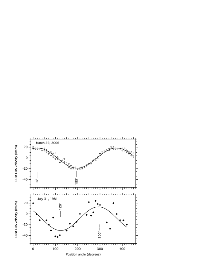
Figure 5: The line-on-sight velocity of the dust averaged over the studied range of elongations, $\bar{V}_{PA}$, vs the position angle $PA$ on March 29, 2006 (upper plot) and on July 31, 1981 (lower plot) together with the fitted $sinus$ curves. For 2006, the triangle marks indicate measurements using two different daylight sky interferograms. The values for the $PA$ range $360\degr-450\degr$ were added for convenience, they merely repeat those for $0-90\degr$. The $PA$ values of the extrema of the fitted to $V_{d}$ $sinus$ curves are given. For the circular orbits lying strictly in the ecliptic plane, the extrema should be at $90\degr$ and $270\degr$.

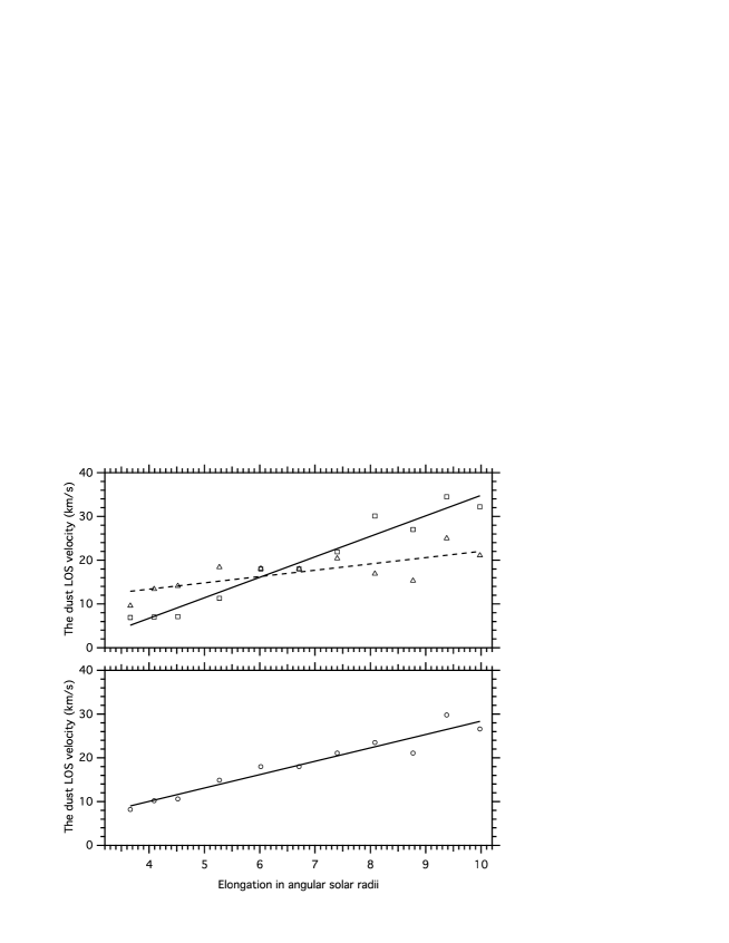
Figure 6: Upper plot: The difference $V_{orb}=V-\bar{V}_{\epsilon}$ vs the elongation $\epsilon$ in the directions of $PA=15\degr$ (rectangles) and $PA=195\degr$ (triangles) and the corresponding linear fits. The values of $V$ are the average over $\pm 30\degr$ wide sectors, they are given in absolute values. The actual sign is positive in the first direction and negative in the second one. Lower plot: The average of the two and the linear fit to it, $V_{orb}=-2.2+3.1\epsilon$

3.4 The line-on-sight velocity of the dust.

The Doppler shift between the eclipse and the daylight spectrograms was measured by cross-correlation. The corresponding dust LOS velocity $V$ writes:

$$V=\frac{c\Delta_{r}^{2}}{2f{{}^{2}}}$$ (1)

or, substituting the numerical values:

$$V=\frac{3\times 10^{6}\times 0.028{{}^{2}}\times\Delta_{r}^{2}}{2\times 86.65{{}^{2}}}=0.01566\times\Delta_{r}^{2}$$ (2)

where $f=86.55$ mm is the focal distance of the camera objective, 0.028 mm is the pixel size, $\Delta_{r}^{2}=r_{e}^{2}-r_{sky}^{2}$, where $r_{e}$ and $r_{sky}$ are the radii in pixels respectively for the eclipse and daylight sky frames. The pixels convert to the elongation $\epsilon$ given that $\mathcal{R}_{\sun}=46.5$ pixels.

The sampling in elongation $\epsilon$ and in position angle $PA$ was as follows. We used intervals of $\epsilon$ as given in Tab. 2 choosing their spanning as regular as possible in a function of the useful spectral lines. The full range of $PA$ was simply divided on 36 sectors $20\degr$ wide each.

For convenience of the analysis, we computed two kinds of average velocities, $\bar{V}_{\epsilon}$, which is the average over all values of $PA$, and $\bar{V}_{PA}$, which is the average over all values of the elongation $\epsilon$.

The value $\bar{V}_{\epsilon}$ is the function of $\epsilon$ only; it is plotted in Fig. 4. If the LOS velocities of the dust grains are distributed in a central symmetry with the respect to the Sun, as it is expected for a pure circular motion, then $\bar{V}_{\epsilon}$ is 0; if not, it reflects the presence of a radial motion, an infall or outflow, at this particular value of $\epsilon$. The Fig. 4 shows that radial motions with velocities about $10\,\mathrm{km}\cdot\mathrm{s}^{-1}$ or less might be present at $\epsilon=4.5$ and $\epsilon\approx 9$, and they are absent, or very small, in between these elongations.

The value $\bar{V}_{PA}$ is a function of the position angle $PA$ only, it is plotted in Fig. 5. It is so particular that we give also for comparison a similar plot from the eclipse on July 31, 1981. For 2006, the triangle marks indicate measurements using two different daylight sky interferograms; their scattering provides an estimate of the uncertainty $\delta\bar{V}_{PA}\simeq 1.6\,\mathrm{km}\cdot\mathrm{s}^{-1}$. The values for the $PA$ range $360\degr-450\degr$ are added for convenience, they merely repeat those for $0-90\degr$. Plotted are also the least squares $sinus$ fits in the form: $\bar{V}_{PA}=k_{1}+k_{2}\cdot sin(k_{3}\cdot PA+k_{4})$. The fit coefficients, for 2006, are as follows: $k_{1}=0.3\pm 0.3$, $k_{2}=18.7\pm 0.3$, $k_{3}=0.01773\pm 0.00016$ and $k_{4}=1.22\pm 0.04$, and for 1981, $k_{1}=8.8\pm 2.5$, $k_{2}=22.0\pm 3.5$, $k_{3}=0.019\pm 0.001$ and $k_{4}=2.4\pm 0.3$.

4 Discussion

Table 3: Orbital elements of sungrazing comets at the end of March, 2006

Comet name	Epoch	Perihelion q	Perihelion	Longitude of	Inclination i
		in $AU$	argument	the node
CK06F050	March 21.96	0.0050	82.38	4.20	144.57
CK06F060	March 23.04	0.0333	56.09	75.03	74.13
CK06F070	March 28.64	0.0050	84.83	3.42	145.72
CK06F080	March 31.10	0.0052	84.02	5.67	144.58

For the prograde orbits being strictly in the ecliptic plane, the minimum LOS velocity $\bar{V}_{PA}$ should be at $90\degr$, i.e. to the East from the Sun, and the maximum $\bar{V}_{PA}$ at $270\degr$, i.e. to the West. The velocity curve measured on July 31, 1981, is close to what is expected from such a motion (with, possibly, a slight difference, the minimum of $\bar{V}_{PA}$ being at $120\degr$ and the maximum at $300\degr$).

As to the $\bar{V}_{PA}$ curve on March 29, 2006, the values of $PA$ of the extrema differ dramatically from what is expected from the prograde motion in the ecliptics, namely the minimum $\bar{V}_{PA}$ is at $195\degr,$ and the maximum is at $15\degr$, meaning a retrograde motion in a plane nearly perpendicular to the ecliptics.

The dust rotating in the prograde direction in the ecliptics is also barely present showing the ”jump” of $\bar{V}_{PA}$ at $PA\simeq 120\degr$ and the symmetric to it another ”jump” at $PA\simeq 300\degr$ (see Fig. 5, upper plot).

Let us verify whether the the LOS velocity behavior agrees with what one would expect from the keplerian motion. This can be seen from the variation of the LOS velocity with the elongation $\epsilon$ at a given $PA$. We assume that the elongation $\epsilon$ of the scattering dust and its heliocentric distance are in a linear relation. We choose the values of $15\degr$ and $195\degr$ for the $PA$, which corresponds to the extrema of $\bar{V}_{PA}$ curve. First of all, the LOS velocities in the considered $PA$’s were averaged within a sector of $\pm 30\degr$ wide, then we subtracted from it the $\bar{V}_{\epsilon}$ value. The resulting “orbital” LOS velocity $V_{orb}(\epsilon)$ is given in Fig. 4 together with the linear fit. The latter gives $\bar{V}_{orb}(\epsilon)=-2.2+3.1\epsilon$ with the $1\sigma$ uncertainty of $\pm 2$ on the additive term and $\pm 0.3$ on the factor. The success of the fit indicates that the motion is indeed keplerian.

Summarizing what is indicated by the $\bar{V}_{PA}$ curve on March 29, 2006, we conclude that the bulk of the dust grains was in a keplerian retrograde motion in a plane nearly perpendicular to the ecliptics. In the inner Solar system, the only objects having this kind of motions are comets.

It happens that indeed around the eclipse date, the SOHO spacecraft recorded a series of sungrazing comets (Mazzucato et al., 2006) of the Kreutz group (Marsden 1967, Sekanina & Chodas 2007). One of them, CK06F050, fell onto the Sun a day before the eclipse, another one, CK06F070, fell a day and a half after the eclipse. For convenience of the reader, the orbital elements as given by Mazzucato et al. (2006), are reproduced in the Tab. 3. It is quite possible that there were also a chain of smaller fragments in between the entities recorded by SOHO, and thus the FOV of our eclipse frame is filled by the dust brought by the Kreutz group comets moving to the Sun on retrograde orbits.

The date of our observations is 8 days past the equinox, so that the line-of-sight to the Sun projects to approximately 8$\degr$ East from that to the vernal point $\Omega$. The longitude of the node of the indicated comets is distant from the $\Omega$ point, according to Tab. 3, by $3\degr-6\degr$. This means that our line-of-sight is inclined with the respect to the line of nodes by only $2\degr-5\degr$. The perihelion argument lies at $84\degr-85\degr$ from the line of nodes.

This means that our image plane is nearly perpendicular to the orbital plane of the comets, and the line-of-sight slides over it.

If the dust grains were strictly confined to the orbital plane, we would see the selected direction indicated by the extrema of the LOS velocities at $PA\approx 55\degr$, which would correspond to the inclination of the parent comet’s orbit of $i=145\degr$. But our data indicate a different axis for the extrema velocities, namely $PA\approx 15\degr$, which indicates $i=105\degr$, i.e. the orbital plane of the dust grains is turned with respect to that of the comets by $40\degr$. The orbital plane cannot change under the gravitational force. Hence, we have to assume another reasons, the effect of the magnetic field on electrically charged dust particles being the most plausible. It follows that the size of particles is quite small, which, in turn, suggests their cometary origin. According to the detailed models of the dust grains dynamics near the Sun by (Krivov et al., 1998) and (Mann et al., 2000), the Lorentz force dominates the gravity for the dust grains smaller than 0.1 $\mu$m i size, and, as show their numerical simulations Mann et al. (2000), the orbits of such grains get randomized which is not th case for the grains with size larger than 0.1 $\mu$m. Interestingly, for grains with the size smaller than 0.01 $\mu$m, the ratio charge-to-mass may be so high that they can be accelerated outward by the interaction with the solar wind as shows their detection by STEREO experiment Meyer-Vernet et al. (2009).

A more detailed modelling of the presented data, taking into account the scattering geometry, dynamics, the density and size distributions of the dust grains, would be highly desirable to quantify further the dust physical properties near the Sun, but this is largely beyond the scope of the present article.

5 Conclusions

The reported here measurements of the Doppler shifts of the Fraunhofer lines, scattered by the dust grains in the solar F-corona, show that at the date of our observations the dust grains were on the orbit with a retrograde motion in a plane at $i\approx 105\degr$, i.e. nearly perpendicular to the ecliptics. This points to their cometary origin. Indeed, at the end of March, 2006, SOHO recorded several sungrazing comets with the orbital elements close to what was deduced from our measurements. We conclude that the contribution of comets to the dust content in the region close to the Sun can be important albeit variable in time. This contribution can explain the already noticed change of the dust distribution from one in the axial symmetry far from the Sun to that in the central, or may be spherical, symmetry Mann et al. (2000).

We also derive that the observed plane of the dust grains orbit is slightly different from that of the parent comet(s), which indicates that the size of grains is small, less than 0.1 $\mu$m, so that they are deviated from the initial orbit by the Lorentz force. This also means that the observed dust grains were released by the comet(s) shortly before our observations.

The importance of comets in a circumstellar environment is general, let us recall e.g. the “Falling Evaporating Bodies” recorded in the spectra of $\beta$ Pic (e.g. Beust et al., 1998). It would be interesting to investigate whether they can provide a sufficient transport of the dust grains between far and close environments of the central star, and to contribute to the dissemination of crystallized material in the recently detected exozodiacal dust discs (Absil et al., 2006, 2009). For a more detailed discussion on the possible role of comet see also Augereau (2009) and references therein.

6 Acknowledgments

We are indebted to many persons who helped to make these measurements possible. A. Dubovitskiy, G. Minasiantz, M. Bayiliev insured the transportation of the instrument and helped with its set-up at the site of the eclipse. A. Didenko provided the Apogee CCD camera, T. Hua supplied a high quality filter on the Mg i line used in this work. We benefited from useful discussions with E. le Coarer, T. Bonev, V. Golev, A.-M. Lagrange, J.-C. Augereau. The expedition to the site of the solar eclipse was funded by the Kazakh National Space Agency and Laboratoire d’Astrophysique de Grenoble (UMR 5571 of the CNRS and Université Joseph-Fourier), the work on the data analysis became possible thanks to the EGIDE administrated ECO-NET grant 18837 - XG of the French Ministry of Foreign Affaires.

References

- Absil et al. (2006) Absil, O., di Folco, E., Ménard, A., et al. 2006, A&A, 452, 237
- Absil et al. (2009) Absil, O., Mennesson, B., Le Bouquin, J., et al. 2009, ApJ, 704, 150
- Aimanov et al. (1995) Aimanov, A. K., Aimanova, G. K., & Shestakova, L. I. 1995, Astronomy Letters, 21, 196
- Augereau (2009) Augereau, J. 2009, in SF2A-2009: Proceedings of the Annual meeting of the French Society of Astronomy and Astrophysics, held 29 June - 4 July 2009 in Besançon, France. Eds.: M. Heydari-Malayeri, C. Reylé and R. Samadi, p.301
- Beust et al. (1998) Beust, H., Lagrange, A., Crawford, I. A., et al. 1998, A&A, 338, 1015
- Grün et al. (1980) Grün, E., Pailer, N., Fechtig, H., & Kissel, J. 1980, Planetary & Space Science, 28, 333
- Kobayashi et al. (2008) Kobayashi, H., Watanabe, S., Kimura, H., & Yamamoto, T. 2008, Icarus, 195, 871
- Koutchmy et al. (1978) Koutchmy, S., Stellmacher, G., Koutchmy, O., et al. 1978, A&A, 69, 35
- Krivov et al. (1998) Krivov, A., Kimura, H., & Mann, I. 1998, Icarus, 134, 311
- MacQueen & St. Cyr (1991) MacQueen, R. M. & St. Cyr, O. C. 1991, Icarus, 90, 96
- Mann et al. (2000) Mann, I., Krivov, A., & Kimura, H. 2000, Icarus, 146, 568
- Marsden (1967) Marsden, B. G. 1967, AJ, 72, 1170
- Mazzucato et al. (2006) Mazzucato, M., Hoffman, T., Matson, R., et al. 2006, Minor Planet Electronic Circulars, 2006-K10
- Meyer-Vernet et al. (2009) Meyer-Vernet, N., Maksimovic, M., Czechowski, A., et al. 2009, Solar Phys., 256, 463
- Sekanina & Chodas (2007) Sekanina, Z. & Chodas, P. W. 2007, ApJ, 663, 657
- Shcheglov et al. (1987) Shcheglov, P. V., Shestakova, L. I., & Aimanov, A. K. 1987, A&A, 173, 383
- Shestakova (1987) Shestakova, L. I. 1987, A&A, 175, 289
- Shestakova et al. (2007) Shestakova, L. I., Rspaev, F. K., Minasyants, G. S., Dubovitskiy, A. I., & Chalabaev, A. 2007, Odessa Astronomical Publications, 20, 203
- van de Hulst (1947) van de Hulst, H. 1947, Ap. J., 105, 471