Exploring extra dimensions through observational tests of dark energy and varying Newton’s constant

Abstract

We recently presented a series of dark energy theorems that place constraints on the equation of state of dark energy ($w_{\rm DE}$), the time-variation of Newton’s constant ($\dot{G}$), and the violation of energy conditions in theories with extra dimensions. In this paper, we explore how current and future measurements of $w_{\rm DE}$ and $\dot{G}$ can be used to place tight limits on large classes of these theories (including some of the most well-motivated examples) independent of the size of the extra dimensions. As an example, we show that models with conformally Ricci-flat metrics obeying the null energy condition (a common ansatz for Kaluza-Klein and string constructions) are highly constrained by current data and may be ruled out entirely by future dark energy and pulsar observations.

I Introduction

Beginning with the work of Kaluza and Klein KK1 ; KK2 ; KK3 and continuing today with string theory and M-theory, extra dimensions have been a common feature of unified theories. The basic notion is that the observed 3+1-dimensional universe is actually described by a general relativistic theory in a space-time with one or more extra compactified dimensions. If the compactification scale is much greater than 1 TeV (or $<<10^{-16}$ cm), laboratory experiments, even at the Large Hadron Collider, are unable to uncover direct evidence of extra dimensions.

In this paper, though, we show how measurements of the equation of state of dark energy ($w_{\rm DE}$) and the time variation of Newton’s constant $\dot{G}/G$ can be used to test or rule out the existence of extra dimensions for large classes of models independent of the compactification scale. This surprising power to discriminate among extra-dimensional models derives from a set of “dark energy theorems,” first described in Wesley:2008de ; Wesley:2008fg ; Steinhardt:2008nk .

The theorems are based on the observation that the expansion of the usual three large dimensions tends to cause extra dimensions to vary with time, which, in turn, causes a change of $w_{\rm DE}$ and $G$ in the corresponding 4d effective theory. These changes can be avoided in a decelerating universe by introducing conventional interactions strong enough to keep the sizes of the extra dimensions fixed. However, the dark energy theorems show that, once the universe starts to accelerate, conventional interactions satisfying the classical (strong, weak and null) energy conditions no longer suffice no matter the size of the extra dimensions. Many well-motivated extra-dimensional models satisfy one or more of the energy conditions. For these large classes, the dark energy theorems, combined with the observed acceleration rate, can be used to compute the predicted time-variation of $w_{\rm DE}$ and $G$ for given model parameters. As illustrated below, current measurements are already strong enough to rule out a substantial range of model parameters. The more exciting prospect is anticipated improvements in the measurement of $w_{\rm DE}$, as described by the Dark Energy Task Force (DETF), and of $\dot{G}/G$, as constrained by pulsar timing, that can test or rule out whole classes of extra-dimensional models.

The dark energy theorems were derived for the general case of $k$ extra spatial dimensions, but the predictions depend on $k$. For the purposes of illustration, we focus in this paper on the well-motivated class of 9+1-dimensional theories ($k=6$) with a conformally flat Ricci (CRF) metric and satisfying the null energy condition (NEC) – theories commonly used in string- and M-theoretic phenomenological and cosmological models. In Ref Steinhardt:2008nk , we showed that this class of models is inconsistent with the standard $\Lambda$CDM model which has $w_{\rm DE}=-1$. In fact, the dark energy theorems show that, the closer $w_{\rm DE}$ is to $-1$, the more rapidly the extra-dimensional volume and, hence, $G$ must vary. Furthermore, if the theory contains no mechanism for violating the null energy condition, $w_{\rm DE}$ cannot remain close to $-1$ for an extended period. This means that improved limits on $\dot{G}$, combined with ever-tightening bounds on the time-variation of $w_{\rm DE}$ from future experiments, can progressively constrain or rule out this entire class of extra-dimensional models.

A corollary of this analysis is that a dark energy mission, even if it fails to find any time-variation of $w_{\rm DE}$ and is consistent with $w_{\rm DE}=-1$, can still be highly informative because it would eliminate well-motivated extra-dimensional models. A second corollary is that a coordinated effort is needed. The ambitious improvements in the measurements of $w_{\rm DE}$ alone, as projected by the DETF, or of $\dot{G}/G$ alone, as estimated from planned pulsar timing surveys, are not sufficient. Each constrains some range of parameter space but leaves some substantial untested range. The two approaches are complementary, though: by pursuing both to some degree, entire classes of extra-dimensional models can be tested and ruled out.

This paper is organized as follows. In Section II, we introduce the conformally Ricci-flat (CRF) class of extra-dimensional models used to exemplify our approach and review the constraints imposed by the dark energy theorems on the total equation of state $w_{\rm tot}$ and Newton’s constant $G$. Here and throughout this paper, the symbol $w_{\rm tot}$ refers to all contributions to the energy density of the universe (matter, radiation, etc.), not just dark energy. The current value is $w_{\rm tot}=-0.74$ based on observations Komatsu:2010fb . We use the symbol $w_{\rm DE}$ to refer to the dark energy component alone.

In Section III, we show how to translate these constraints into predictions for dark energy and pulsar timing experiments. The key results are in Section IV, where we compare the predictions with current measurements and near-future experiments. In particular, we show how current measurements of dark energy and pulsar timing and anticipated improvements can be used to test and perhaps rule out the entire class of models. In Section V, we conclude with a discussion of the generalization to other classes of extra-dimensional models. More details on the constraints on the time-variation of $G$ and the dark energy equation of state in extra-dimensional models are given in the Appendices.

II Dark Energy Theorems and Basic Equations

In this section, we present a brief review of the “dark energy theorems” first described and proven in Wesley:2008de ; Wesley:2008fg ; Steinhardt:2008nk . The theorems impose constraints on extra-dimensional theories in which the four-dimensional effective theory undergoes cosmic acceleration ($w_{\rm tot}<-1/3$). The theorems assume a spacetime metric of the form

$$\text{d}s^{2}=g_{MN}\text{d}X^{M}\text{d}X^{N}=e^{2\Omega(t,y)}g^{\rm FRW}_{\mu\nu}(t,x)\,\text{d}x^{\mu}\text{d}x^{\nu}+h_{\alpha\beta}(t,y)\,\text{d}y^{\alpha}\text{d}y^{\beta}$$ (1)

Here, $\mu,\nu$ … are indices along the four large spacetime dimensions with coordinates $x^{\mu}$, and $\alpha,\beta$ … indices along the $k$ compact dimensions with coordinates $y^{\alpha}$, and $N,M$ … assume values along both compact and noncompact dimensions. In (1), $g^{\rm FRW}_{\mu\nu}$ is a flat Friedmann-Robertson-Walker metric, which we take to be

$$g^{\rm FRW}_{\mu\nu}=-{\cal N}(t)^{2}\text{d}t^{2}+{\cal A}(t)^{2}\delta_{mn}\text{d}x^{m}\text{d}x^{n}$$ (2)

where $m,n$ range over $1...3$. The extra-dimensional metric $h_{\alpha\beta}$ and warp factor $\Omega$ can be time-dependent. For the purposes of illustration, we restrict ourselves in this paper to “conformally Ricci-flat” (CRF) metrics:

$$h_{\alpha\beta}(t,y)=e^{-2\Omega(t,y)}h^{\rm RF}_{\alpha\beta}(t,y)$$ (3)

where $h^{\rm RF}_{\alpha\beta}(t,y)$ has vanishing Ricci scalar, and $\Omega$ is the same warp factor which appears in (1). The CRF metric occurs in many string theory models such as warped Calabi-Yau Giddings:2001yu and warped conifold Klebanov:2000hb constructions (where they are sometimes referred to as conformally Calabi-Yau metrics).

In this work, we further assume that the extra-dimensional matter satisfies the null energy condition (NEC):

$$T_{MN}n^{M}n^{N}\geq 0$$ (4)

for any null vector $n^{M}$, where $T_{MN}$ is the stress-energy tensor. For perfect fluids in four dimensions, the NEC requires that $\rho+P\geq 0$. The NEC is satisfied by scalar fields with canonical kinetic terms (regardless of their potential), de Sitter and anti-de Sitter cosmological constants, $p$-form fields, and positive-tension extended objects. To violate the NEC requires exotic ingredients such as scalar fields with higher-derivative kinetic energy terms or negative-tension extended objects (such as orientifold planes). Very often violation of the NEC leads to ghosts, instabilities, problems with gravitational thermodynamics, and other pathologies.

We will refer to the spectrum of extra-dimensional models having CRF metrics and obeying the NEC as the NEC/CRF family of models. For concreteness, we will take the number of extra dimensions to be $k=6$.

As shown in Wesley:2008de ; Wesley:2008fg ; Steinhardt:2008nk , constraints can be found by considering extra-dimensional theories for which the 4d effective theory is described by Einstein gravity and has $w_{\rm tot}<-1/3$, and, then, following the overall expansion and dilation of the extra-dimensional metric in the extra-dimensional Einstein equations. The time evolution of the higher-dimensional metric can be expressed as the combination of a trace part $\xi$ and a symmetric, traceless shear component $\sigma_{\alpha\beta}$ Wesley:2008de ; Wesley:2008fg ; Steinhardt:2008nk :

$$\frac{1}{2}\frac{\text{d}h_{\alpha\beta}}{\text{d}t}=\frac{1}{k}\xi h_{\alpha\beta}+\sigma_{\alpha\beta}$$ (5)

where $h^{\alpha\beta}\sigma_{\alpha\beta}=0$ and $h_{\alpha\beta}$, $\sigma_{\alpha\beta}$ and $\xi$ are functions of $t$ and $y$. The variable $\xi$ is the local expansion rate of the extra-dimensional space. To measure the overall dilation of the extra dimensions, we define a variable $\zeta_{A}$ by

$$\zeta_{A}=\frac{1}{H}\int e^{A\Omega}\xi\;\sqrt{h}\,\text{d}^{k}y$$ (6)

where $H$ is the four-dimensional Hubble rate, and $A$ is a constant which may be chosen for convenience. Hence $\zeta_{A}$ represents the fractional growth of the extra-dimensional volume per Hubble time, computed using an $A$-dependent measure. For the choice $A=2$, the volume measure in (6) matches the one which determines the four-dimensional Planck mass in warped compactifications. Hence, for this value of $A$ we have

$$\frac{\dot{G}}{G}=-H\zeta$$ (7)

where $G$ is the four-dimensional Newton’s constant, and we dropped the subscript $\zeta_{2}\equiv\zeta$ for economy of notation. When $\zeta$ is nonzero, the volume of the extra dimensions is changing with time, and, hence, the four-dimensional Newton’s constant is changing as well.

The dark energy theorems are derived by assuming that the higher-dimensional matter fields satisfy the NEC Wesley:2008de ; Wesley:2008fg ; Steinhardt:2008nk . By dividing the space-space components of the stress-energy tensor into two blocks corresponding the non-compact and compact directions, two pressure-like parameters can be constructed by taking trace averages over the $3\times 3$ and $k\times k$ blocks of the higher-dimensional metric,

$$p_{3}\equiv\frac{1}{3}g^{mn}T_{mn}\;\;{\rm and}\;\;p_{k}\equiv\frac{1}{k}h^{\alpha\beta}T_{\alpha\beta},$$ (8)

where $m,n$ range over the spatial coordinates $1...3$ and $\alpha,\beta$ range over the extra-dimensional coordinates as in (1). The NEC is violated if either $\rho+p_{3}$ or $\rho+p_{k}$ is less than zero at any space-time point, where $\rho\equiv-{T_{0}}^{0}$ is the higher dimensional energy density; or if the volume weighted average of either is less than zero; or if either of the “A-weighted” averages (the volume-weighted averages of $e^{A\Omega}(\rho+p_{3})$ or $e^{A\Omega}(\rho+p_{k})$) is less than zero for any $A$. By combining the higher-dimensional Einstein equations, expressions can be derived relating the $A$-weighted averages to $\xi$, $\sigma_{\alpha\beta}$, $w_{\rm tot}$, $\Omega$, $k$ and the 4d effective energy density $\rho_{4d}$. The condition that the $A=2$-weighted average of $\rho+p_{k}$ be non-negative can be rearranged into the constraint:

$$\frac{\text{d}\zeta}{\text{d}N}\geq\alpha_{0}+\alpha_{1}\zeta+\alpha_{2}\zeta^{2}$$ (9)

where $N=\ln(a)$ and $a$ is the Einstein frame scale factor. The analogous condition for $\rho+p_{3}$ is

$$\zeta^{2}\leq F$$ (10)

The functions $\alpha_{0}$, $\alpha_{1}$, $\alpha_{2}$, and $F$ depend on $w_{\rm tot}$, the number of extra dimensions $k$ and the type of extra-dimensional metric. For our example with CRF metric and $k=6$ extra dimensions, the strongest observational constraints are found for $A=2$, in which case the value of $\zeta$ is related to the variation of Newton’s constant in four dimensions by (7). Then, the constraint equations (9) and (10) required for the extra-dimensional theory to satisfy the Einstein equations and the NEC become Wesley:2008de ; Wesley:2008fg ; Steinhardt:2008nk :

$$\frac{\text{d}\zeta}{\text{d}N}\geq\zeta^{2}+\frac{3(w_{\rm tot}-1)}{2}\zeta-\frac{9(1+3w_{\rm tot})}{4}$$ (11)

and

$$\zeta^{2}\leq\frac{9(1+w_{\rm tot})}{2}.$$ (12)

With (11) and (12) in hand, we can derive some qualitative consequences of the dark energy theorems for the NEC/CRF family of models. For example, suppose we wish to find a solution for which the four-dimensional Newton’s constant does not vary ($\zeta=0$). With this choice of $\zeta$, the constraint equation (11) can only be satisfied if $w_{\rm tot}\geq-1/3$. Conversely, if the four-dimensional universe is accelerating, then the $\zeta$ must be non-zero and the 4d Newton’s constant must vary.

If $w_{\rm tot}<-1/3$ and the universe is accelerating, $\zeta$ cannot vanish but one might look for cases where $w_{\rm tot}$ and $\zeta$ are constant. Such solutions require that there exists a value of $\zeta$ such that the right-hand side of (11) vanishes. This is only possible when $w_{\rm tot}\geq-5+2\sqrt{5}\simeq-0.53$. We will denote this value of $w_{\rm tot}$ by $w_{\rm trans}$. Thus, a second corollary of the dark energy theorems is that steadily accelerating solutions with constant $\zeta$ are only possible when $w_{\rm tot}\geq w_{\rm trans}$, which in this case corresponds to $w_{\rm tot}\gtrsim-0.53$.

The most striking conclusions of all are reached by considering values of $w_{\rm tot}$ below $w_{\rm trans}$. For $w_{\rm tot}<w_{\rm trans}$, the right-hand side of (11) is positive definite for all values of $\zeta$, so $\zeta$ must evolve with time. Since $\zeta$ is increasing with time, after a finite number of e-foldings the bound encapsulated in (11) and (12) will be violated. Hence there are no steadily accelerating solutions for $w_{\rm tot}<w_{\rm trans}\simeq-0.53$: acceleration with $w_{\rm tot}<w_{\rm trans}$ is necessarily transient.

III Observational constraints and the $w_{0}-w_{a}$ plane

The two constraint equations Eq. (11) and (12) restrict the time-variation of $G$ and $w_{\rm tot}$ for any extra-dimensional model described by a CRF metric and obeying the NEC. In this section, we explain how to express these theoretical constraints as limits on the time-dependence of $w_{\rm DE}$ and, then, how to incorporate observational constraints that can further restrict or perhaps rule out the remaining, theoretically allowed possibilities.

The first step is to parameterize the time-dependence of $w_{\rm DE}$ and $\zeta$. In general, each can have complicated time-dependence. However, in keeping with standard practice, we take $w_{\rm DE}$ to be a simple function of the scale factor $a$ over a range encompassing the present epoch ($0<a<2$ where $a\equiv 1$ today):

$$w_{\rm DE}(a)=w_{0}+(1-a)w_{a}+(1-a)^{2}w_{b}.$$ (13)

The quadratic form is used, rather than the linear DETF parameterization, because the analysis would produce artificially strong constraints for a pure linear dependence.

For $\zeta$, there is only one free parameter that, without loss of generality, can be chosen to be $\zeta_{acc}$, the value when $a=a_{acc}$. For a given $\{w_{0},w_{a},w_{b},\zeta_{acc}\}$, the behavior of $\zeta$ is determined by integrating (9); see Ref.  Wesley:2008fg for details. We define the set of “theoretically allowed” values of $\{w_{0},w_{a},w_{b},\zeta_{acc}\}$ to be those that satisfy all of the following conditions:

• $w_{\rm DE}\geq-1$ for all $a<2$, so that the dark energy component satisfies the null energy condition for all times;

• $w_{\rm DE}\leq 0$ as $a\rightarrow 0$, so the universe is sure to be matter- and radiation-dominated at very early times;

• the constraint equations (11) and (12) are obeyed, so the theory is compatible with the dark energy theorems.

• $\Omega_{DE}$, the ratio of the dark energy density to the critical density equals 0.74, consistent with current observational constraints for $w_{\rm DE}$ near $-1$.

We then project this set of points in the four-dimensional parameter space into the two-dimensional $w_{0}-w_{a}$ subspace. A point $\{w_{0},w_{a}\}$ in this subspace is labeled “compatible with NEC and CRF” if there is at least one choice of $\{w_{b},\zeta_{acc}\}$ such that $\{w_{0},w_{a},w_{b},\zeta_{acc}\}$ satisfies all the conditions above. As shorthand, the set of compatible points is labeled ${\cal C}$. See Figure 1.

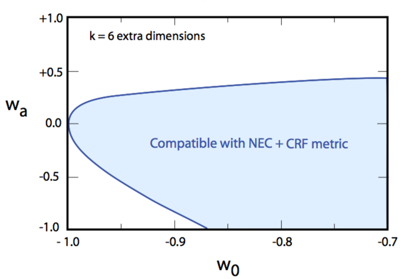
Figure 1: The $(w_{0},w_{a})$-plane where $w_{\rm DE}=w_{0}+w_{a}(1-a)+w_{b}(1-a)^{2}$. The plot shows the boundary of ${\cal C}$, the set of points compatible NEC and CRF for the case of $k=6$ extra dimensions. For any point $\{w_{0},w_{a}\}$ lying within ${\cal C}$, one can find at least one choice of $\{w_{b},\zeta_{acc}\}$ that satisfies the NEC and the dark energy theorems and that is matter-dominated in the past. Conversely, for points outside ${\cal C}$, at least one of these conditions is violated for every choice of $\{w_{b},\zeta_{acc}\}$.

Note that the NEC/CRF compatible region in Figure 1 includes the “de Sitter” point $(w_{0},w_{a})=(-1,0)$, which appears to contradict the claim in Section II that a universe with constant $w_{\rm tot}<w_{\rm trans}$ violates the dark energy theorems. There is no real inconsistency, though: a true 4d de Sitter universe with $w_{\rm tot}=-1$ (or, equivalently, $w_{0}=-1,\,w_{a}=w_{b}=0$) for all time is incompatible with the dark energy theorems. However, it is also possible to choose $w_{b}$ non-zero such that $(w_{0},w_{a})$ is transiently equal to $(-1,0)$ in the present epoch, and yet have $w_{\rm tot}$ increase to values greater than $w_{trans}$ in the past and future, in keeping with the dark energy theorems.

We next add the observational limits on the time-variation of $w_{\rm DE}$ and $G$. For $w_{\rm DE}$, the current limits on $w_{0}$ and $w_{a}$ and the DETF projections for future experiments are used, as reviewed in Appendix B. The current variation of $G$ can be computed from the value of $\zeta$ by

$$\frac{\dot{G}}{G}\bigg{|}_{\rm today}=(-7.4\times 10^{-11}\;\text{yr}^{-1})\times\zeta_{0},$$ (14)

where $\zeta_{0}$ denotes the present value of $\zeta$; the Hubble parameter is taken to be $H=72$ km/s/Mpc; and we have used (7) to relate the variation in $G$ to $\zeta$. The present-day instantaneous constraint on $\dot{G}/G$ is

$$\frac{\dot{G}}{G}=(0\pm 5)\times 10^{-12}\;\text{yr}^{-1}$$ (15)

which results from various experimental studies described in Appendix A. Integrating (7) gives a formula that relates $\zeta(N)$ to the secular variation of $G$ between two times $t_{1}$ and $t_{0}$

$$\frac{G(t_{1})}{G(t_{0})}=\exp\int_{N(t_{1})}^{N(t_{0})}\zeta(N)\,\text{d}N$$ (16)

For the secular variation of $G$, the current bound is

$$\frac{G_{BBN}}{G_{0}}=1.00^{+\,0.20}_{-\,0.16},$$ (17)

where $G_{BBN}$ and $G_{0}$ are the values of $G$ at big bang nucleosynthesis (BBN) and at the present, respectively. Further details about the constraints on secular variation of $G$ may be found in Appendix A.

Using these constraints, we can define a $\chi^{2}$ measure of the agreement between observations and models compatible with the dark energy theorems. The four parameters $w_{0}$, $w_{a}$, $w_{b}$ and $\zeta_{acc}$ suffice to predict the time variation of $w_{\rm DE}$ and $\dot{G}/G$. Then, $\chi^{2}$ as a function of these four variables is

$$\chi^{2}(w_{0},w_{a},w_{b},\zeta_{acc})=\left(\frac{w_{p}+1}{\delta w_{p}}\right)^{2}+\left(\frac{w_{a}}{\delta w_{a}}\right)^{2}+\left(\frac{\dot{G}/G}{\delta[\dot{G}/G]}\right)^{2}+\left(\frac{G_{BBN}/G_{0}-1}{\delta[G_{BBN}/G_{0}]}\right)^{2},$$ (18)

where $\delta w_{0}$, $\delta w_{a}$, … are 1$\sigma$ uncertainties, and $w_{p}$ is the value of $w_{\rm DE}$ at the “pivot” red shift $z_{p}=0.3$. We introduce $w_{p}$ because the DETF convention expresses experimental constraints in terms of $w_{0}$ and $w_{p}$, as described in Appendix B. In terms of our model parameters, $w_{p}$ is given approximately by

$$w_{p}=w_{0}+0.231w_{a}+0.0533w_{b}$$ (19)

In our definition of $\chi^{2}$, we have assumed that future observational data returns a result that best fits $(w_{0},w_{a})=(-1,0)$ in the $w_{0}$-$w_{a}$ plane, and null results for instantaneous and secular variation of $G$, albeit with some uncertainty in these values. We assume the future data differs from current data only in its progressively tighter error bars.

We have found it useful to reduce the full four-variable $\chi^{2}$ function (18) to one which depends on only two variables: $w_{0}$ and $w_{a}$. We define this two-variable $\chi^{2}$ function as the minimum value of the full $\chi^{2}$ function (18) over all $(w_{b},\zeta_{acc})$ in the compatibilty region ${\cal C}$, for the given $(w_{0},w_{a})$. Formally,

$$\chi^{2}(w_{0},w_{a})\equiv\underset{(w_{b},\zeta_{acc})}{\text{min}}\;\chi^{2}(w_{0},w_{a},w_{b},\zeta_{acc}),$$ (20)

where the minimization is understood to be over all $(w_{b},\zeta_{acc})$ such that $(w_{0},w_{a},w_{b},\zeta_{acc})\in{\cal C}$. If we were estimating the values of model parameters, it would be more appropriate to marginalize over $w_{b}$ and $\zeta_{\rm acc}$ than to seek the minimum $\chi^{2}$. However, we want to determine whether any model compatible with the dark energy theorems can also be consistent with future high-precision experiments which give results supporting a cosmological constant and with no time-variation in $G$. Since we are not interested in the specific value of any of our model parameters, but instead in the quality of the best fit, $\chi^{2}$ minimization is more appropriate than marginalization. In the following section, we use the methodology described here to compute $\chi^{2}(w_{0},w_{a})$ based on current and near-future observational constraints.

IV Results

In the previous section, the dark energy theorems were shown to forbid equation of state parameters $(w_{0},w_{a})$ that lie outside region ${\cal C}$ in Fig. 1. In this section, we consider how observational constraints on $w_{\rm DE}$ and $\dot{G}/G$ can further limit and perhaps rule out region ${\cal C}$ itself and, hence, the entire family of NEC/CRF models. Current data is consistent with $w_{\rm DE}=-1$ and $\dot{G}/G=0$; as noted in the previous section, we assume for the purposes of this study that improved measurements will continue to point to the same conclusions about $w_{\rm DE}$ and $\dot{G}/G$ in the future, but with smaller uncertainties. We compute the minimum $\chi^{2}(w_{0},w_{a})$ statistic in (18) based on this assumption. A model will be considered “ruled out if $\chi^{2}(w_{0},w_{a})$ exceeds $3\sigma$ ($99.7\%$ for two parameters).

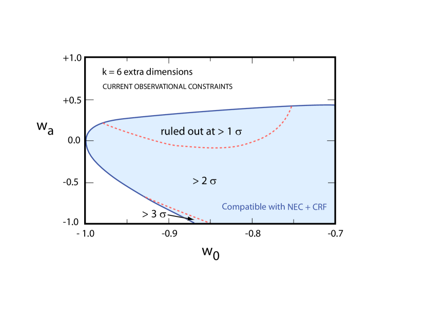
Figure 2: Current constraints on the $(w_{0},w_{a})$ plane for NEC/CRF family of models with $k=6$ extra dimensions. This plot combines present constraints on both dark energy parameters and $\dot{G}$, derived using the techniques described in the manuscript. The contours are generated by choosing the model which best agrees with experimental constraints amongst all models which obey the conditions of the dark energy theorems at each value of $(w_{0},w_{a})$.

Figure 2 illustrates $\chi^{2}(w_{0},w_{a})$ in region $\cal{C}$ based on current observations. Only a small sliver of ${\cal C}$ is ruled out. Figure 3 shows that improving measurements of dark energy only or of $\dot{G}/G$ only is not powerful enough to rule out the entire NEC/CRF family of models. For example, the figure shows that a substantial range of ${\cal C}$ near the “de Sitter” point $(w_{0},w_{a})=(-1,0)$ is still allowed even if the projected sensitivity of the most ambitious and optimistic DETF space-based proposal is achieved. Similarly, a tenfold improvement in $\dot{G}/G$ limits from pulsars, with no dark energy information included, leaves unconstrained a substantial range of ${\cal C}$ with $w_{0}\gtrsim-0.9$. The key point, though, is that the poorly constrained regions of ${\cal C}$ for the two measurements do not overlap, suggesting that a combination of the two can be effective in ruling out all of the NEC/CRF family of models.

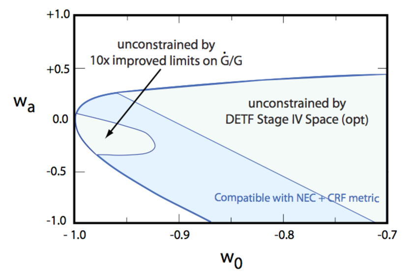
Figure 3: Imposing the constraints from dark energy or $\dot{G}/G$ independently does not constrain the NEC/CRF family of models. Even a very ambitious dark energy measurement, or a significant improvement in pulsar constraints, would leave a region of parameter space which is compatible with the NEC/CRF assumption. Hence, we cannot rule out this family of models by considering these constraints independently.

For example, constraining NEC/CRF models by improving dark energy constraints only and combining them with current $\dot{G}/G$ constraints can rule out the entire NEC/CRF family of models, at the cost of a very ambitious dark energy mission. Figure 4 shows $\chi^{2}(w_{0},w_{a})$ assuming the most ambitious and optimistic DETF concept, a space-based Stage IV proposal. All of ${\cal C}$ is ruled out by more than $3\sigma$. (Stage III and Stage IV ground-based missions may be able to rule out the entire plane if the optimistic DETF projections hold true (at $\sim 3.1\sigma$ and $\sim 3.4\sigma$, respectively), but they would fall short for DETF pessimistic projections.) Although the figure is not shown here, improving constraints on $\dot{G}/G$ only and combining with the current limits on $w_{\rm DE}$ is insufficient to rule out all of ${\cal C}$. In short, improving only one of the two measurements is a difficult approach, at best, for ruling out the NEC/CRF family of models.

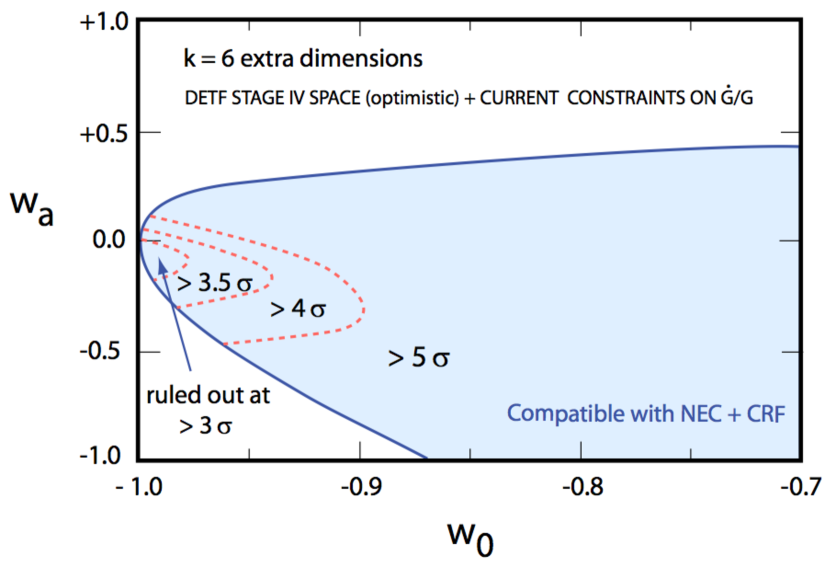
Figure 4: Projected constraints after a Stage IV space-based mission (optimistic) for models obeying the NEC with CRF-type metrics in $k=6$ extra dimensions. With dark energy measurements alone, very ambitious experiments are needed to exclude the full NEC-compatible region, even when current constraints on $\dot{G}/G$ are included. The Stage IV space-based mission is the only DETF scenario which excludes the entire plane to $>3\sigma$ for both pessimistic and optimistic projections.

A less demanding strategy involves modest improvements to measurements of both $w_{\rm DE}$ and $\dot{G}/G$, as illustrated in Figure 5. This figure shows the exclusion regions with DETF Stage II $w_{\rm DE}$ measurements, and only a factor of two improvement in the current value of $\dot{G}/G$. The entire range of ${\cal C}$ can be ruled at $\gtrsim 3.4\sigma$.

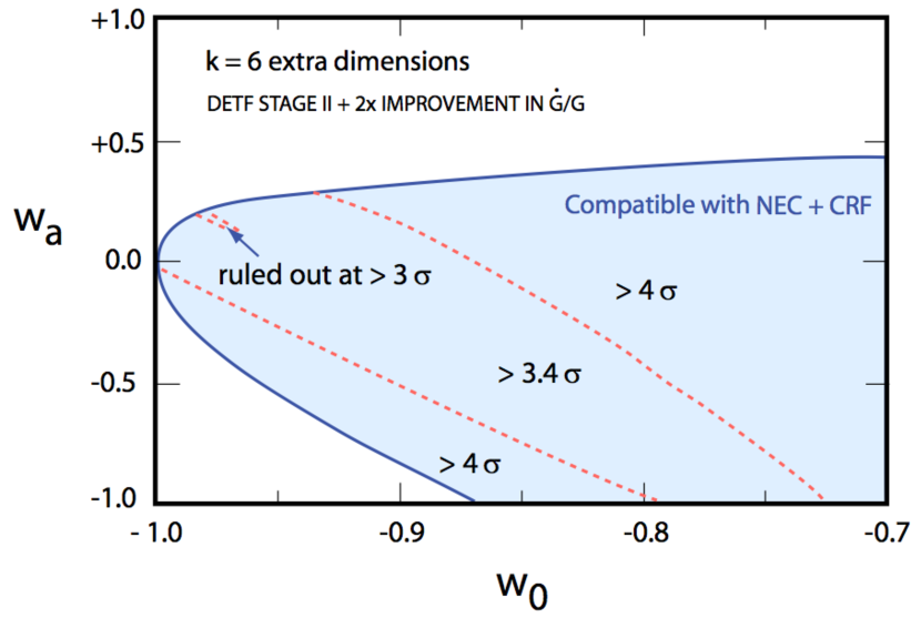
Figure 5: Projected constraints after a DETF Stage II dark energy measurement and a twofold improvement in $\dot{G}/G$ bounds, for models obeying the NEC with CRF-type metrics in $k=6$ extra dimensions. This family of models is excluded at the same level as with a Stage IV dark energy measurement and current $\dot{G}/G$ bounds, hence modest improvements in constraints on both dark energy and $\dot{G}/G$ can do much better than ambitious improvements in dark energy constraints alone.

V Discussion

The results of the previous section demonstrate that it is possible to test and possibly rule out an entire class of extra-dimensional models in a way that does not depend on the size of the extra dimensions. The approach relies on the fact that the expansion of the universe is accelerating today and that acceleration causes the volume of the compactified dimensions to change in cases where the theory satisfies a classical energy condition. Instead of probing the compactified dimensions directly, the approach is to test for the effect of time-variation of the compactified dimensions on $G$ and $w_{\rm DE}$. A key advantage of this approach is that the time variation required by dark energy theorems does not depend on the size of the extra dimensions.

For the purposes of illustration, we have focused on CRF models that obey the NEC because they are common to many string- and M-theoretic constructions. We have demonstrated that current observations allow a significant range of these models, but that improvements in the measurement of $\dot{G}/G$ and $w_{\rm DE}$ anticipated over the next few years can rule them out entirely. To accomplish the task by improved dark energy constraints alone would require the DETF’s most ambitious Stage IV plan combined with current measurements of $\dot{G}/G$.

The most cost-effective approach,, though, is to combine a modest improvement in $\dot{G}/G$ and $w_{\rm DE}$ limits, which can impose constraints tighter than those obtained from a very high-precision dark energy measurement alone. Fig. 6 summarizes how different combinations of improved measurements of $\dot{G}/{G}$ from pulsar timing measurements and dark energy experiments described by the DETF can rule out the entire range of $k=6$-dimensional CRF models obeying the NEC at the $3\sigma$ level or higher.

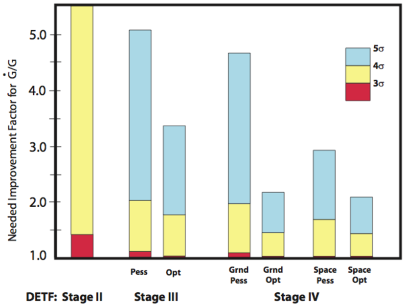
Figure 6: The improvements in $\dot{G}/G$ constraints required to rule out NEC-satisfying models with CRF-type metrics and $k=6$ extra dimensions, as a function of the available dark energy constraints. For each DETF stage, the bars show the improvement in pulsar constraints that would lead to exclusion of this family of models at the 3$\sigma$, 4$\sigma$, and 5$\sigma$ levels. By contrast, this family cannot be ruled out (even at the 1$\sigma$ level) from dark energy information alone, even with constraints from extremely ambitious measurements.

A similar approach can be applied to test other metrics and/or other energy conditions. For example, we have carried out a similar analysis for the family of models in which the extra-dimensional theory satisfies the strong energy condition (SEC) and is described by curved metrics of the form:

$$\text{d}s^{2}=e^{2\Omega(t,y)}g^{\rm FRW}_{\mu\nu}(t,x)\,\text{d}x^{\mu}\text{d}x^{\nu}+h_{\alpha\beta}(t,y)\,\text{d}y^{\alpha}\text{d}y^{\beta}$$ (21)

where $g^{\rm FRW}_{\mu\nu}$ is a flat Friedmann-Robertson-Walker metric; and the extra-dimensional metric $h_{\alpha\beta}$ and warp factor $\Omega$ can be time-dependent. Unlike the CRF family, in (21) we allow the extra-dimensional metric $h_{\alpha\beta}$ to have arbitrary Ricci curvature. This family of models satisfies a set of dark energy theorems that is different from the theorems for NEC/CRF family. We find that, as in the case of the NEC/CRF metrics, the SEC/Curved family of models is not ruled out by current constraints on $w_{\rm DE}$ and $\dot{G}/G$, but DETF Stage II limits combined with current constraints on $\dot{G}/G$ is sufficient to rule out the entire family of models.

We expect to be able to extend our approach to yet more combinations of metrics and energy conditions. Even for the NEC/CRF family of models, it may be possible to derive additional dark energy theorems. The current theorems specify conditions that are necessary to have cosmic acceleration and still satisfy the energy conditions, but they are not sufficient. The current theorems were selected because they are the simplest to prove, as discussed in Ref. Steinhardt:2008nk . However, there may be stronger theorems that combine with observational constraints of $w_{\rm DE}$ and $\dot{G}/G$ to produce much more stringent constraints on extra-dimensional models.

Appendix A Constraints on time-variation of $G$

In Section III we described how the higher-dimensional Einstein equations and energy conditions are distilled into the expressions (9) and (10) for $\zeta\equiv\dot{G}/({G}H)$. Since (9) and (10) are inequalities, they cannot be used to predict a unique value for $\zeta$, but they can place tight constraint the range of values which $\zeta$ can assume. This in turn places constraints on the allowed variation of $G$. The basic technique is illustrated in Figure 7. The plot assumes a cosmological model in which $w_{\rm DE}=-0.8$ and is constant in time. The upper and lower black curves in Figure 7 are $\pm\sqrt{F}$. If the extra-dimensional model obeys the conditions of the theorems, then $\zeta$ must remain in the region between the two outer curves, according to (10). This immediately constrains the present value of $\zeta$, and hence $\dot{G}/G$. For the NEC/CRF family of models considered in this paper, $F=9(1+w_{\rm tot})/2$ today is of order unity, and so this initial constraint tells us that $G$ should vary by no more than order unity per Hubble time.

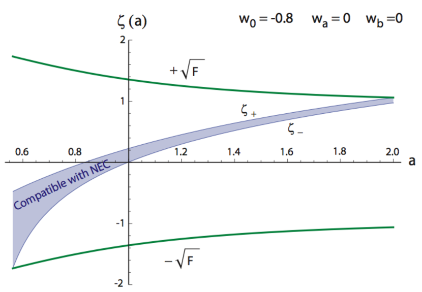
Figure 7: The constraints on $\zeta$ imposed by the dark energy theorem inequalities (9) and (10) for a flat matter-quintessence model with $\Omega_{\rm dark}=0.74$ and $w_{\rm DE}=-0.8$ being constant, for which $w_{\rm tot}$ passes through $-1/3$ at $z=0.78$. The curves are computed for NEC-satisfying models with CRF-type metrics and $k=6$ extra dimensions. The upper and lower curves are the limits $\pm\sqrt{F}$ obtained from (10). The curve $\zeta_{-}$ is the solution obtained by saturating (9) and using the most negative initial value for $\zeta$ allowed by (10). The curve $\zeta_{+}$ is obtained in the same way, but uses the largest possible initial value for $\zeta$ which does not cross over $\sqrt{F}$ by $a=2$. All $\zeta(a)$ trajectories which are compatible with NEC must lie within the central band.

To determine the constraints derived from the differential inequality (9), it suffices to consider trajectories $\zeta_{\pm}$ that saturate the inequality, as illustrated in Figure 7. Since this differential equation is first-order, the trajectories obtained with different initial values of $\zeta$ never cross each other, so trajectories that satisfy the inequalities are bounded by $\zeta_{\pm}$. As a practical matter, we impose initial conditions for $\zeta$ at the beginning of the accelerating epoch, when $w=-1/3$, and integrate $a=2$, figuring that our simple parameterization of dark energy should not be trusted for a much wider range of $a$.

We define $\zeta_{-}$ as the solution to (9) which saturates the inequality and uses the smallest allowed initial value of $\zeta$ when $w_{\rm tot}=-1/3$. By an ”allowed” initial value, we mean one for which the trajectory resulting from integrating (9) never leaves the envelope $\pm\sqrt{F}$ before the end of the integration interval. In some cases, such as the one illustrated in Figure 7, the initial value for $\zeta_{-}$ is at the lower edge of the $\pm\sqrt{F}$ envelope, at $\zeta=-\sqrt{F}$. In other cases, a larger initial value may be necessary to avoid leaving the $\pm\sqrt{F}$ envelope before the end of the integration interval. The function $\zeta_{+}$ is defined in a parallel fashion: it is the trajectory defined by (9) which uses the largest possible initial value of $\zeta$ and does not leave the $\pm\sqrt{F}$ envelope before the end of the integration interval.

Using the two functions $\zeta_{\pm}$ we can put much tighter constraints on the allowed behavior of $\zeta$. The solutions $\zeta_{\pm}$ divide the allowed region between $\pm\sqrt{F}$ into three subregions:

The $-\sqrt{F}<\zeta<\zeta_{-}$ region is forbidden by the energy condition. We can show this by contradiction. Suppose there is a curve $\bar{\zeta}(a)$ which reaches a point $(\zeta_{1},a_{1})$ located in this region but satisfies the conditions of the theorems. Then at the beginning of acceleration, $\bar{\zeta}>-\sqrt{F}$ by (10). By continuity, the curve $\bar{\zeta}(a)$ must have crossed the curve $\zeta_{-}$ at some $a_{\star}<a_{1}$, and in particular gone from above the curve to below. This is a contraction, for at the crossing, the slope of $\bar{\zeta}$ is less than that of $\zeta$, and since $\zeta=\bar{\zeta}$ at the crossing point, (9) could not have been satisfied. A similar argument applies to $\zeta_{+}<\zeta<+\sqrt{F}$. Therefore any function $\bar{\zeta}$ which satisfies both inequalities (9) and (10) is confined to the region $\zeta_{-}\leq\zeta\leq\zeta_{+}$. Using the relationships (7) and (16), this constraints on $\zeta$ translate into constraints on the allowed values of the ratio between $G$ at the beginning of the accelerating epoch and today, and the present value of $\dot{G}/G$.

For example, in the case shown in Figure 7, the present values of $\zeta_{-}$ and $\zeta_{+}$ today are approximately $5.87\times 10^{-3}$ and $2.26\times 10^{-1}$, corresponding to

$$-1.68\times 10^{-11}\;\text{yr}^{-1}\leq\frac{\dot{G}}{G}\bigg{|}_{\rm today}\leq-4.33\times 10^{-13}\;\text{yr}^{-1}$$ (22)

where the upper limit comes from $\zeta_{-}$ and the lower limit from $\zeta_{+}$. This entire range is essentially consistent with the current experimental limits (15) at roughly $3\sigma$. There is a gap between the upper limit and zero, which means that $G=$ constant is not consistent with the NEC/CRF family of models. This gap could be explored at $3\sigma$ with a significant improvement of the instantaneous $\dot{G}/G$ constraints (15) by roughly a factor of $\sim 35$. The limits from secular change in $G$ over the accelerating epoch are

$$0.678\leq\frac{G_{BBN}}{G_{0}}\leq 0.929$$ (23)

where the lower limit corresponds to $\zeta_{+}$ and the upper one to $\zeta_{-}$.

A.1 Observational constraints on the instantaneous variation of $\dot{G}/G$

There is a long history of searches for variation of Newton’s constant $G$ (for a recent review, see Uzan:2002vq ). In recent years interest in measuring the variation of $G$ (as well as other fundamental constants) has been driven by ideas in higher-dimensional unification and modified theories of gravity which may explain cosmic acceleration.

To be useful in our analysis, it is important that we use constraints on the time-variation of $G$ that do not make specific assumptions about the functional form of the time-dependence. For example, some constraints on the instantaneous variation of $\dot{G}/G$ are obtained by assuming $G(t)\sim t^{\beta}$. For some special functional forms, such as this, one can obtain very strong observational limits on $\dot{G}/G$ by applying constraints on the value of $G$ in distant past, (e.g., from big bang nucleosynthesis). We cannot use such constraints, because there is no guarantee that the variation of $G$ predicted by the dark energy theorems will follow any particular simple form. Similarly, we cannot use constraints based on stellar evolution that average over one or more Gyrs to place a limit on the current instantaneous variation of $G$ since the current value of $\dot{G}/G$ may be very different from the average over the last Gyr.

We also must avoid constraints which depend on a particular modification of gravity. By assuming a particular gravitational theory, it is sometimes possible to obtain tight constraints on theory parameters by other measurements, and then use these parameters to derive a constraint on the current value of $\dot{G}/G$. One common example is to assume Brans-Dicke theory: constraining the Brans-Dicke parameter $\omega_{\rm BD}$ by, for example, measuring the Shapiro delay can be used to provide an indirect constraint on the current variation of $G$. We must discard such constraints because the assumption of a particular gravitational theory is always in the background.

The ideal constraints on the current variation of $G$ are those which use data over very short timescales – such as a few decades – that are extremely small in comparison with cosmological timescales, and make minimal assumptions about the gravitational theory being tested. No test can ever be completely model-independent, but assuming Einstein gravity is a conservative assumption which leaves us at little risk for being misled.

Solar system constraints are ideal for bounding the variation of $G$, due to the short measurement timescales and nearly Newtonian regime. An early constraint on the variation of $G$ from analyzing ranging data to the Viking Mars lander Viking gave a constraint of $\dot{G}/G=(2\pm 4)\times 10^{-12}\;\text{yr}^{-1}$ The dominant source of uncertainty was the modeling of asteroid effects on the orbit of Mars. Using the same data set, but a different asteroid model, others have obtained slightly weaker limits of $|\dot{G}/G|<3\times 10^{-11}\;\text{yr}^{-1}$ Viking2 and $|\dot{G}/G|<1\times 10^{-11}\;\text{yr}^{-1}$ Viking3 , so it is possible that the initial uncertainties may have been underestimated. Measurements using planets in the inner solar system are less sensitive to uncertainties due to the asteroid belt. An early constraint of $|\dot{G}/G|<4\times 10^{-10}\;\text{yr}^{-1}$ Shapiro:1971qy was obtained from radar ranging of Mercury. This has been sucessively refined over the intervening decades ReasShap76 ; ReasShap78 ; Shap90 . Currently, the constraint

$$\frac{\dot{G}}{G}=(0\pm 2)\times 10^{-12}\;\text{yr}^{-1}$$ (24)

follows from an analysis of a combination of ranging data from Mariner 10, Mercury and Venus IPCombo .

Pulsar timing measurements have also obtained very stringent bounds on the instantaneous variation of $G$. In contrast with solar-system tests, post-Newtonian effects in pulsar systems, such as the influence of gravitational binding energy and damping due to the emission of gravitational radiation, cannot be neglected. There are also theoretical uncertainties involving the composition of the bodies in the pulsar system. Usually in these cases one must take a phenomenological approach to obtain reasonably model-independent bounds. One approach relates the anomalous pulse period derivative $\delta\dot{P}$ to the variation of $G$ by $\delta\dot{P}/P=-2\dot{G}/G$. When applied to the Hulse-Taylor pulsar PSR 1913+16, after successive refinements Damour88 ; Damour:1990wz ; Kaspi:1994hp this gives the bound

$$\frac{\dot{G}}{G}=(4\pm 5)\times 10^{-12}\;\text{yr}^{-1}$$ (25)

A similar analysis of the pulsar PSR B1855+09 gives the slightly weaker bound $\dot{G}/G=(-9\pm 18)\times 10^{-12}\;\text{yr}^{-1}$. This bound is somewhat more conservative than the one for PSR 1913+16, since the companion is not a neutron star, hence there are fewer composition-dependent uncertainties.

For our work we adopt the canonical present-day constraint of

$$\frac{\dot{G}}{G}=(0\pm 5)\times 10^{-12}\;\text{yr}^{-1}\quad\text{(this work)}$$ (26)

This uncertainty envelops both the recent constraints (25) from PSR 1913+16 and the inner solar-system tests (24). This is a conservative constraint, for its uncertainty agrees with the pulsar constraint, which is the larger of the two. Furthermore, the mean value is taken to be zero, in agreement with the solar-system tests and with the simplest theoretical hypothesis that $\dot{G}/G=0$ today.

A.2 Observational constraints on the secular variation of $G$

Another set of constraints on variation of $G$ arise from the integrated variation of $G$ over cosmic history. Many of the same caveats for constraints on the instantaneous variation of $G$ apply here as well: use constraints which do not assume a specific functional form for the variation of $G$ with time and which do not make strong model-dependent theoretical assumptions. These constraints bound the ratio between $G_{0}$, the value of $G$ today, and the value of $G$ at an earlier epoch of cosmic history.

The most precise constraints of the variation of $G$ with cosmic time have come from big bang nucleosynthesis (BBN). Changing the value of $G$ changes the Hubble expansion rate during BBN, which affects freeze-out temperatures and the rate of various nuclear reactions. This leads to different predictions for primordial abundances of D, ³He, ⁴He, and ⁷Li. These predictions also depend on the baryon-to-photon ratio $\eta$ and the number of relativistic species during BBN, which is usually parameterized by the number of light neutrino species $N_{\nu}$. Allowing $(G,\eta,N_{\nu})$ to vary led to the early bound of $0.7>G_{BBN}/G_{0}>1.4$ Accetta:1990au . Later, using more recent evidence that $N_{\nu}=3$ and an independent determination of $\eta$ from cosmic microwave background measurements, this bound was refined to Copi:2003xd

$$\frac{G_{BBN}}{G_{0}}=1.01^{+\,0.20}_{-\,0.16}$$ (27)

In this work we take the essentially identical bound

$$\frac{G_{BBN}}{G_{0}}=1.00^{+\,0.20}_{-\,0.16}\quad\text{(this work)}$$ (28)

which differs from (27) by recalibrating the mean value of the ratio to be unity, in accord with the simplest theoretical hypothesis that $G$ has been constant since BBN.

There is an additional assumption which is specific to our analysis. As we describe in more detail in Section III, the dark energy theorems bound the variation of $G$ from the beginning of the accelerating epoch, where $G=G_{acc}$ to the present day, where $G=G_{0}$. There are no precise measurements of $G$ at the transition from deceleration to acceleration, so we will use the ratio of $G_{BBN}/G_{0}$ as a stand-in for the ratio $G_{BBN}/G_{0}$.

Appendix B Constraints on $w_{DE}$

The discovery that the present universe is accelerating Riess:1998cb ; Perlmutter:1998np has triggered theoretical efforts to understand this fact, and experimental searches to better characterize the properties of the dark energy that is presumably responsible (for reviews, see Weinberg:1988cp ; Padmanabhan:2002ji ; Peebles:2002gy ; Copeland:2006wr ). One simple possibility, consistent with all current data, is that the dark energy is a cosmological constant. It is also possible that dark energy is dynamical, so that its equation-of-state parameter $w_{\rm DE}$ varies with time. Present and future experimental data can constrain this possibility. A significant problem with applying these constraints is that they usually depend on a specific choice for parameterizing the variation of $w_{\rm DE}$ with time.

An issue in combining observational constraints and constraints from the dark energy theorems is how to parameterize the time-variation of $w_{\rm DE}$. Some studies of supernova data DiPietro:2002cz ; Riess:2004nr choose a parameterization, first suggested in Cooray:1999da , of the form

$$w_{\rm DE}=w_{0}+w^{\prime}z$$ (29)

where $w_{0}$ is the dark energy equation-of-state parameter today, and $w^{\prime}=\text{d}w/\text{d}z|_{z=0}$. With this parameterization, the constraints $w_{0}=-1.31^{+\,0.22}_{-\,0.28}$ and $w^{\prime}=1.48^{+\,0.81}_{-\,0.90}$ were obtained Riess:2004nr , with the errors in each parameter strongly correlated. If $w_{\rm DE}$ is assumed to be constant, then the constraints $w_{\rm DE}=-1.02^{+\,0.13}_{-\,0.19}$ has been obtained Riess:2004nr . Another choice of parameterization, proposed in Chevallier:2000qy ; Linder:2002et , is

$$w_{\rm DE}=w_{0}+w_{a}(1-a)=w_{0}+w_{a}\frac{z}{1+z}$$ (30)

which assumes dark energy evolution linear in the scale factor $a$. This has been used in some recent supernova analyses Riess:2006fw ; Kowalski:2008ez , along with data from cosmic microwave background (CMB) and baryon acoustic oscillations (BAO). In Ref. Kowalski:2008ez this led to correlated errors on $w_{0}$ and $w_{a}$ of roughly $\pm 0.2$ and $\pm 0.7$, respectively. In the same reference, by a flat universe with $w_{\rm DE}$ constant gives constraints of $w_{\rm DE}=-1.001\pm 0.071\text{(stat)}\pm 0.081\text{(sys)}$.

Analysis of the seven-year Wilkinson Microwave Anisotropy Probe (WMAP) data has also given constraints on dynamical dark energy Komatsu:2010fb . If the equation-of-state $w_{\rm DE}$ is constant, then CMB data alone constrains $w_{\rm DE}=-1.10\pm 0.14$ at $1\sigma$. Allowing the $w_{\rm DE}$ to vary linearly with $a$ gives the constraints $w_{0}=-0.93\pm 0.13$ and $w_{a}=-0.41^{+0.72}_{-0.71}$ at $1\sigma$. Similar results are obtained from the WMAP five-year analysis Komatsu:2008hk .

In this work, we draw from these various analyses, and take today’s value $w_{0}$ of the equation-of-state to be

$$w_{0}=-1.00\pm 0.13\quad\text{(this work)}$$ (31)

The uncertainty is the same as the WMAP seven-year analysis, which compares favorably with the the uncertainties in the supernovae analyses. While the WMAP analysis prefers a central value of which is roughly $1\sigma$ from $w_{0}=1$, we have chosen to fix the central value at $-1$ for the purposes of our analysis, based on the notion that a cosmological constant is consistent with all data sets and is the simplest assumption. For the current constraints only, we have chosen to place no limits on $w_{a}$, since the variety of paremeterizations used in the literature make it difficult to compare this parameter between analyses.

For projections of future dark energy parameter uncertainties, the Dark Energy Task Force (DETF) report Albrecht:2006um is used. This report introduces the simple linear parameterization in (30). However, projected uncertainties are given in terms of two different parameters $(w_{p},w_{a})$. The parameter $w_{p}$ is the value of $w_{\rm DE}$ at the “pivot redshift” $z_{p}\approx 0.3$. The pivot redshift is the redshift at which a specific experiment can determine the value of $w_{\rm DE}(z_{p})$ with minimum uncertainty.

The DETF report defines the potential progression in our observational knowledge in terms of four stages:

• Stage I. Current experiments.

• Stage II. Ongoing experiments related to dark energy.

• Stage III. Near-term, currently proposed projects. Ref. Albrecht:2006um considers ground-based surveys for BAO, cluster lensing, supernovae, and weak lensing.

• Stage IV. Ambitious long-term projects, such as the Large Survey Telescope (LST), Square Kilometer Array (SKA), or Joint Dark Energy Mission (JDEM)

Projections for both pessimistic and optimistic error ellipses in the $(w_{p},w_{a})$ plane are given for Stages II-IV. Furthermore, Stage IV projections are given for both ground-only and space-based Stage IV campaigns.

Table 1: Data scenarios for dark energy measurements. These are taken from the DETF report. We show the scenario name (used in our computer code), the uncertainty $\Delta w_{p}$ in $w_{\rm DE}$ a the pivot redshift, and the uncertainty $\Delta w_{a}$ in $w_{a}$ at the pivot redshift.

Scenario	$\Delta w_{p}$	$\Delta w_{a}$	Notes
node			No dark energy constraints.
currde	$0.13$		Current uncertainty, central $w_{0}=-1$
detfII	$0.045$	$0.66$	DETF Stage II
detfIIIp	$0.031$	$0.36$	DETF Stage III, pessimistic
detfIIIo	$0.025$	$0.23$	DETF Stage III, optimistic
detfIVGp	$0.030$	$0.31$	DETF Stage IV ground, pessimistic
detfIVGo	$0.016$	$0.11$	DETF Stage IV ground, optimistic
detfIVSp	$0.023$	$0.15$	DETF Stage IV space, pessimistic
detfIVSo	$0.015$	$0.12$	DETF Stage IV space, optimistic

A summary of the various data scenarios we consider is given in Table 1.

References

- (1) Nordström, Gunnar. Physikalische Zeitschrift 15 504 506 (1914).
- (2) Kaluza, Theodor. Sitzungsber. Preuss. Akad. Wiss. Berlin. (Math. Phys.) 966 972 (1921)
- (3) Klein, Oskar. Zeitschrift f r Physik a Hadrons and Nuclei 37 895 906. (1926).
- (4) S. W. Hawking and G. F. R. Ellis. The large-scale structure of space-time. Cambridge University Press, 1973.
- (5) D. H. Wesley, arXiv:0802.2106 [hep-th].
- (6) D. H. Wesley, JCAP 0901, 041 (2009) [arXiv:0802.3214 [hep-th]].
- (7) P. J. Steinhardt and D. Wesley, Phys. Rev. D 79, 104026 (2009) [arXiv:0811.1614 [hep-th]].
- (8) E. Komatsu et al., arXiv:1001.4538 [astro-ph.CO].
- (9) G. W. Gibbons, in F. del Aguila, J.A. de Azcárraga, L.E. Ibánez (eds), Supersymmetry, supergravity, and related topics. World Scientific, Singapore, 1985.
- (10) J. M. Maldacena and C. Nunez, Int. J. Mod. Phys. A 16, 822 (2001) [arXiv:hep-th/0007018].
- (11) J. P. Uzan, Rev. Mod. Phys. 75, 403 (2003) [arXiv:hep-ph/0205340].
- (12) R. W. Hellings et. al. Phys. Rev. Lett. 51, 1609 (1983)
- (13) R. W. Hellings et. al. Philo. Trans. R. Soc. London A 310, 227 (1983)
- (14) J. F. Chandler, R. D. Reasenberg, I. I. Shaprio et. al. Bull. Amer. Astro. Soc. 25, 1255 (1993)
- (15) I. I. Shapiro, W. B. Smith, M. B. Ash, R. P. Ingalls and G. H. Pettengill, Phys. Rev. Lett. 26, 27 (1971).
- (16) R. D. Reasenberg and I. I. Shapiro in Atomic Masses and Fundamental Constants, Vol. 5, edited by J. H. Sanders adn A. H. Wapstra (Plenum, New York 1976) p 643.
- (17) R. D. Reasenberg and I. I. Shapiro in On the Measurements of Cosmological Variations of the Gravitational Constant,edited by L. Halperin (University of Florida, Gainsville FL), p. 71
- (18) I. I. Shapiro in General Relativity and Gravitation, edited by N. Ashby, D. F. Bartlett, and W. Wyss (Cambridge University Press, Cambridge, England).
- (19) J. D. Anderson et. al in Proceedings of the 6th Marcel Grossman Meeting on General Relativity, Kyoto, June 1991. Edited by H. Sato and T. Nakamura (World Scientific, Singapore), p. 353
- (20) T. Damour, G. W. Gibbons and J. H. Taylor. Phys. Rev. Lett. 61, 1151 (1988).
- (21) T. Damour and J. H. Taylor, Astrophys. J. 366, 501 (1991).
- (22) V. M. Kaspi, J. H. Taylor and M. F. Ryba, Astrophys. J. 428, 713 (1994).
- (23) F. S. Accetta, L. M. Krauss and P. Romanelli, Phys. Lett. B 248, 146 (1990).
- (24) C. J. Copi, A. N. Davis and L. M. Krauss, Phys. Rev. Lett. 92, 171301 (2004) [arXiv:astro-ph/0311334].
- (25) A. G. Riess et al. [Supernova Search Team Collaboration], Astron. J. 116, 1009 (1998) [arXiv:astro-ph/9805201].
- (26) S. Perlmutter et al. [Supernova Cosmology Project Collaboration], Astrophys. J. 517, 565 (1999) [arXiv:astro-ph/9812133].
- (27) S. Weinberg, Rev. Mod. Phys. 61 (1989) 1.
- (28) T. Padmanabhan, Phys. Rept. 380, 235 (2003) [arXiv:hep-th/0212290].
- (29) P. J. E. Peebles and B. Ratra, Rev. Mod. Phys. 75, 559 (2003) [arXiv:astro-ph/0207347].
- (30) E. J. Copeland, M. Sami and S. Tsujikawa, Int. J. Mod. Phys. D 15, 1753 (2006) [arXiv:hep-th/0603057].
- (31) A. R. Cooray and D. Huterer, Astrophys. J. 513, L95 (1999) [arXiv:astro-ph/9901097].
- (32) E. Di Pietro and J. F. Claeskens, Mon. Not. Roy. Astron. Soc. 341, 1299 (2003) [arXiv:astro-ph/0207332].
- (33) A. G. Riess et al. [Supernova Search Team Collaboration], Astrophys. J. 607, 665 (2004) [arXiv:astro-ph/0402512].
- (34) M. Chevallier and D. Polarski, Int. J. Mod. Phys. D 10, 213 (2001) [arXiv:gr-qc/0009008].
- (35) E. V. Linder, Phys. Rev. Lett. 90, 091301 (2003) [arXiv:astro-ph/0208512].
- (36) A. G. Riess et al., Astrophys. J. 659, 98 (2007) [arXiv:astro-ph/0611572].
- (37) M. Kowalski et al., arXiv:0804.4142 [astro-ph].
- (38) E. Komatsu et al. [WMAP Collaboration], arXiv:0803.0547 [astro-ph].
- (39) A. Albrecht et al., arXiv:astro-ph/0609591.
- (40) D. Huterer and M. S. Turner, Phys. Rev. D 64, 123527 (2001) [arXiv:astro-ph/0012510].
- (41) I. Maor, R. Brustein, J. McMahon and P. J. Steinhardt, Phys. Rev. D 65, 123003 (2002) [arXiv:astro-ph/0112526].
- (42) W. Hu and B. Jain, Phys. Rev. D 70, 043009 (2004) [arXiv:astro-ph/0312395].
- (43) S. B. Giddings, S. Kachru and J. Polchinski, Phys. Rev. D 66, 106006 (2002) [arXiv:hep-th/0105097].
- (44) I. R. Klebanov and M. J. Strassler, JHEP 0008, 052 (2000) [arXiv:hep-th/0007191].