Spatial correlations in vote statistics: a diffusive field model for decision-making

Abstract

We study the statistics of turnout rates and results of the French elections since 1992. We find that the distribution of turnout rates across towns is surprisingly stable over time. The spatial correlation of the turnout rates, or of the fraction of winning votes, is found to decay logarithmically with the distance between towns. Based on these empirical observations and on the analogy with a two-dimensional random diffusion equation, we propose that individual decisions can be rationalised in terms of an underlying “cultural” field, that locally biases the decision of the population of a given region, on top of an idiosyncratic, town-dependent field, with short range correlations. Using symmetry considerations and a set of plausible assumptions, we suggest that this cultural field obeys a random diffusion equation.

1 Introduction

Making decisions is an everyday necessity. In many cases, these decisions are of binary nature: to buy or not to buy a product or a stock, to get vaccinated or not, to participate to a vote or not. Elections are in fact themselves often binary, like referendums, or second round of presidential elections, etc. The final decision of each individual is the result of many factors: individual propensities, common factors (such as prices, reliability of the vaccine, importance of the election, etc.), and, in many cases, the decisions of others play a major role as well. Whether we like it or not, imitation is deeply rooted in living species as a strategy for survival. We, as humans, are influenced by our kindred both at a primitive level (fear of being excluded from the group) and at a rational level (others may possess some information unknown to us). Imitation can lead to collective effects like trends, fashions and bubbles that would be difficult to understand if we were insensitive to the behaviour of others. These imitation induced opinion shifts can be beneficial for a society as a whole (as in the case of vaccination), but can also be detrimental and lead to major catastrophes (crowd panic, financial crashes, economic crises, rise of extremist ideologies, etc.). Developing reliable models for these collective effects is therefore of primary importance, see granovetter ; schelling ; diffusion ; galam_galam ; brock ; helbing ; collective_shift ; nadal_dicrete_choices . This requires, in particular, to garner quantitative empirical information about the imitation processes that may induce strong distortions in the final outcome (see for example salganik_exp for a precise experimental set up to measure these effects, and of_songs for a theoretical framework.)

In order to study the nature of these behavioural correlations, we have studied the space-resolved (town by town) results of the French elections since 1992. To keep the model and the interpretation of the results simple, we restrict to binary choice situations, i.e, either the turnout rates for each election, or the results of yes/no referendums or second round of presidential elections. We analyse in details the statistics of these outcomes, with special focus on the dependence of the results on the size of the cities, and on the spatial correlations between the different results. While there might be some indications of direct imitation effects within towns, the structure of inter-town correlations strongly suggests the existence of what we propose to call a ‘cultural’ field, that evolves in time according to a noisy diffusion equation. This cultural field encodes local biases in intentions, convictions or propensities on a given subject, for example to vote or not to vote, or to vote left or right, to respect or not speed limitations, etc. etc. These (subject specific) cultural fields transcend individuals while being shaped, shared, transported and transformed by them. Although the existence of such cultural fields has been anticipated by sociologists, political scientists and geographers (see Siegfried for an early insight, and bussi_geo_electorale ; web for more recent discussions), we believe that our empirical results provide the first quantitative evidence for such a concept, and lay forward the possibility of a precise modelisation of its spatio-temporal evolution. Let us emphasise an important conceptual point: these cultural fields should exist independently of any election, or any other occasions where a decision has to be made. These events provide an instantaneous snapshot of the opinion or of the behaviour of individuals, which are in part influenced by these fields, in a way that we will quantify below. The cultural field has a dynamics of its own, that we will model and elaborate on in section 4 below.

Most of the empirical electoral studies previously reported in the physics literature deal with proportional voting from multiple choice lists, and investigate the distribution of votes; as in Brazil costa_filho_scaling_vot ; costa_filho_bresil_el2 ; lyra_bresil_el ; bernardes_bresil_el , in Brazil and India gonzalez_bresil_inde_el , in India and Canada hit_is_born , in Mexico baez_mexiq_el ; morales_mexiq_el , in Indonesia situngkir_indonesie_el . A universal behaviour was reported in fortunato_universality . Statistical results of elections for the city mayor are studied in araripe_plurality , the typology of Russian elections in sadovsky_russie_el , correlations between electoral results and party members in Germany in schneider_impact , and statistics of votes per cabin for three Mexican elections in hernandez_bvot_mexique . Majority and Media effects were investigated for various countries in growth_model_vote . Lastly, the spread of Green Party in several states in the USA is analysed by means of epidemiological models in third_party_epidemiological , and data from a Finland election is confronted to a Transient Opinion Model banisch . See also blais ; franklin for Political Science studies of electoral participation.

The specific feature of the present work is the quantitative analysis of the spatial correlations of the voting patterns. We will first describe several striking empirical regularities in the French vote statistics (that we believe are not restricted to French elections). We then turn to simple models that help putting these findings in context, and explain why the idea of a diffusive cultural field, which is the central proposal of this work, naturally accounts for some of our findings.

2 Empirical regularities and spatial correlations

Table 1: Summary statistics of the elections studied in this paper. R.: referendum (1992: Maastricht treaty, 2000: reduction of the presidential mandate to 5 years, 2005: European constitutional treaty); E.: European parliament election; P.1: first round of a presidential election; P.2: second round of a presidential election. Mean value (mean), standard-deviation (sd), skewness (skew) and kurtosis (kurt) of logarithmic turnout rates $\tau_{\alpha}$ (left), and of logarithmic winning vote rates $\rho_{\alpha}$ (right). Data is for metropolitan France only.

election	kind	$\frac{\sum_{\alpha}V_{\alpha}}{\sum_{\alpha}N_{\alpha}}$	mean	sd	skew	kurt	$\frac{\sum_{\alpha}W_{\alpha}}{\sum_{\alpha}V_{\alpha}}$	mean	sd	skew	kurt
1992-b	R.	0.713	1.13	0.355	1.05	5.48	0.508	-0.164	0.447	-0.159	2.48
1994-m	E.	0.539	0.358	0.398	0.837	9.23
1995-m	P.1	0.795	1.60	0.375	0.928	5.37
1995-b	P.2	0.805	1.72	0.398	1.35	5.54	0.525	0.187	0.524	0.357	2.71
1999-m	E.	0.478	0.146	0.392	1.15	7.50
2000-b	R.	0.308	-0.626	0.377	0.858	8.27	0.729	0.874	0.498	-0.116	2.77
2002-m	P.1	0.729	1.24	0.347	1.25	9.46
2002-b	P.2	0.810	1.67	0.367	1.26	6.40	0.820	1.48	0.521	0.776	2.26
2004-m	E.	0.434	-0.095	0.366	1.45	9.82
2005-b	R.	0.711	1.13	0.351	1.58	12.0	0.550	0.377	0.443	-0.021	1.37
2007-m	P.1	0.854	1.98	0.396	1.06	8.02
2007-b	P.2	0.853	1.99	0.394	1.22	5.28	0.533	0.257	0.487	0.174	2.31
2009-m	E.	0.414	-0.147	0.360	1.35	8.28

We have analysed the turnout rate of all French elections data_fr with national choices since 1992 (13 events). A subset of 6 elections offered a binary choice to voters: 3 referendums and 3 second round of presidential elections (See Table 1 for details and summary statistics). The national results are broken down into $\simeq 36,000$ local results, corresponding to communes (towns), of various population sizes. For each voter $i$, we define $S_{i}=1$ to correspond to participation to the vote or belonging to the majority vote, whereas $S_{i}=0$ corresponds to not participating, or belonging to the minority vote. For a town $\alpha$, the total number of potential voters is $N_{\alpha}$; the total number of voters is $V_{\alpha}=\sum_{i=1}^{N_{\alpha}}S_{i}$, the turnout rate is $p_{\alpha}=V_{\alpha}/N_{\alpha}$ and the total number of winning votes is $W_{\alpha}$. We found convenient to work with logarithmic rates for participation or winning votes: $\tau_{\alpha}=\ln(V_{\alpha}/N_{\alpha}-V_{\alpha})=\ln(p_{\alpha}/1-p_{\alpha})$ and $\rho_{\alpha}=\ln(W_{\alpha}/V_{\alpha}-W_{\alpha})$. Each commune is characterised by the spatial coordinates ign of its mairie (town-hall), $\vec{R}_{\alpha}$. The distance between two communes, $r_{\alpha\beta}$, is defined as $r_{\alpha\beta}=|\vec{R}_{\alpha}-\vec{R}_{\beta}|$ (even if the presence of – say – mountains or rivers in between would make the actual travelling distance much longer).

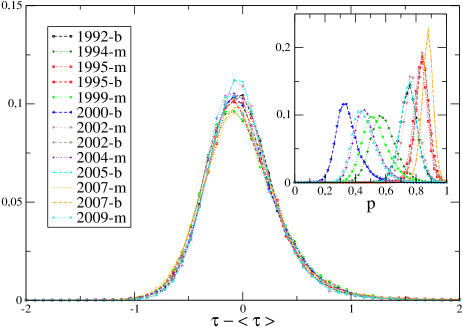
Figure 1: Distribution over communes of $P(\tau-\langle\tau\rangle)$ for each election, where $\tau$ is the logarithmic turnout rate and $\langle\tau\rangle$ its average over all communes. The suffix -b means the election is of binary nature, while -m means multiple choice elections. The inset shows the distributions of direct turnout rates, $p$, for each election.

The issues at stake in all these elections are clearly very different, and so it is not a priori obvious that anything universal (across different elections) can be found in the statistics of votes. However, to our surprise, we found a number of empirical regularities that we now detail, focussing first on turnout rates where these regularities are most robust. Very similar results are also found for winning votes – see below.

The simplest quantity to look at is the pdf of the logarithmic turnout rate $\tau$ over different communes, i.e. what is the probability $P(\tau){\rm d}\tau$ that a given commune, irrespective of its size, has a turnout rate $\tau$ to within ${\rm d}\tau$. Although the average turnout rate $m=\langle\tau\rangle$ varies quite substantially between elections (see Table 1), the shape of the distribution of $\hat{\tau}=\tau-m$ is remarkably constant – even without rescaling by the root mean square $\sigma$, see Fig. 1. The first three cumulants of $P(\tau)$ are, within error bars, the same for all elections (see Table 1). In fact, a Kolmogorov-Smirnov test where one only allows for a relative shift of the distributions does not allow one to reject the hypothesis that $P(\hat{\tau}/\sigma)$ is indeed the same for all elections (except perhaps 2009 which gives marginal results). Note that the distribution of $\tau$ is clearly non Gaussian, with significant positive skewness and kurtosis.

The statistics of $\tau$ does in fact depend on the commune-size $N$. We find that both the mean and variance of the conditional distribution $P(\tau|N)$ decrease with $N$ – see Fig. 2; in particular, small communes have a larger average turnout rate (this explains the positive skewness of $P(\tau)$ noted above Borghesi ), but also a larger dispersion around the average. This is of course expected for a simple binomial process, which predicts that $\sigma_{\tau}^{2}(N)=1/Np(1-p)+\Sigma^{2}$, where $p$ is the ($N$-dependent) average turnout rate, whereas $\Sigma^{2}$ describes the ‘true’ variance of the turnout rate. The simplest assumption is that $\Sigma^{2}$ is $N$-independent, in which case the observed variance varies significantly faster (by a factor $2$ or so) than the simple binomial prediction that assumes independent voters, see Fig. 2, inset. A possible interpretation is that the votes of different individuals are not independent within the same commune, leading to an effectively smaller value of $N$ in the binomial. One can for example assume that within families, or groups of close friends, the decision to vote or not to vote is exactly the same. If the size distribution of these groups of “clones” is $Q(s)$, then it is easy to show that for $N$ large enough, these correlations in decision amount to replacing $N$ by $N\langle s\rangle_{Q}/\langle s^{2}\rangle_{Q}\leq N$. An explicit example is $Q(s)=(1-z)z^{s-1}$ for $s=1,2,\dots$, which leads to an effective value of $N$ reduced by a factor $(1-z)/(1+z)$. In order to account for a factor of $2$ in the variation of $\sigma_{\tau}^{2}$ with $N$, we therefore need to choose $z\approx 1/3$. Since $z$ is the probability that the group is larger than $s=1$, this looks quite large. In fact, as we will discuss below, there is an alternative interpretation of the excess variance that does not rely on direct imitation.

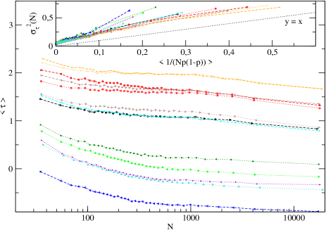
Figure 2: Mean (main figure) and variance (inset) of the conditional distribution $P(\tau|N)$. These quantities are obtained as averages over bins with one thousand communes of size $\approx N$.

Let us now turn to the spatial correlations between turnout rates, measured by the following correlation function:

$$C_{\tau}(r)=\frac{\left.\left\langle(\tau_{\alpha}-m_{\alpha})(\tau_{\beta}-m_{\beta})\right\rangle\right|_{r_{\alpha\beta}=r}}{\langle(\tau_{\alpha}-m_{\alpha})^{2}\rangle},$$ (1)

where $m_{\alpha}$ is the average of $\tau$ over all communes with size in the same “bin” as that of $\alpha$, so as to remove systematic spatial correlations between town sizes. The central result of our empirical study is that for all elections, $C_{\tau}(r)$ is long-range correlated. It is found to decay as the logarithm of the distance (see Fig. 3, left): for $0<r<L$, $C_{\tau}(r)=-\lambda^{2}\ln(r/L)$, and $C_{\tau}(r>L)\approx 0$. Whereas the logarithmic slope $\lambda^{2}$ depends on the election and varies by a factor at most $2$ (between 1999 and 2007) the cut-off distance $L$ is, remarkably similar for all elections, with $L\approx 300$ km. In order to visualise more directly the correlations between neighbouring towns, we have also studied the relation between $\tau_{\alpha}$ and the average of $\tau_{\beta}$ over the 16 $\beta$ towns closest to $\alpha$. We find a very good linear regression between the two over the whole range of $\tau$’s, with a slope equal to unity (not shown, see Borghesi ).

The same general picture holds for the statistics of winning votes, except that: (a) the distribution of the logarithmic winning rate $P(\rho)$ is much less universal across elections than $P(\tau)$. We have noticed in particular that the skewness of $P(\rho)$ varies significantly between elections, and changes sign between presidential elections, where it is positive, and referendums, where it is negative. Contrarily to $\langle\tau\rangle|_{N}$, $\langle\rho\rangle|_{N}$ does not show any systematic pattern, whereas $\sigma_{\rho}^{2}(N)$ is again significantly larger than the simple binomial prediction; (b) the spatial correlation of winning votes $C_{\rho}$ is also logarithmic with $r$ (see Fig. 3, right), although the 2002 result shows a more pronounced curvature. The value of the cut-off distance $L$ is similar to the one reported above, whereas the slope $\lambda^{2}$ tends to be larger, except in the 2000 election (see Borghesi for more details, and also for more statistical regularities in these elections.)

3 Theoretical insights and threshold models

The long-range, logarithmic dependence of the correlation functions $C_{\tau}(r)$ and $C_{\rho}(r)$ is the most striking finding of our study, in particular because it is strongly reminiscent of the behaviour of the correlation function of a free diffusion field in two dimensions. More precisely, let $\phi(\vec{R},t)$ be a two-dimensional field that obeys the following stochastic dynamical equation:

$$\frac{\partial\phi(\vec{R},t)}{\partial t}=D\Delta\phi(\vec{R},t)+\eta(\vec{R},t),$$ (2)

where $\Delta$ is the two-dimensional Laplacian, $D$ is a diffusion constant and $\eta$ a Langevin noise with zero mean, variance $\sigma_{\eta}^{2}$ and short-range correlations both in time and in space. It is well known that the equal-time correlation of $\phi$ is (in equilibrium) given by:

$$C_{\phi}(r)=\frac{\left\langle\phi(\vec{r})\phi(0)\right\rangle}{\langle\phi(0)^{2}\rangle}\approx-\Lambda^{2}{\ln\frac{r}{L}},\qquad\ell_{c}\ll r\ll L,$$ (3)

where $\ell_{c}$ is a short scale cut-off (for example the correlation length of the noise $\eta$) and $L$ is the linear size of the system. The behaviour of $C_{\phi}(r)$ for $r<\ell_{c}$ and the logarithmic slope $\Lambda^{2}$ depend on short scale details of the model, but not on the the diffusion constant $D$. The time to reach equilibrium, beyond which the above result holds, is $T_{eq}=L^{2}/D$. The logarithmic behaviour is a hallmark of the two-dimensional nature of the problem. The striking similarity between this prediction and our empirical findings is the motivation of the theoretical analysis that we present now.

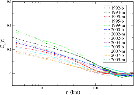
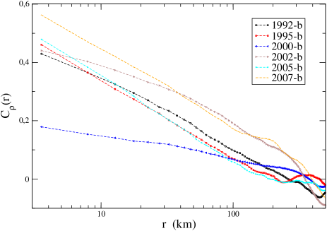
Figure 3: Spatial correlations $C_{\tau}(r)$ of logarithmic turnout rates (left) and $C_{\rho}(r)$ of winning votes (right), showing a logarithmic dependence on $r$ with a cut-off distance $L\approx 300$ km. The average logarithmic slope $\lambda^{2}$ is found to be $\approx 0.065\pm 0.01$ for turnout rates, and $\approx 0.11\pm 0.02$ for winning votes (removing the 2000 referendum on the reform of the presidential mandate, considered to be a very technical subject for which the turnout rate was exceptionally low, see Table 1.)

There is quite a large literature on binary decision models (see granovetter ; Anderson for classical references, and brock ; galam_galam ; collective_shift ; nadal_dicrete_choices ; fortunato_stat_phys ; stauffer_sociophys ; bettencourt_epidemiological ; schweitzer_brownian for more recent contributions), although the spatial correlations that we want to include appear to be new. It is natural to think about these situations in terms of thresholds granovetter : although the decision is binary, the process leading to the final choice is in fact continuous and reflects the individual motivations, propensities or utilities, that we will call the intention $\varphi_{i}$, where $i$ labels the individuals. When $\varphi$ exceeds a certain threshold $\Phi_{c}$, the decision $S$ is one way – say $S=1$; when $\varphi$ is below this threshold, $S=0$. The process $\varphi$ is in general time dependent because individuals are influenced by a variety of factors: what they read, what they hear, what they see contribute to the way they understand a given situation and react to it. Some of these influences are idiosyncratic, i.e. unique to each individual (for example, one may be ill on an election day, meaning that the propensity to go out and vote is very low), while others are common to people living in the same area (for example, the quality of public goods in a given town, or the unemployment rate, etc.). Finally, an important influencing factor is the decision $S_{j}$ made by others, if it is known before making one’s own mind, or by the intentions $\varphi_{j}$ of others (see e.g. granovetter ; galam_galam ; brock ; collective_shift ; nadal_dicrete_choices ; salganik_exp ; collective_attention ). For example, the decision to go see a movie, or to carrying on clapping at the end of concerts or shows, may well depend on what others have done in the past or are currently doing. In the first example, the number of people having already seen the movie feeds back on the motivation of those who have not yet seen it, through box-office charts or word of mouth. In the second example collective_shift , the amplitude of clapping generated by the rest of the crowd can be directly perceived and is an incentive to continue the applause. But in other situations where the decision is taken simultaneously and the final result is only known a posteriori (like in elections), this direct imitation mechanism cannot be present – although of course the influence of intentions is possible, and will be explicitly included in the model below.

The above discussion suggest a general decomposition of the individual intention field $\varphi_{i}$ into an idiosyncratic part, a ‘cultural’ part and an imitation part. More formally, for an individual $i$ living in the vicinity of $\vec{R}$, the intention at time $t$ is written as:

$$\varphi_{i}(t)=\epsilon_{i}(t)+\phi(\vec{R},t)+\sum_{j}J_{ij}S_{j}(t-1);$$ (4)

where $\epsilon_{i}(t)$ is the instantaneous contribution to the intention that is specific to $i$, and $\phi(\vec{R},t)$ is an average of the intentions of the fellow denizens expressed in a recent past. This average can be seen as a space dependent ‘cultural’ field which encodes all the local, stable features that influence the final decision. In essence, this component should be relatively smooth over both space and time. The last term describe the influence of the decision of others, with couplings $J_{ij}$ that measure the strength with which the decision/intention of individual $j$ influences $i$. $J>0$ means conformity of choices, whereas $J<0$ encodes dissent. Many situations (like the movie and the clapping examples given above) are described by a mean-field coupling to the average decision of others: $J_{ij}=J_{0}/N$, $\forall i\neq j$, or to the average intention of others. Finally, the decision rule is $S_{i}(t)=\Theta(\varphi_{i}(t)-\Phi_{c})$, with $\Theta(x\geq 0)=1$ and $\Theta(x<0)=0$. Note that within such a threshold model, the intention field is defined up to an arbitrary scale and shift. There is no physical unit of intention, nor any particular meaning to $\varphi=0$: only differences of intentions can matter in the evolution of the $\varphi_{i}$’s.

Note that without the ‘cultural field’ $\phi(\vec{R},t)$ and with a random static idiosyncratic term $\epsilon_{i}$, Eq. (4) boils down to the Random Field Ising Model galam1 ; sethna_houches , with first applications to social dynamics appearing in galam2 ; galam3 , see also collective_shift ; nadal_dicrete_choices . For early studies and/or critical reflections in sociophysics quetelet , see e.g. ostwald ; majorana ; kadanoff ; batty ; montroll ; toulouse .

As noted above the intra-commune correlations between votes may be due to direct imitations between members of the same family (between which intentions are often shared). But the long-ranged spatial correlations cannot be due to the imitation of decision term. One reason is, as noted above, that elections are not situations where the actual decision of others can matter, since it is known too late. Interestingly, however, the data itself strongly rejects a model where the field $\phi(\vec{R},t)$ is short-ranged correlated, while assigning the spatial correlations of $\tau$ to a coupling term $J_{\alpha\beta}$ between nearby communes. The reason this model cannot be made to work is the following: for long-ranged correlations to emerge, the coupling $J$ must be such that the system is close to its critical point $J_{c}$, beyond which imitation is so strong that the solution of the coupled equations giving the $\{S_{i}\}$ becomes multi-valued. But when this is the case, the corresponding distribution of turnout rates becomes very wide, or even bimodal, and negatively skewed in a way that is incompatible with the unimodal, positively skewed and rather narrow distribution observed empirically (see Fig. 1). A detailed discussion of the inadequacy of this model in the case of elections is provided in Borghesi . The long-ranged correlations of $\tau$ should, we believe, be sought in the spatial structure of the cultural field $\phi(\vec{R},t)$.

From now on, we therefore neglect the direct imitation component in Eq. (4) above. We introduce the cumulative distribution of the instantaneous, idiosyncratic component $\epsilon$: ${\cal P}_{>}(x)=\int_{x}^{\infty}dx^{\prime}P(\epsilon)$. Calling $\pi_{\alpha}={\cal P}_{>}\left(\Phi_{c}-\phi(\vec{R}_{\alpha})\right)$ the theoretical turnout rate of commune $\alpha$, the realized turnout rate is given by:

$$p_{\alpha}=\frac{1}{N_{\alpha}}\sum_{i=1}^{N_{\alpha}}S_{i}\approx\pi_{\alpha}+\sqrt{\frac{\pi_{\alpha}(1-\pi_{\alpha})}{N_{\alpha}}}\xi,\qquad(N_{\alpha}\gg 1)$$ (5)

where $\xi$ a standardised Gaussian noise. We will assume a logistic distribution for $P(\epsilon)$, which will make the following discussion particularly transparent, i.e.:

$${\cal P}_{>}(x)=\frac{1}{1+e^{\frac{x-\mu}{\sigma_{\epsilon}}}},$$ (6)

where $\mu$ is the average of the $\epsilon$ and $\sigma_{\epsilon}$ the width of $P(\epsilon)$ that we assume, for simplicity, to be constant in space and in time, and that we set equal to unity in the following. The average $\mu$ may itself depend both on space and time, and can be seen as an extra, commune specific spatial noise that adds up to the smooth cultural field $\phi$. In fact, we will subtract from $\phi(\vec{R})$ any short-range correlated component that we assign to $\mu(\vec{R})$, such that by definition, the correlation function of the $\phi$ field $C_{\phi}(r)$ tends smoothly towards $1$ when $r\to 0^{+}$.

With this particular logistic choice above, one finds:

$$\tau_{\alpha}=\ln(\frac{p_{\alpha}}{1-p_{\alpha}})$$

$$\approx\left(\phi(\vec{R}_{\alpha})+\mu(\vec{R}_{\alpha})-\Phi_{c}\right)+\frac{1}{\sqrt{\pi_{\alpha}(1-\pi_{\alpha})N_{\alpha}}}\,\xi$$ (7)

Up to a shift and a noise component that vanishes when $N_{\alpha}\to\infty$, $\tau_{\alpha}$ and $\phi(\vec{R}_{\alpha})$ are now the very same object. For other choices of the distribution of $\epsilon$, such a strict identification is not warranted, but we expect that both object share similar statistical properties.

Within the above identification, the variance of $\tau_{\alpha}$ is given by:

$$\sigma^{2}_{\tau}=\sigma^{2}_{\phi}+\sigma^{2}_{\mu}+\langle\frac{1}{Np(1-p)}\rangle\equiv\sigma^{2}_{\phi}\left[1+A\right],$$ (8)

where the ratio of variances $A$ is introduced for later convenience. The variance of the logarithmic turnout rate is therefore the result of three effects: (1) the fluctuations of the smooth cultural field, $\sigma^{2}_{\phi}$. This quantity is not attached to a particular commune and therefore cannot depend on $N$; (2) the fluctuations of the average intentions in a given commune, $\sigma^{2}_{\mu}$, that may well depend on $N$ (a naive guess would be as $N^{-1}$); and (3) the binomial noise effect, that scales as $N^{-1}$. So the extra noise found in the data (see Fig. 2), that we interpreted above as a sign of intra-commune herding, may in fact reveal the contribution of $\sigma^{2}_{\mu}$.

A way to distinguish the two interpretations is to compute the covariance of the $\tau_{\alpha}$ for different elections as a function of $N$, and compare it to the variance of $\tau_{\alpha}$, plotted in Fig. 2. Since the binomial noise is uncorrelated from election to election, its contribution must drop out from the covariance of $\tau$ for different elections, averaged over all communes:

$${\rm{Cov}}_{\tau}(t,t^{\prime})=\langle\tau_{\alpha}(t)\tau_{\alpha}(t^{\prime})\rangle_{c}$$

$$=\langle\phi_{\alpha}(t)\phi_{\alpha}(t^{\prime})\rangle_{c}+\langle\mu_{\alpha}(t)\mu_{\alpha}(t^{\prime})\rangle_{c},\quad(t\neq t^{\prime}),$$ (9)

where the index ‘c’ means that we take a cumulant average over all pairs of elections and all communes. If the binomial noise was the only source of the $N$ dependence of $\sigma^{2}_{\tau}$, the above covariance of the $\tau$s at different times should be independent of $N$. This is not what the data shows. There is indeed a residual $N$-dependence that must be ascribed to the statistics of the average of idiosyncratic intentions, $\mu(\vec{R})$ (although we have no interpretation for the $\sim N^{-3/2}$ dependence that we observe. The assumption that the dispersion of individual biases, $\sigma_{\epsilon}$, is commune-independent might in fact not be warranted). Interestingly, we have found that the following relation accounts very well for the data:

$$\langle{\rm{Cov}}_{\tau}(t,t)\rangle_{t}\approx B\langle{\rm{Cov}}_{\tau}(t,t^{\prime})\rangle_{t\neq t^{\prime}}+\left\langle\frac{1}{Np(1-p)}\right\rangle,$$ (10)

where $B\approx 1.5$. The remarkable point of this analysis is that the coefficient of the binomial contribution is found to be exactly unity, meaning that within this interpretation one does not need to invoke the presence of intra-communes “clones”, or more precisely that the probability $z$ of herds is too small to be detectable using our data set The coefficient $B$ simply accounts for the average decay of the correlation of $\phi$ and $\mu$ as a function of time, and its value is compatible with the results shown in Fig. 5 below.

4 The random diffusion equation

We will now argue why it is natural to expect that the cultural field $\phi(\vec{R}_{\alpha},t)$ should obey a noisy diffusion equation akin to Eq. (2) with an extra global, time dependent driving term. Although $\phi(\vec{R}_{\alpha},t)$ is an rather abstract object, the existence of which we postulate, its time evolution should contain a random term that describes events that are specific both in time and in space and contribute to changing the overall mood of a given city, such as the closing down of a factory or of a military base, important changes in population, or a particularly charismatic local leader, for example. This is captured by the term $\eta(\vec{R},t)$, which we imagine to be correlated in space over some length scale $\ell_{c}$ comparable to the typical inter-commune distance, and over a time $T_{c}$ of, plausibly, several months.

The Laplacian term describes the fact that people themselves move around and carry with them some components of the local cultural specificity $\phi(\vec{R}_{\alpha},t)$. This can be either by actually moving to a nearby city, or by just visiting or interacting with acquaintances from the neighbouring cities. The all year round exchange of ideas, informations and experiences must lead to a local propagation of $\phi(\vec{R}_{\alpha},t)$. Since only difference of intentions matter, the evolution of the cultural field at $\vec{R}_{\alpha}$ can only depend on the differences $\phi(\vec{R}_{\beta},t)-\phi(\vec{R}_{\alpha},t)$; furthermore, the model must be invariant under a change of scale of $\phi$. In order to satisfy these constraints, the most general term describing the evolution of $\phi(\vec{R}_{\alpha},t)$ due to the surrounding influences takes the following, linear form:

$$\left.\frac{\partial\phi(\vec{R}_{\alpha},t)}{\partial t}\right|_{\rm{infl.}}=\sum_{\beta}\Gamma_{\alpha\beta}[\phi(\vec{R}_{\beta},t)-\phi(\vec{R}_{\alpha},t)],$$ (11)

where $\Gamma_{\alpha\beta}(r_{\alpha\beta})\geq 0$ is a symmetric influence matrix, that we assume to decrease over a distance corresponding to typical daily displacements of individuals, say $10$ km or so. The above equation means that through human interactions, the cultural differences between nearby cities tend to narrow. As is well known, the continuum limit of the right hand side of Eq. (11) reads $\vec{\nabla}\cdot[D(\vec{R})\vec{\nabla}\phi(\vec{R},t)]$, with $D(\vec{R}_{\alpha})=\frac{1}{2}\sum_{\beta}r_{\alpha\beta}^{2}\Gamma_{\alpha\beta}$ is a (space dependent) measure of the speed at which the cultural field diffuses. This spatial dependence is a priori expected: for example, $D(\vec{R})$ should presumably be smaller in mountain regions (because of the difficulty to travel from one valley to the next) or in sparsely populated areas (because of the larger distance between neighbouring towns).

Our final equation, that respects all the symmetries of the model , is therefore (in the continuum limit):

$$\frac{\partial\phi(\vec{R},t)}{\partial t}=\vec{\nabla}\cdot[D(\vec{R})\vec{\nabla}\phi(\vec{R},t)]+\eta(\vec{R},t)+\nu(\vec{R})F(t),$$ (12)

where $F(t)$ represents the public information, for example the subject and importance of the election, national TV programs, etc. In principle, different communes may react differently to the same public information, leading to space dependent ‘reactivity’ $\nu(\vec{R})$, but we will neglect these spatial fluctuations in the following. Similarly, we assume that the variance and higher cumulants of $\eta$ are homogeneous and independent of the size of the commune, but this assumption could be relaxed if needed. Because any average trend is described by $F(t)$, the noise $\eta(\vec{R},t)$ is of zero mean. The average trend can be accounted for by a uniform shift of $\phi$:

$$\phi(\vec{R},t)\longrightarrow\phi(\vec{R},t)-\nu\int_{0}^{t}{\rm d}t^{\prime}F(t^{\prime}).$$ (13)

This explains why the average value of $\phi$, and therefore of the turnout rate $\tau$, can change substantially over time, while the fluctuations of $\phi$ and its spatial correlations remain essentially stable – as found empirically, see Figs. 1 and 3.

When $D(\vec{R})=D$ is uniform, we recover Eq. (2) and the logarithmic decay of the correlation function $C_{\tau}(r)\propto C_{\phi}(r)$ follows immediately, since the contribution of the idiosyncratic $\mu$ field and the binomial noise, both short ranged in space, rapidly disappear when $r>0$. Since we have removed from $\phi$ its short range spatial contribution, the coefficient $\Lambda^{2}$ appearing in Eq. (3) is given by $1/\ln\frac{L}{\ell_{c}}$. Therefore,

$$C_{\tau}(r\neq 0)=\frac{C_{\phi}(r)}{1+A}\approx\frac{1}{1+A}\times\frac{\ln\frac{L}{r}}{\ln\frac{L}{\ell_{c}}},$$ (14)

where $A$ is the ratio of the variance of the idiosyncratic and binomial noise to that of the cultural field, defined in Eq. (8) above. From Fig. 3, one sees that $1/(1+A)\sim 0.2-0.4$ for turnout rates: the cultural field explains roughly a third of the variance of the local results. This ratio increases to one half for winning votes, except for the 2000 referendum (see Fig. 3, right plot), meaning that the role of the cultural field is arguably stronger for polarized political decisions than it is for the question of participating or not to a vote.

When $D(\vec{R})$ is non uniform, the equilibrium correlation of $\phi(\vec{R})$ cannot be computed in general. However, drawing analogies from physics physrep , we know that this inhomogeneous diffusion equation can be, under rather general hypothesis on the statistics of $D(\vec{R})$, “homogeneized”. This means that coarse graining on sufficiently large scales, larger than the correlation length of $D(\vec{R})$, the effective equation becomes identical to Eq. (2) with an effective diffusion constant $\overline{D}$ that can be computed using e.g. perturbation theory, or effective medium approximations physrep . What is of interest for our discussion is that the logarithmic dependence of $C_{\phi}(r)$, Eq. (3), is still valid on large enough scales.

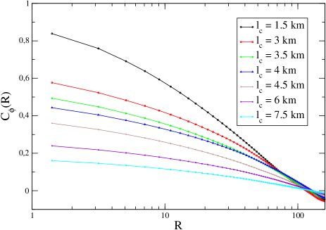
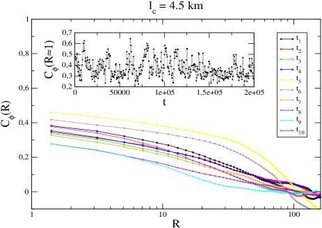
Figure 4: Numerical simulation of the diffusive field model, with the true positions of the French communes, and an interaction between nearby communes decaying as $\exp(-r/\ell_{c})$. Left, we show the correlation $C_{\phi}(R)$ as a function of $\ell_{c}$, after transient regime and averaged over many realizations of the ‘noise’ $\eta$. The distance $R$ is here measured in units of the average inter-commune distance (that depends on the departement. $R=100$ corresponds to $270$ km, precisely the scale at which the empircal correlations reach zero. Right, ten realizations of $C_{\phi}(R)$ for $\ell_{c}=4.5$ km, still after transient regime, as a function of the scaled distance $R$. In the inset, value of the nearest neighbour correlation $C(R=1)$ as a function of ‘time’, showing strong fluctuations.

In order to test these ideas more quantitatively, we have simulated the model using Eq. (11) with the exact locations of all french communes, and $\Gamma_{\alpha\beta}(r)=e^{-r/\ell_{c}}$. The spatially inhomogeneities are therefore treated exactly. We show the resulting spatial correlations of $\phi(\vec{R})$ in Fig. 4-left, for different values of $\ell_{c}$, in the range $[1.5,7.5]$ km, i.e. comparable with the inter-town average distance. We see that $C_{\phi}(r)$ is indeed approximately logarithmic and looks actually very similar to the empirical curves. Note in particular that while the small $r$ value of $C_{\phi}(r)$ and the logarithmic slope $\Lambda^{2}$ significantly depends on $\ell_{c}$, as expected, the point $r$ at which $C_{\phi}(r)$ reaches zero is approximately constant, and, remarkably, very close to its empirical counterpart ($L\approx 300$ km, on the order of the size of the system). It is tempting to associate the apparent dependence of $\lambda^{2}$ on the election to a temporal evolution of $\ell_{c}$. However, this is not correct: our numerical simulations show that even when the system is equilibrated (i.e. when $t\gg L^{2}/D$), the measured $C_{\phi}(r)$ for a fixed value of $\ell_{c}$ fluctuates quite strongly between different realizations of the noise $\eta$, see Fig. 4-right. The range over which $\Lambda^{2}$ varies in the simulation is very similar to what is found empirically. Therefore, the empirical results are fully compatible with a fixed value of $\ell_{c}$. Matching the average empirical slope to the numerical data and taking into account the value of $A$ suggests that $\ell_{c}$ must be very small, of the order of a few kms, fully compatible with our interpretation. We have checked in our numerical simulations that our diffusive field model indeed reproduces the strong linear correlation between $\tau_{\alpha}$ and the average value of $\tau_{\beta}$ over the neighbouring towns, with unit slope. This is of course expected and is the essence of the model, since the Laplacian coupling in Eq. (2) says precisely that on average the Laplacian of $\phi$ is zero, i.e. that $\phi_{\alpha}$ is on average equal to $\sum_{\beta\in n(\alpha)}\phi_{\beta}$, where $n(\alpha)$ is the neighbourhood of $\alpha$. This empirical finding can in fact be seen as a direct, microscopic motivation for postulating Eq. (11) above.

In order to estimate the diffusion of intentions $D$, one can assume that a substantial fraction of the population of a given town experiences some interaction with neighbouring towns after several weeks. For opinions to get closer, this time is probably more on the scale of months. Taking the relevant inter-town distance to be $\sim 10$ km leads to a diffusion constant of the order of $D\sim 100$ km²/month or less (ways of obtaining more precise empirical estimates of this quantity would be important here). The corresponding equilibration time $T_{eq}$ over $L=300$ km is therefore quite long, a century or more. But this is compatible with the fact that the voting habits of the different regions seem to be extremely persistent in history – which is in itself a strong argument for the existence of a cultural field that keeps the memory independently of the presence of particular individuals. This justifies the apparent correlation between geography and votes discussed long ago by Siegfried Siegfried (Le granite vote à droite, le calcaire vote à gauche). Interestingly, a more precise prediction of our model is that the temporal autocorrelation of $\phi$ for a given $\vec{R}$ should behave as:

$$C_{\phi}(t)=\frac{\left\langle\phi(\vec{R},t)\phi(\vec{R},0)\right\rangle}{\langle\phi(\vec{R},t)^{2}\rangle} \approx-\frac{\Lambda^{2}}{2}{\ln\frac{t}{T_{eq}}},$$ (15)

$$\frac{\ell_{c}^{2}}{D},T_{c}\ll t\ll T_{eq},$$

where the slope is exactly one half of the slope of $C_{\phi}(r)$ versus $-\ln r$, and $T_{c}$ the correlation time of the noise $\eta$. We have tested this prediction directly on data, by studying the autocorrelation of the fluctuations of the participation rate for a given commune across different elections, averaged over all communes. Although the data is noisy, see Fig. 5, the results are indeed compatible with a logarithmic decay in time with a slope that has the correct order of magnitude. From the spatial correlations of $\tau$ we find $\lambda^{2}\approx 0.065$ (averaged over all elections – see Fig. 3), whereas the linear regression of $C_{\tau}(t)$ as a function of $\ln t$ gives as slope of $\approx-0.066$. The discrepancy with the factor 2 predicted by the theory could be related to the fact that the autocorrelation in time is substantially larger than the correlation in space (compare Figs. 3 and 5), meaning that the idiosyncratic field $\mu(\vec{R},t)$ has substantially longer temporal correlations than spatial correlations. If the correlation time of the noise $\eta$ is of several months, the contribution of the decorrelation of $\mu(\vec{R},t)$ to $C_{\tau}(t)$ probably interferes with the contribution of the cultural field $\phi$ and effectively increases the empirical slope. In any case, in the absence of more information on the dynamics of the $\mu$ field, we find the overall agreement between the model and the behaviour of these temporal autocorrelations satisfying.

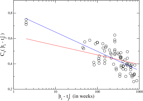
Figure 5: Temporal correlation $C_{\tau}(t)$ of turnout rates $\tau$. Here, $t=|t_{i}-t_{j}|$ where $t_{i}$ and $t_{j}$ are the election dates of elections. The red line shows the expected $C_{\tau}(t)\sim-\frac{1}{2}\lambda^{2}\ln(t)$ where $\lambda^{2}\approx 0.065$ is the averaged slope over all elections of the spatial correlations $C_{\tau}(r)\sim-\lambda^{2}\ln(r)$. The blue line shows the linear regression of $C_{\tau}(t)$ as a function of $\ln(t)$, here with a slope of $\approx-0.066$.

5 Conclusion

Let us summarise the main messages of this study. First, the statistics of the turnout rates in French elections is found to be surprisingly stable over time, once the average turnout rate is factored in. The size dependence of the turnout rate variance may have suggested some intra city ‘herding’ effect, but we believe that the data is more consistent with small towns having a larger dispersion in local, idiosyncratic biases. A convincing argument for why this should be so is however lacking. An explanation could be the systematic difference in the socio-cultural background of the population of large cities compared to that of small cities.

Second, for our whole set of elections, the spatial correlation of the turnout rates, or of the fraction of winning votes, is found to decay logarithmically with the distance between towns. This slow decay of the correlations is characteristic of a diffusive random field in two dimensions. This result is robust against many non essential modifications of the basic version of the model, much as the statistics of a random walk is robust against modifications of the microscopic construction rules. Based on these empirical observations and on the analogy with the two-dimensional random diffusion equation, we have proposed that individual decisions can be rationalised in terms of an underlying “cultural” field that locally biases the decision of the population of a given region, on top of an idiosyncratic, city-dependent field, with short range correlations.

Based on symmetry considerations and a set of plausible arguments, we have suggested that this cultural field obeys an equation in the universality class of the random diffusion equation, Eq. (12) above. We believe that similar considerations should hold for other decision processes, such as consumption habits, behavioral biases, etc. More empirical work on the spatial correlations of these decisions, in different situations and in different countries, would be very valuable to test our claim of universality. Direct estimates of the parameters of the model, such as the value of the diffusion constant $D$ or the relative strength of the idiosyncratic field, are clearly needed at this stage. We hope that our work will motivate more empirical studies to refine and calibrate the model proposed here.

References

- (1) M. Granovetter, Threshold models of collective behaviour, Am. J. Sociol. 83, 1420 (1978); M. Granovetter, R. Soong, Threshold models of diffusion and collective behaviour, J. Math. Socio. 9, 165 (1983).
- (2) T. Schelling, Micromotives & Macrobehaviour New York, Norton (1978).
- (3) E. M. Rogers, Diffusion of innovations, (4th ed.), Free Press, New York (1995).
- (4) S. Galam, Sociophysics: A review of Galam models, Int. J. Mod. Phys. C 19, 409-440 (2008).
- (5) W. Brock, S. Durlauf, Discrete choices with social interactions, Rev. Economic Studies, 68, 235 (2001).
- (6) see e.g. D. Helbing, I. J. Farkas, and T. Vicsek, Crowd disasters and simulation of panic situations, in: A. Bunde, J. Kropp, and H.-J. Schellnhuber (eds.) The Science of Disasters. Climate Disruptions, Heart Attacks, and Market Crashes, p 334, Springer, Berlin (2002).
- (7) Q. Michard and J.-P. Bouchaud, Theory of collective opinion shifts: from smooth trends to abrupt swings, Eur. Phys. J. B 47, 151-159 (2005).
- (8) M. B. Gordon, J.-P. Nadal, D. Phan and V. Semeshenko, Discrete Choices under Social Influence: Generic Properties, Math. Models and Methods in Applied Sciences (M3AS), 19, Sup. Issue 1, 1441-1481 (2009).
- (9) M. J. Salganik, P. S. Dodds, D. J. Watts, Experimental Study of Inequality and Unpredictability in an Artificial Cultural Market, Science 311, 854-856 (2006).
- (10) C. Borghesi and J.-P. Bouchaud, Of Songs and Men: a Model for Multiple Choice with Herding, Qual. Quant. 41, 557-568 (2007).
- (11) A. Siegfried, Tableau politique de la France de l’ouest sous la troisième république, Ed. A. Colin (1913).
- (12) Michel Bussi, Éléments de géographie électorale à travers l’exemple de la France de l’Ouest, Ed. P. U. de Rouen (1998).
- (13) N. Ganache, Le mythe du paysage qui vote, http://norois.revues.org/index594.html (2005).
- (14) R. N. Costa Filho, M. P. Almeida, J. S. Andrade Jr., and J. E. Moreira, Scaling behavior in a proportional voting process, Phys. Rev. E 60, 1067-1068 (1999).
- (15) R. N. Costa Filho, M. P. Almeida, J. E. Moreira and J. S. Andrade Jr., Brazilian elections: voting for a scaling democracy, Phys. A 322, 698-700 (2003).
- (16) M. L. Lyra, U. M. S. Costa, R. N. Costa Filho and J. S. Andrade, Generalized Zipf’s law in proportional voting processes, Europhys. Lett. 62, 131-137 (2003).
- (17) A. T. Bernardes, D. Stauffer and J. Kertész, Election results and the Sznajd model on Barabasi network, Eur. Phys. J. B 25, 123-127 (2002).
- (18) M.C. Gonzalez, A.O. Sousa and H.J. Herrmann, Opinion Formation on a Deterministic Pseudo-fractal Network, Int. J. Mod. Phys. C 15(1), 45-47 (2004).
- (19) S. Sinha and R. K. Pan, How a “Hit” is born: The Emergence of Popularity from the Dynamics of Collective Choice, in Econophysics and Sociophysics: Trends and Perspectives, Ed. Wiley, 2006 ; arXiv:0704.2955 [physics.soc-ph].
- (20) G. Báez, H. Hernández-Saldaña and R.A. Méndez-Sánchez, Statistical properties of electoral systems: the Mexican case, arXiv: physics/0609114.
- (21) O. Morales-Matamoros, M. A. Martínez-Cruz and R. Tejeida-Padilla, Mexican Voter Network as a Dynamic Complex System, in 50th Annual Meeting of the ISSS (2006).
- (22) H. Situngkir, Power-Law Signature in Indonesian Legislative Election 1999 and 2004, arXiv: nlin/0405002.
- (23) S. Fortunato and C. Castellano, Scaling and universality in proportional elections, Phys. Rev. Lett. 99, 138701 (2007).
- (24) L. E. Araripe, R. N. Costa Filho, H. J. Herrmann, and J. S. Andrade Jr., Plurality Voting: the statistical laws of democracy in Brazil, Int. J. Mod. Phys. C 17, 1809 (2006).
- (25) M. G. Sadovsky, A. A. Gliskov, Towards the Typology of Elections at Russia, arXiv:0706.3521 [physics.soc-ph].
- (26) J. J. Schneider and Ch. Hirtreiter, The Impact of Election Results on the Member Numbers of the Large Parties in Bavaria and Germany, Int. J. Mod. Phys. C 16, 1165-1215 (2005).
- (27) H. Hernández-Saldaña, On the Corporate Votes and their relation with Daisy Models, arXiv:0810.0554 [physics.soc-ph].
- (28) Chung-I Chou and Sai-Ping Li, Growth Model for Vote Distributions in Elections, arXiv:0911.1404 [physics.soc-ph].
- (29) D. M. Romero, C. M. Kribs-Zaleta, A. Mubayi and C. Orbe, An Epidemiological Approach to the Spread of Political Third Parties, arXiv:0911.2388 [physics.soc-ph].
- (30) S. Banisch and T. Araùjo, On the Empirical Relevance of the Transient in Opinion Models, arXiv:1003.5578 [physics.soc-ph].
- (31) A. Blais, To vote or not to vote? The Merits and Limits of Rational Choice Theory, Univerity of Pittsburg Press (2000).
- (32) M. Franklin, Voter Turnout and the Dynamics of Electoral Competition in Established Democracies since 1945, Cambridge U. P. (2004).
-
(33)
French Home Office, bureau des élections et des études politiques, http://www.
interieur.gouv.fr/sections/a_votre_service/elections/resultats -
(34)
Institut Géographique National
http://professionnels.ign.fr/ficheProduitCMS.do?idDoc=5323862 - (35) C. Borghesi, Une étude de physique sur les élections – Régularités, prédictions et modèles sur des élections françaises, PhD Thesis, arXiv:0910.4661 [physics.soc-ph].
- (36) S. P. Anderson, A. De Palma, J. F. Thisse, Discrete choice theory of product differentiation, Cambridge, MIT press (1992).
- (37) C. Castellano, S. Fortunato and V. Loreto, Statistical physics of social dynamics, Rev. Mod. Phys. 81, 591-646 (2009).
- (38) D. Stauffer, Opinion Dynamics and Sociophysics, in Encyclopedia of Complexity and Systems Science, p. 6380-6388, Ed. Springer, 2009 ; arXiv:0705.0891 [physics.soc-ph].
- (39) L. M. A. Bettencourt, A. Cintrón-Arias, D. I. Kaiser and C. Castillo-Chávez, The power of a good idea: Quantitative modeling of the spread of ideas from epidemiological models, Physica A, 364, 513-536 (2006).
- (40) F. Schweitzer, Brownian Agents and Active Particles: Collective Dynamics in the Natural and Social Sciences, Ed. Springer (2003).
- (41) M. J. Hinish, M. C. Munger, Ideology and the Theory of Political Choice, University of Michigan Press (1994).
- (42) M. Moussaid, D. Helbing and G. Theraulaz, An individual-based model of collective attention, arXiv:0909.2757 [physics.soc-ph].
- (43) F. Caccioli, S. Franz and M. Marsili, Ising model with memory: coarsening and persistence properties, J. Stat. Mech. P07006 (2008).
- (44) S. Galam, A new multicritical point in anisotropic magnets. III. Ferromagnets in both a random and a uniform longitudinal field, J. Phys. C: Solid State 15, 529 (1982).
- (45) J. P. Sethna, Crackling Noise and Avalanches: Scaling, Critical Phenomena, and the Renormalization Group, in Complex Systems, Volume LXXXV: Lecture Notes of the Les Houches Summer School 2006, 257-288, Ed. Elsevier, 2007 (arXiv: cond-mat/0612418).
- (46) S. Galam and S. Moscovici, Towards a theory of collective phenomena: Consensus and attitude changes in groups, Eur. J. Soc. Psy. 21, 49- (1991).
- (47) S. Galam, Rational group decision making : a random field Ising model at T = 0 , Physica A, 238, 66 (1997).
- (48) A. Quetelet, Physique sociale, ou Essai sur le développement des facultés de l’homme, Muquardt, Brussels (1835, 1869).
- (49) W. Ostwald, Energetische grundlagen der kulturwissenschaften, W. Klinkhardt, Leipzig (1909).
- (50) E. Majorana, Il valore delle Leggi statistiche nella fisica e nelle scienze sociali, Scientia, 36, 58–66 (1942) ; arXiv:0709.3537 [physics.soc-ph].
- (51) L. P. Kadanoff, From simulation model to public policy: An examination of Forrester’s ‘Urban Dynamics’, Simulation 16, 261-268 (1971).
- (52) M. Batty, Urban modelling: Algorithms, calibrations, predictions, Cambridge U. P. (1976).
- (53) E. W. Montroll, Social dynamics and the quantifying of social forces, Proc. Natl. Acad. Sci. USA, 75, No. 10, 4633-4637 (1978).
- (54) G. Toulouse and J. Bok, Principe de moindre difficulté et structures hiérarchiques, Rev. franç. socio. 19, 391-406 (1978).
- (55) see e.g.: J.P. Bouchaud, A. Georges, Anomalous diffusion in disordered media, Phys. Rep. 195 127-293 (1990).