An overview of latent Markov models for longitudinal categorical data

Abstract

We provide a comprehensive overview of latent Markov (LM) models for the analysis of longitudinal categorical data. The main assumption behind these models is that the response variables are conditionally independent given a latent process which follows a first-order Markov chain. We first illustrate the basic LM model in which the conditional distribution of each response variable given the corresponding latent variable and the initial and transition probabilities of the latent process are unconstrained. For this model we also illustrate in detail maximum likelihood estimation through the Expectation-Maximization algorithm, which may be efficiently implemented by recursions known in the hidden Markov literature. We then illustrate several constrained versions of the basic LM model, which make the model more parsimonious and allow us to include and test hypotheses of interest. These constraints may be put on the conditional distribution of the response variables given the latent process (measurement model) or on the distribution of the latent process (latent model). We also deal with extensions of LM model for the inclusion of individual covariates and to multilevel data. Covariates may affect the measurement or the latent model; we discuss the implications of these two different approaches according to the context of application. Finally, we outline methods for obtaining standard errors for the parameter estimates, for selecting the number of states and for path prediction. Models and related inference are illustrated by the description of relevant socio-economic applications available in the literature.

math.PR/0000000

and

1 Introduction

In many applications involving longitudinal data, the interest is often focused on the evolution of a latent characteristic of a group of individuals over time, which is measured by one or more occasion-specific response variables. This characteristic may correspond, for instance, to the quality-of-life of subjects suffering from a certain disease, which is indirectly assessed on the basis of responses to a set of suitably designed items that are repeatedly administered during a certain period of time.

In the statistical and econometric literatures, several approaches have been introduced to address the above issue. Among these approaches, one of the most interesting is based on the same formulation of the hidden Markov model for time series (Baum and Petrie,, 1966; MacDonald and Zucchini,, 1997). The main assumption behind this approach is that the response variables are conditionally independent given a latent Markov chain with a finite number of states. The basic idea behind this assumption, that we will refer to as the assumption of local independence, is that the latent process fully explains the observable behavior of a subject; moreover, the latent state to which a subject belongs at a certain occasion only depends on the latent state at the previous occasion.

The starting point of the paper is the latent Markov (LM) model. This model dates back to Wiggins’ Ph.D. thesis, Wiggins, (1955), who introduced a version of this model based on a homogenous Markov chain, a single outcome at each occasion, and did not account for individual covariates. Wiggins, (1955) formulated the model so that a manifest transition is a mixture of a true change and a spurious change due to measurement errors in the observed states. See also Wiggins, (1973) for a deep illustration of this model and some simple generalizations. It is also worth mentioning Van de Pol and De Leeuw, (1986), van de Pol and Langeheine, (1990), Collins and Wugalter, (1992), and Langeheine and Van de Pol, (1994), among the first papers dealing with this model.

In the following, we refer to the LM model based on a first-order Markov chain, non-homogeneous transition probabilities, and no covariates as the basic LM model. This model may be used for univariate or multivariate data; in the second case we observe more response variables at each occasion. For the basic LM model we discuss in detail maximum likelihood estimation through the Expectation-Maximization (EM) algorithm (Baum et al.,, 1970; Dempster et al.,, 1977), even though we acknowledge that other estimation methods are available (Archer and Titterington,, 2009; Cappé et al.,, 1989; Künsch,, 2005; Turner,, 2008). For the implementation of the EM algorithm we illustrate suitable recursions which allow us to strongly reduce the computational effort.

The paper also focuses on several constrained versions and extensions of the basic LM model. Constraints have the aim of making the model more parsimonious and easier to interpret and correspond to certain hypotheses that may be interesting to test. These constraints may be posed on the measurement model, i.e. the conditional distribution of the response variables given the latent process, or on the latent model, i.e. the distribution of the latent process. About the measurement model, we discuss in detail Rasch, (1961) type parameterizations which make the latent states interpretable in terms of ability or propensity levels. About the latent model, we outline several simplifications of the transition matrix, mostly based on constraints of equality between certain elements of this matrix and/or on the constraint that some elements are equal to 0. One of the main problems is how to test for these restrictions. For this aim, we make use of the likelihood ratio (LR) statistic. It is important to note that, when constrains concern the transition matrix, the null asymptotic distribution does not necessarily have an asymptotic chi-squared distribution, but a distribution of chi-bar-squared type (Bartolucci,, 2006).

The most natural extension of the basic LM model is for the inclusion of individual covariates. In particular, we describe two different ways of including such covariates: (i) in the measurement model, so that they affect the conditional distribution of the response variables given the latent process (Bartolucci and Farcomeni,, 2009); (ii) in the latent model, so that they affect the initial and the transition probabilities of the Markov chain (Vermunt et al.,, 1999; Bartolucci et al., 2007b, ). Further, we discuss methods to relax the assumption of local independence and show multilevel LM models which are suitable when subjects are collected in clusters. In this context, the model may be formulated by including fixed parameters to represent the effect of the clusters on the distribution of the latent process corresponding to every subject belonging to these clusters; this approach was followed by Bartolucci et al., (2009). Otherwise, the model may be formulated by including random parameters having a discrete distribution, following in this way an approach similar to that behind the latent class model, as in Bartolucci et al., (2010). This extension is related to the mixed LM model (van de Pol and Langeheine,, 1990) and to the LM model with random effects (Altman,, 2007).

Finally, we revise methods for obtaining standard errors for the model parameters and for selecting the number of latent states. We also discuss the problem of path prediction through the Viterbi algorithm (Viterbi,, 1967; Juang and Rabiner,, 1991).

An important point to clarify is that, throughout the paper, we consider the case of categorical response variables because this is the typical case of application of the LM model. However, it is straightforward to modify the framework to deal with continuous outcomes. Most of the theory and estimation methods do not change substantially.

The paper is organized as follows. In the Section 2 we outline the basic LM model and discuss maximum likelihood estimation for this model based on the EM algorithm. In Section 3 we outline constrained versions of the LM model based on parsimonious and interpretable parameterizations. In Section 4 we illustrate how to deal with individual covariates, whereas the multilevel extension is presented in Section 5. Section 6 deals with standard errors, selection of the number of states, and path prediction. Section 7 illustrates different types of LM model through various examples involving longitudinal categorical data, summarizing the results from other papers. The paper ends with a section where we draw main conclusions and discuss further developments of the present framework.

2 Basic latent Markov model and its multivariate version

In the following, we illustrate the basic LM model for univariate categorical data without covariates and in which the latent Markov chain is of first-order and non-homogenous. We also describe the EM algorithm for maximum likelihood estimation of this model.

2.1 Basic formulation of univariate responses

Let $\mbox{\boldmath$Y$}_{i}=(Y^{(1)}_{i},\ldots,Y_{i}^{(T)})$, $i=1,\ldots,n$, be a sequence of $T$ categorical response variables with $l$ levels or categories, coded from $0$ to $l-1$, independently observed over $n$ subjects. Typically, these variables have the same nature, as they correspond to repeated measurements on the same subjects at different occasions. However, the approach may be applied to the case of response variables having a different nature and, possibly, a different number of categories.

The main assumption of the basic LM model is that of local independence, i.e. for every subject $i$ the response variables in $\mbox{\boldmath$Y$}_{i}$ are conditionally independent given a latent process $\mbox{\boldmath$U$}_{i}=(U^{(1)}_{i},\ldots,U^{(T)}_{i})$. This latent process is assumed to follow a first-order Markov chain with state space $\{1,\ldots,k\}$. Then, for all $t>2$, the latent variable $U^{(t)}_{i}$ is conditionally independent of $U^{(1)}_{i},\ldots,U^{(t-2)}_{i}$ given $U^{(t-1)}_{i}$. See Figure 1 for an illustration via path diagram.

Figure 1: Path diagram of the basic LM model for univariate data.

The latent process can be used to model a real unidimensional latent trait evolving over time, or just as a parsimonious device to allow for a time non-homogeneous distribution for the sequence $\mbox{\boldmath$Y$}_{i}$. The Markov assumption is seldom found to be restrictive, and is easily interpretable. A further interpretation of the model is given by the measurement error framework: the unobservable outcome $U^{(t)}_{i}$ is observed with measurement error as $Y^{(t)}_{i}$. Therefore, it may be seen as an extension of a standard Markov model (Anderson,, 1954); for a discussion on this point see (Wiggins,, 1973, Chapter 4).

Parameters of the model are the conditional response probabilities $\phi_{y|u}^{(t)}=p(Y^{(t)}_{i}=y|U^{(t)}_{i}=u)$, $t=1,\ldots,T$, $u=1,\ldots,k$, $y=0,\ldots,l-1$, the initial probabilities $\pi_{u}=p(U^{(1)}_{i}=u)$, $u=1,\ldots,k$, and the transition probabilities $\pi_{v|u}^{(t)}=p(U^{(t)}_{i}=v|U^{(t-1)}_{i}=u)$, $t=2,\ldots,T$, $u,v=1,\ldots,k$. Note that all these probabilities do not depend on $i$ since, in its basic version, the model does not account for individual covariates.

On the basis of the above parameters, the distribution of $\mbox{\boldmath$U$}_{i}$ may be expressed as

$$p(\mbox{\boldmath$U$}_{i}=\mbox{\boldmath$u$})=\pi_{u^{(1)}}\prod_{t>1}\pi_{u^{(t)}|u^{(t-1)}}^{(t)},$$ (1)

where $\mbox{\boldmath$u$}=(u^{(1)},\ldots,u^{(T)})$. Moreover, the conditional distribution of $\mbox{\boldmath$Y$}_{i}$ given $\mbox{\boldmath$U$}_{i}$ may be expressed as

$$p(\mbox{\boldmath$Y$}_{i}=\mbox{\boldmath$y$}|\mbox{\boldmath$U$}_{i}=\mbox{\boldmath$u$})=\prod_{t}\phi_{y^{(t)}|u^{(t)}}^{(t)},$$

and, consequently, for the manifest distribution of $\mbox{\boldmath$Y$}_{i}$ we have

$$\hskip 21.33955ptf(\mbox{\boldmath$y$}) = p(\mbox{\boldmath$Y$}_{i}=\mbox{\boldmath$y$})=\sum_{\mbox{\footnotesize\boldmath{$u$}}}f(\mbox{\boldmath$u$},\mbox{\boldmath$y$})=$$

$$= \sum_{u^{(1)}}\phi_{y^{(1)}|u^{(1)}}^{(1)}\pi_{u^{(1)}}\sum_{u^{(2)}}\phi_{y^{(2)}|u^{(2)}}^{(2)}\pi_{u^{(2)}|u^{(2)}}^{(2)}\cdots\sum_{u^{(T)}}\phi_{y^{(T)}|u^{(T)}}^{(T)}\pi_{u^{(T)}|u^{(T-1)}}^{(T)},$$

where $\mbox{\boldmath$y$}=(y^{(1)},\ldots,y^{(T)})$ and $f(\mbox{\boldmath$u$},\mbox{\boldmath$y$})=p(\mbox{\boldmath$Y$}_{i}=\mbox{\boldmath$y$}|\mbox{\boldmath$U$}_{i}=\mbox{\boldmath$u$})p(\mbox{\boldmath$U$}_{i}=\mbox{\boldmath$u$})$. It is important to note that computing $f(\mbox{\boldmath$y$})$ as expressed above involves a sum extended to all the possible $k^{T}$ configurations of the vector $u$; this typically requires a considerable computational effort.

In order to efficiently compute the probability $f(\mbox{\boldmath$y$})$, we can use a forward recursion (Baum et al.,, 1970) for obtaining $q^{(t)}(u,\mbox{\boldmath$y$})=p(U^{(t)}_{i}=u,Y^{(1)}_{i}=y^{(1)},\ldots,Y^{(t)}_{i}=y^{(t)})$ for $t=1,\ldots,T$. We then have

$$f(\mbox{\boldmath$y$})=\sum_{u}q^{(T)}(u,\mbox{\boldmath$y$}).$$

In particular, given $q^{(t-1)}(u,\mbox{\boldmath$y$})$, $u=1,\ldots,k$, the $t$-th iteration of the recursion, $t=2,\ldots,T$, consists of computing

$$q^{(t)}(v,\mbox{\boldmath$y$})=\sum_{u}q^{(t-1)}(u,\mbox{\boldmath$y$})\pi^{(t)}_{u|v}\phi^{(t)}_{y^{(t)}|u^{(t)}},\quad v=1,\ldots,k,$$ (3)

starting with $q^{(1)}(u,\mbox{\boldmath$y$})=\pi_{u}\phi^{(1)}_{y^{(1)}|u}$.

The above recursion may be simply implemented by using the matrix notation (Bartolucci et al., 2007b, ). Let $\mbox{\boldmath$q$}^{(t)}(\mbox{\boldmath$y$})$ denote the column vector with elements $q^{(t)}(u,\mbox{\boldmath$y$})$, $u=1,\ldots,k$, and in similar way define the initial probability vector $\pi$ with elements $\pi_{u}$ and the conditional probability vector $\mbox{\boldmath$\phi$}^{(t)}_{y}$ with elements $\phi^{(t)}_{y|u}$. Also let $\mbox{\boldmath$\Pi$}^{(t)}$ denote the transition probability matrix with elements $\pi^{(t)}_{v|u}$, $u,v=1,\ldots,k$, with $u$ running by row and $v$ by column. We then have

$$\mbox{\boldmath$q$}^{(t)}(\mbox{\boldmath$y$})=\left\{\begin{array}[]{ll}{\rm diag}[\mbox{\boldmath$\phi$}^{(1)}_{y^{(1)}}]\mbox{\boldmath$\pi$},&\mbox{ if }t=1,\\ {\rm diag}[\mbox{\boldmath$\phi$}^{(t)}_{y^{(t)}}][\mbox{\boldmath$\Pi$}^{(t)}]^{\prime}\mbox{\boldmath$q$}^{(t-1)}(\mbox{\boldmath$y$}),&\mbox{ otherwise},\\ \end{array}\right.$$ (4)

and at the end $f(\mbox{\boldmath$y$})=\mbox{\boldmath$q$}^{(T)}(\mbox{\boldmath$y$})^{\prime}\mbox{\boldmath$1$}$, where $1$ denotes a column vector of ones of suitable dimension. In implementing this recursion, attention must be payed to the case of large values of $T$, because during the recursion the probabilities $q^{(t)}(u,\mbox{\boldmath$y$})$ could become very small; see Scott, (2002).

2.2 Multivariate version

In the multivariate case we observe a vector $\mbox{\boldmath$Y$}^{(t)}_{i}=(Y^{(t)}_{i1},\ldots,Y^{(t)}_{ir})$ of $r$ response variables for every subject $i$ and occasion $t$. For $j=1,\ldots,r$, the response variable $Y^{(t)}_{ij}$ has $l_{j}$ levels coded from $0$ to $l_{j}-1$. We also denote by $\mbox{\boldmath$Y$}_{i}$ the response vector made of the union of the vectors $\mbox{\boldmath$Y$}^{(t)}_{i}$ for $t=1,\ldots,T$.

The LM model presented in Section 2.1 may be naturally formulated for multivariate data by considering an extended version of the assumption of local independence. Further to assuming that for every $i$ the vectors $\mbox{\boldmath$Y$}^{(t)}_{i}$, $t=1,\ldots,T$, are conditionally independent given $\mbox{\boldmath$U$}_{i}$, we assume that the response variables in each vector $\mbox{\boldmath$Y$}^{(t)}_{i}$ are conditionally independent given $U^{(t)}_{i}$. The resulting model is represented by the path diagram in Figure 2

Figure 2: Path diagram of the basic LM model for multivariate data.

The model assumptions imply that

$$p(\mbox{\boldmath$Y$}_{i}=\mbox{\boldmath$y$}|\mbox{\boldmath$U$}_{i}=\mbox{\boldmath$u$})=\prod_{t}p(\mbox{\boldmath$Y$}^{(t)}_{i}=\mbox{\boldmath$y$}^{t}|U^{(t)}_{i}=u^{(t)}),$$ (5)

where $y$ is made of the subvectors $\mbox{\boldmath$y$}^{(t)}=(y^{(t)}_{1},\ldots,y^{(t)}_{r})$ and

$$p(\mbox{\boldmath$Y$}^{(t)}_{i}=\mbox{\boldmath$y$}^{(t)}|U^{(t)}_{i}=u^{(t)})=\prod_{j}\phi^{(t)}_{j,y^{(t)}_{j}|u^{(t)}},$$ (6)

with $\phi^{(t)}_{j,y|u}=p(Y^{(t)}_{ij}=y|U^{(t)}_{i}=u)$. The manifest probability $f(\mbox{\boldmath$y$})$ has then the same expression as in (2.1), with $p(\mbox{\boldmath$Y$}_{i}=\mbox{\boldmath$y$}|\mbox{\boldmath$U$}_{i}=\mbox{\boldmath$u$})$ computed as in (5). This manifest probability may be computed by exploiting the same recursion as in (4), with $\mbox{\boldmath$\phi$}^{(t)}_{y^{(t)}}$ substituted by a vector of the same dimension with elements $p(\mbox{\boldmath$Y$}^{(t)}_{i}=\mbox{\boldmath$y$}^{(t)}|U^{(t)}_{i}=u^{(t)})$, $u=1,\ldots,k$.

2.3 Maximum likelihood estimation

For an observed sample of $n$ subjects, let $\mbox{\boldmath$y$}_{i}$ denote the (univariate or multivariate) response configuration provided by subject $i$. The log-likelihood of the LM model may be expressed as

$$\ell(\mbox{\boldmath$\theta$})=\sum_{i}\log[f(\mbox{\boldmath$y$}_{i})],$$ (7)

where $\theta$ is the vector of all model parameters arranged in a suitable way. An equivalent form is

$$\ell(\mbox{\boldmath$\theta$})=\sum_{\mbox{\footnotesize\boldmath{$y$}}}n_{\mbox{\footnotesize\boldmath{$y$}}}\log[f(\mbox{\boldmath$y$})],$$ (8)

where $n_{\mbox{\footnotesize\boldmath{$y$}}}$ denotes the frequency of the response configuration $y$ in the sample. In absence of covariates, using (8) for computing $\ell(\mbox{\boldmath$\theta$})$ is more efficient since the sum $\sum_{\mbox{\footnotesize\boldmath{$y$}}}$ may be restricted to all response configurations $y$ observed at least once; we then adopt this formulation. We estimate $\theta$ by maximizing the log-likelihood $\ell(\mbox{\boldmath$\theta$})$. This may be easily done by the Expectation-Maximization (EM) algorithm (Baum et al.,, 1970; Dempster et al.,, 1977).

The EM algorithm is based on the concept of complete data, which in our case consist of the response configuration $\mbox{\boldmath$y$}_{i}$ (incomplete data) and the configuration of the latent process $\mbox{\boldmath$u$}_{i}$ (missing data) for every subject $i$. An equivalent way to represent the complete data, which is more coherent with (8), is by the frequencies $m_{\mbox{\footnotesize\boldmath{$u$}}\mbox{\footnotesize\boldmath{$y$}}}$ of the contingency table in which the subjects are cross-classified according to the latent configuration $u$ and the response configuration $y$. Under this formulation, the complete data likelihood has logarithm

$${\ell^{*}}(\mbox{\boldmath$\theta$})=\sum_{\mbox{\footnotesize\boldmath{$u$}}}\sum_{\mbox{\footnotesize\boldmath{$y$}}}m_{\mbox{\footnotesize\boldmath{$u$}}\mbox{\footnotesize\boldmath{$y$}}}\log[f(\mbox{\boldmath$u$},\mbox{\boldmath$y$})].$$

After some simple algebra, in the univariate case we have

$${\ell^{*}}(\mbox{\boldmath$\theta$}) = \sum_{t}\sum_{u}\sum_{y}{\tilde{a}}^{(t)}_{uy}\log[\phi^{(t)}_{y|u}]+$$

$$+ \sum_{u}a^{(1)}_{u}\log(\pi_{u})+\sum_{t>1}\sum_{u}\sum_{v}a^{(t)}_{uv}\log[\pi_{v|u}^{(t)}],$$

where $a^{(t)}_{u}$ is the number of subjects that at occasion $t$ are in latent state $u$; with reference to the same occasion $t$, $a^{(t)}_{uv}$ is the number of subjects that move from latent state $u$ to latent state $v$, and ${\tilde{a}}^{(t)}_{uy}$ is the number of subjects that are in latent state $u$ and respond by $y$. Note that ${\ell^{*}}(\mbox{\boldmath$\theta$})$ is made of three components that may be separately maximized; see Bartolucci, (2006) for details. Also note that a simplification similar to (2.3) holds for the multivariate case.

The frequencies $a^{(t)}_{u}$, $a^{(t)}_{uv}$ and $\tilde{a}^{(t)}_{uy}$ above are obviously unknown. Then, the EM algorithm proceeds by alternating the following two steps until convergence in $\ell(\mbox{\boldmath$\theta$})$:

• E-step: it consists of computing the expected value of each unknown frequency in (2.3) given the observed data and the current value of the parameters, so as to obtain the expected value of ${\ell^{*}}(\mbox{\boldmath$\theta$})$. The expected values of these frequencies are obtained as:

  $$\hat{a}^{(t)}_{u} = \sum_{\mbox{\footnotesize\boldmath{$y$}}}n_{\mbox{\footnotesize\boldmath{$y$}}}r^{(1)}(u|\mbox{\boldmath$y$}),$$

  $$\hat{a}^{(t)}_{uv} = \sum_{\mbox{\footnotesize\boldmath{$y$}}}n_{\mbox{\footnotesize\boldmath{$y$}}}\sum_{t>1}r^{(t)}(u,v|\mbox{\boldmath$y$}),$$

  $$\hat{\tilde{a}}^{(t)}_{uy} = \sum_{\mbox{\footnotesize\boldmath{$y$}}}n_{\mbox{\footnotesize\boldmath{$y$}}}I(y^{(t)}=y)r^{(t)}(u|\mbox{\boldmath$y$}),$$

  where $I(\cdot)$ is the indicator function, $r^{(t)}(u|\mbox{\boldmath$y$})=p(U^{(t)}_{i}=u|\mbox{\boldmath$Y$}_{i}=\mbox{\boldmath$y$})$, and $r^{(t)}(u,v|\mbox{\boldmath$y$})=p(U^{(t-1)}_{i}=u,U^{(t)}_{i}=v|\mbox{\boldmath$Y$}_{i}=\mbox{\boldmath$y$})$.

• M-step: it consists of updating the estimate of $\theta$ by maximizing the expected value of ${\ell^{*}}(\mbox{\boldmath$\theta$})$ obtained as above. Explicit solutions are available at this aim. In particular, we have:

  • Conditional probabilities of response: ${\displaystyle\phi_{y|u}^{(t)}=\frac{\hat{\tilde{a}}^{(t)}_{uy}}{\hat{a}^{(t)}_{u}}}$, $t=1,\ldots,T$, $u=1,\ldots,k$, $y=0,\ldots,l-1$.

  • Initial probabilities: ${\displaystyle\pi_{u}=\frac{\hat{a}^{(1)}_{u}}{n}}$, $u=1,\ldots,k$.

  • Transition probabilities: ${\displaystyle\pi_{v|u}^{(t)}=\frac{\hat{a}^{(t)}_{uv}}{\hat{a}^{(t-1)}_{u}}}$, $t=2,\ldots,T$, $u,v=1,\ldots,k$.

A rule similar to the above one must be applied to update the parameters $\phi_{j,y|u}^{(t)}$ in the multivariate case.

A final point is how to compute in an efficient way the posterior probabilities $r^{(t)}(u,v|\mbox{\boldmath$y$})$ on the basis of which we obtain the posterior probabilities $r^{(t)}(u|\mbox{\boldmath$y$})$ via marginalization. First of all consider the probabilities $q^{*(t)}(u,\mbox{\boldmath$y$})=p(Y^{(t+1)}_{i}=y^{(t+1)},\ldots,Y^{(T)}_{i}=y^{(T)}|U^{(t)}=u)$. For $t=1,\ldots,T-1$, these probabilities may be computed by the backward recursion

$$q^{*(t)}(u,\mbox{\boldmath$y$})=\sum_{v}q^{*(t+1)}(v,\mbox{\boldmath$y$})\pi^{(t+1)}_{v|u}\phi^{(t+1)}_{y_{t+1}|v},\quad u=1,\ldots,k,$$

initialized with $q^{*(T)}(v,\mbox{\boldmath$y$})=1$, $v=1,\ldots,k$ (Baum et al.,, 1970; Levinson et al.,, 1983; MacDonald and Zucchini,, 1997, Sec. 2.2). Then, for $t=2,\ldots,T$, we obtain the posterior probabilities above as

$$r^{(t)}(u,v|\mbox{\boldmath$y$})=\frac{q^{(t-1)}(u,\mbox{\boldmath$y$})\pi^{(t)}_{v|u}\phi^{(t)}_{y^{(t)}|u}q^{*(t)}(v,\mbox{\boldmath$y$})}{f(\mbox{\boldmath$y$})},\quad u,v=1,\ldots,k.$$

See Bartolucci and Besag, (2002) for an alternative recursion to compute posterior probabilities.

Even in this case, the recursion can be efficiently implemented by the matrix notation (Bartolucci et al., 2007b, ). Let $\mbox{\boldmath$q$}^{*(t)}(\mbox{\boldmath$y$})$ be the vector with elements $q^{*(t)}(u,\mbox{\boldmath$y$})$, $u=1,\ldots,k$. This vector may computed as

$$\mbox{\boldmath$q$}^{*(t)}(\mbox{\boldmath$y$})=\left\{\begin{array}[]{ll}\mbox{\boldmath$1$},&\mbox{ if }t=T,\\ \mbox{\boldmath$\Pi$}^{(t+1)}{\rm diag}(\mbox{\boldmath$\phi$}_{y^{(t+1)}}^{(t+1)})\mbox{\boldmath$q$}^{*(t+1)}(\mbox{\boldmath$y$}),&\mbox{ otherwise.}\end{array}\right.$$ (10)

Then, the $k\times k$ matrix $\mbox{\boldmath$R$}^{(t)}(\mbox{\boldmath$y$})$, with elements $r^{(t)}(u,v)$ arranged by letting $u$ run by row and $v$ by column, is obtained as

$$\mbox{\boldmath$R$}^{(t)}(\mbox{\boldmath$y$})=\frac{{\rm diag}[\mbox{\boldmath$q$}^{(t-1)}(\mbox{\boldmath$y$})]\mbox{\boldmath$\Pi$}^{(t)}{\rm diag}[\mbox{\boldmath$\phi$}^{(t)}_{y^{(t)}}]{\rm diag}[\mbox{\boldmath$q$}^{*(t)}(\mbox{\boldmath$y$})]}{f(\mbox{\boldmath$y$})},\quad t=2,\ldots,T.$$ (11)

A similar implementation holds for the multivariate case by substituting each vector $\mbox{\boldmath$\phi$}^{(t)}_{y^{(t)}}$ with the vector having elements $p(\mbox{\boldmath$Y$}^{(t)}_{i}=\mbox{\boldmath$y$}^{(t)}|U^{(t)}_{i}=u)$.

As typically happens for latent variable and mixture models, the likelihood function may be multimodal. In particular, the EM algorithm could converge to a mode of the likelihood which does not correspond to the global maximum. In order to increase the chance of reaching the global maximum, the EM needs to be initialized in a proper way. Further, the value at convergence may be compared with values obtained starting from initial values randomly chosen; for a similar multi-start strategy for mixture models see Berchtold, (2004). Inference is then based on the solution corresponding to the highest value of the likelihood at convergence. We take this solution as the maximum likelihood estimates of $\theta$ donated by $\hat{\mbox{\boldmath$\theta$}}$.

3 Constrained versions of the LM model

In this section, we show how we can adopt a more parsimonious parameterization on the basis of constraints which typically correspond to hypotheses of interest. These constraints may concern:

• measurement model: the distribution of the response variables given the latent process which depends on the conditional response probabilities $\phi_{y|u}^{(t)}$ or $\phi_{j,y|u}^{(t)}$;

• latent model: the distribution of the latent process which depends on the initial probabilities $\pi_{u}$ and the transition probabilities $\pi_{v|u}^{(t)}$.

We also discuss maximum likelihood estimation and the likelihood ratio testing of constraints on the model parameters.

3.1 Constraints on the measurement model

3.1.1 Univariate case.

With only one response variable at each occasion, a sensible constraint is that

$$\phi_{y|u}^{(t)}=\phi_{y|u},\quad t=1,\ldots,T,\>u=1,\ldots,k,\>y=0,\ldots,l-1.$$ (12)

This constraint corresponds to the hypothesis that the distribution of the responses only depends on the corresponding latent variable and so there is no dependence of this distribution on time.

More sophisticated constraints may be formulated in the form

$$\mbox{\boldmath$\eta$}_{u}^{(t)}=\mbox{\boldmath$Z$}_{u}^{(t)}\mbox{\boldmath$\beta$},$$ (13)

where $\mbox{\boldmath$\eta$}_{u}^{(t)}=\mbox{\boldmath$g$}(\phi^{(t)}_{0|u},\ldots,\phi^{(t)}_{l-1|u})$, with $\mbox{\boldmath$g$}(\cdot)$ being a suitable link function, and $\mbox{\boldmath$Z$}_{u}^{(t)}$ a design matrix. With binary response variables, a natural link function is of logit type, so that

$$\eta_{u}^{(t)}=\log\frac{\phi^{(t)}_{1|u}}{\phi^{(t)}_{0|u}},$$

or a probit link function based on the normal distribution function. With response variables having more than two categories, a natural choice is that of a multinomial logit link function, so that $\mbox{\boldmath$\eta$}_{u}^{(t)}$ has elements

$$\log\frac{\phi^{(t)}_{y|u}}{\phi^{(t)}_{0|u}},\quad y=1,\ldots,l-1.$$

With ordinal response variables, more sensible logits are of global or continuation type; in the first case $\mbox{\boldmath$\eta$}_{u}^{(t)}$ has elements

$$\log\frac{p(Y^{(t)}_{i}\geq y|U^{(t)}_{i}=u)}{p(Y^{(t)}_{i}<y|U^{(t)}_{i}=u)}=\log\frac{\phi^{(t)}_{y|u}+\cdots+\phi^{(t)}_{l-1|u}}{\phi^{(t)}_{0|u}+\cdots+\phi^{(t)}_{y-1|u}},\quad y=1,\ldots,l-1,$$

and in the second it has elements

$$\log\frac{p(Y^{(t)}_{i}\geq y|U^{(t)}_{i}=u)}{p(Y^{(t)}_{i}=(y-1)|U^{(t)}_{i}=u)}=\log\frac{\phi^{(t)}_{y|u}+\cdots+\phi^{(t)}_{l-1|u}}{\phi^{(t)}_{0|u}},\quad y=1,\ldots,l-1;$$

see Colombi and Forcina, (2001) and the references therein for a comprehensive review of these types of logit. Obviously, constraint (12) may be included into (13) by requiring $\mbox{\boldmath$Z$}_{u}^{(t)}=\mbox{\boldmath$Z$}_{u}$, $t=1,\ldots,T$, $u=1,\ldots,k$. However, using constraint (12) per se leads to a model which is easier to estimate and does not require to rely on a link function.

An interesting example about parameterization (13) is given in the following example.

Example 1

- LM Rasch model. This is a version of the Rasch, (1961) model for binary data, based on the assumption that the ability evolves over time, which is formulated by assuming

$$\eta_{t|u}=\log\frac{\phi^{(t)}_{1|u}}{\phi^{(t)}_{0|u}}=\xi_{u}-\psi^{(t)},\qquad t=1,\ldots,s,\quad u=1,\ldots,c.$$ (14)

This formulation makes sense for data derived from the administration of a set of $T$ test items to a group of $n$ subjects, a situation that frequently arises in psychological and educational measurement. In this case, $\xi_{u}$ may be interpreted as the ability level of subjects in latent state $u$, whereas $\psi^{(t)}$ may be interpreted as the difficulty level of item $t$. Note that in this case we may have response variables of different nature, since they correspond to different items. So, strictly speaking, we are not in a longitudinal context in which the same response variable is repeatedly observed. Nevertheless, the model makes sense as an alternative to the latent class Rasch model (De Leeuw and Verhelst,, 1986; Lindsay et al.,, 1991) and to test violation of the latter. For a detailed description see Bartolucci et al., (2008). Finally note that parametrizations similar to (14) may be adopted with ordinal variables on the basis of logits of global or continuation types.

With binary responses, an advantage of parameterization (14) is that it implies the hypothesis of monotonicity, i.e. the latent states can always be ordered so that the probability of success increases with the label of the latent class, in symbols

$$\phi^{(t)}_{1|1}\leq\cdots\leq\phi^{(t)}_{1|k},\quad t=1,\ldots,T.$$ (15)

Note that this constraint may be included in the model regardless of a specific parameterization as the one above. In particular, Bartolucci, (2006) allows for inequality constraints in the general form $\mbox{\boldmath$K$}\mbox{\boldmath$\beta$}\geq\mbox{\boldmath$0$}$, where $\mathrm{𝟎}$ is a vector of zeros of suitable dimension, so that we can obtain ordered latent states in non-parametric way; see Bartolucci and Forcina, (2005) and the references therein.

3.1.2 Multivariate case

In the multivariate case, the parameterizations suggested above may be adopted for each single response variable; then, the conditional distribution of each vector $\mbox{\boldmath$Y$}^{(t)}_{i}$ given $U^{(t)}_{i}$ is still obtained as in (6).

In particular, constraint (12) becomes

$$\hskip 21.33955pt\phi^{(t)}_{j,y|u}=\phi_{j,y|u},\quad j=1,\ldots,r,\>t=1,\ldots,T,\>u=1,\ldots,k,\>y=0,\ldots,l_{j}-1.$$ (16)

Moreover, we can adopt a specific link function to parameterize the conditional distribution of each response variable as in (13). We let $\mbox{\boldmath$\eta$}_{j,u}^{(t)}=\mbox{\boldmath$g$}_{h}(\phi_{j,0|u}^{(t)},\ldots,\phi_{j,l_{j}-1|u}^{(t)})$, so that we formulate the model as

$$\mbox{\boldmath$\eta$}_{j,u}^{(t)}=\mbox{\boldmath$Z$}_{j,u}^{(t)}\mbox{\boldmath$\beta$}.$$ (17)

3.2 Constraints on the latent model

In absence of individual covariates, no many interesting constraints may be expressed on the initial probabilities $\pi_{u}$. The only constraint that may be of interest is that of uniform initial probabilities

$$\pi_{u}=1/k,\quad u=1,\ldots,k,$$ (18)

meaning that at the beginning of the survey each latent state has the same proportion of subjects.

More interesting constraints may be expressed on the transition probabilities. These constraints allow us to strongly reduce the number of parameters of the model. A simple constraint to express is that the Markov chain is time homogenous, that is

$$\pi_{v|u}^{(t)}=\pi_{v|u},\quad t=2,\ldots,T,\quad u,v=1,\ldots,k.$$ (19)

Note that we can also adopt a constraint of partial homogeneity; for instance, Bartolucci et al., 2007b adopted two different transition matrices, one until occasion $\bar{t}$ and the other for transitions after this occasion, that is

$$\pi_{v|u}^{(t)}=\left\{\begin{array}[]{ll}\bar{\pi}_{v|u}^{(1)},&t=2,\ldots,\bar{t},\\ \bar{\pi}_{v|u}^{(2)},&t=\bar{t}+1,\ldots,T,\end{array}\right.$$ (20)

with $\bar{t}$ between 2 and $T$ and $u,v=1,\ldots,k$.

More sophisticated parametrizations may be formulated by a linear or a generalized linear model on the transition probabilities. Linear models have the advantage of permitting to express the constraint that certain probabilities are equal to 0, so that transition between two given states is not possible. In particular, Bartolucci, (2006) considered a formulation that in our case may be expressed as

$$\mbox{\boldmath$\rho$}_{u}^{(t)}=\mbox{\boldmath$W$}_{u}^{(t)}\mbox{\boldmath$\delta$},$$ (21)

where $\mbox{\boldmath$\rho$}_{u}^{(t)}$ is the column vector containing the elements of the $u$-th row of the $t$-th transition matrix, apart from the diagonal element, i.e. $\pi_{v|u}^{(t)}$, $v=1,\ldots,k$, $v\neq u$, and $\mbox{\boldmath$W$}_{u}^{(t)}$ is a suitable design matrix. In order to ensure that all the transition probabilities are non-negative, we have to impose suitable restrictions on the parameter vector $\delta$. Due to these restrictions, estimation may be more difficult and we are not in a standard inferential problem; see Section 3.4.

Example 2

- Transition matrices that may be formulated by the linear model. The simplest constraint is that all the off-diagonal elements of the transition matrix $\mbox{\boldmath$\Pi$}^{(t)}$ are equal to each other; with $k=3$, for instance, if we also assume homogeneity, we have

$$\mbox{\boldmath$\Pi$}^{(t)}=\pmatrix{1-2\delta^{(t)}&\delta^{(t)}&\delta^{(t)}\cr\delta^{(t)}&1-2\delta^{(t)}&\delta^{(t)}\cr\delta^{(t)}&\delta^{(t)}&1-2\delta^{(t)}},\quad t=2,\ldots,T.$$ (22)

This constraint may be formulated by letting all design matrices $\mbox{\boldmath$W$}_{u}^{(t)}$ to be simply equal to $1$. A less stringent constraint is that each transition matrix is symmetric, so that the probability of transition from latent state $u$ to latent state $v$ is the same as that of the reverse transition:

$$\mbox{\boldmath$\Pi$}^{(t)}=\pmatrix{1-(\delta_{1}^{(t)}+\delta_{2}^{(t)})&\delta_{1}^{(t)}&\delta_{2}^{(t)}\cr\delta_{1}^{(t)}&1-(\delta_{1}^{(t)}+\delta_{3}^{(t)})&\delta_{3}^{(t)}\cr\delta_{2}^{(t)}&\delta_{3}^{(t)}&1-(\delta_{2}^{(t)}+\delta_{3}^{(t)})}.$$

Finally, when the latent states are ordered in a meaningful way by assuming, for instance, that (15) holds, it may be interesting to formulate the hypothesis that a subject in latent state $u$ may move only to latent state $v=u+1,\ldots,k$. With $k=3$, for instance, we have

$$\mbox{\boldmath$\Pi$}^{(t)}=\pmatrix{1-(\delta_{1}^{(t)}+\delta^{(t)}_{2})&\delta^{(t)}_{1}&\delta^{(t)}_{2}\cr 0&1-\delta^{(t)}_{3}&\delta^{(t)}_{3}\cr 0&0&1}.$$

A first example of such restriction was provided by Collins and Wugalter, (1992), in which latent states represent ordered developmental states. According to the underlying developmental psychology theory, children may make a transition to a next stage but will never return to a previous stage.

An alternative parameterization is based on using a suitable link function for each row of the transition matrix. The model may be then formulated as

$$\mbox{\boldmath$\lambda$}_{u}^{(t)}=\mbox{\boldmath$V$}_{u}^{(t)}\mbox{\boldmath$\delta$},$$ (23)

with $\mbox{\boldmath$\lambda$}^{(t)}_{u}=\mbox{\boldmath$g$}_{u}(\pi_{1|u}^{(t)},\ldots,\pi_{k|u}^{(t)})$ and $\mbox{\boldmath$V$}_{u}^{(t)}$ being a suitable design matrix. A possible link function is based on logits with respect to the diagonal element, so that $\mbox{\boldmath$\lambda$}^{(t)}_{u}$ has $k-1$ equal to

$$\log\frac{\pi_{v|u}^{(t)}}{\pi_{u|u}^{(t)}},\quad v=1,\ldots,k,\>v\neq u.$$ (24)

An alternative parameterization, which makes sense with ordered latent states, is based on global logits, so that the elements of each vector $\mbox{\boldmath$\lambda$}^{(t)}_{u}$ are

$$\log\frac{\pi_{v|u}^{(t)}+\cdots+\pi_{k|u}^{(t)}}{\pi_{1|u}^{(t)}+\cdots+\pi_{v-1|u}^{(t)}},\quad v=2,\ldots,k.$$ (25)

Many other link functions may be formulated, such as the same adopted within the ordered probit model.

It is worth noting that we can combine a parametrization of type (23) with the constraint that certain transition probabilities are equal to 0. In this case the link function $\mbox{\boldmath$g$}_{u}(\cdot)$ must be applied to only those elements in the $u$-th row of the $t$-th transition matrix that are not constrained to be equal to 0. In general, the size of each vector $\mbox{\boldmath$\lambda$}_{u}^{(t)}$ is equal to the number of these elements minus 1 and the design matrices $\mbox{\boldmath$V$}_{u}^{(t)}$ in (23) need to be defined accordingly. The following example clarifies this case.

Example 3

- Tridiagonal transition matrix. A strong reduction of the number of parameters may be achieved by assuming that each transition matrix is tridiagonal, so that transition from state $u$ is only allowed to state $v=u-1,u+1$; with $k=4$, for instance, we have

$$\mbox{\boldmath$\Pi$}^{(t)}=\pmatrix{\pi_{1|1}^{(t)}&\pi_{2|1}^{(t)}&0&0\cr\pi_{1|2}^{(t)}&\pi_{2|2}^{(t)}&\pi_{3|2}^{(t)}&0\cr 0&\pi_{2|3}^{(t)}&\pi_{3|3}^{(t)}&\pi_{4|3}^{(t)}\cr 0&0&\pi_{3|4}^{(t)}&\pi_{4|4}^{(t)}}.$$ (26)

This constraint makes sense only if latent states are suitably ordered. In this case, it may combined with a parameterization based on logits of type (24) by assuming, for instance,

$$\log\frac{\pi^{(t)}_{v|u}}{\pi^{(t)}_{u|u}}=\xi_{u}+\psi_{v},\quad t=2,\ldots,T,\>u=1,\ldots,v,$$

where $v=2$ for $u=1$, $v=k-1$ for $u=k$ and $v=u-1,u+1$ for $u=2,\ldots,k-1$. This parameterization may be still expressed as in (23); note that in this case the vector $\mbox{\boldmath$\lambda$}_{u}^{(t)}$ containts only one logit for $u=1,k$ and 2 logits for $u=2,\ldots,k-1$.

3.3 Maximum likelihood estimation

Under the constraints illustrated in Sections 3.1 and 3.2, maximum likelihood estimation of the parameters of the LM model is carried out by the EM algorithm illustrated in Section 2.3 in which we only have to modify the M-step according to the constraint of interest. In the following, we describe in detail the required adjustments. In any case, along the same lines as Shi et al., (2005), it is possible to prove that the observed log-likelihood $\ell(\mbox{\boldmath$\theta$})$ at each EM iteration is not decreasing and, therefore, the algorithm converges to a local maximum of the log-likelihood.

As usual, in order to increase the chance of converging to the global maximum, we recommend a multi-start strategy as that outlined at the end of Section 2.3.

3.3.1 Constraints on the measurement model.

Under constraint (12), the parameters of the conditional distribution of the response variables given the latent process are updated as

$$\phi_{y|u}=\frac{\sum_{t}\hat{\tilde{a}}^{(t)}_{uy}}{\sum_{t}\hat{a}^{(t)}_{u}},\quad u=1,\ldots,k,\>y=0,\ldots,l-1.$$

A similar rule must be applied in order to update the parameters $\phi_{j,y|u}$ of this distribution in the multivariate case, when constraint (16) is assumed.

Under a parameterization of type (13), this conditional distribution depends on the parameter vector $\beta$. This parameter vector is updated at the M-step by maximizing the corresponding component of the expected value of the complete data log-likelihood, i.e.

$$\hat{\ell}^{*}_{1}(\mbox{\boldmath$\beta$})=\sum_{t}\sum_{u}\sum_{y}\hat{\tilde{a}}^{(t)}_{uy}\log[\phi^{(t)}_{y|u}].$$

This may be done by standard iterative algorithms, such as the Fisher-scoring, which is based on the score vector and the expected information matrix corresponding to $\hat{\ell}^{*}_{1}(\mbox{\boldmath$\beta$})$. These quantities have specific expressions depending on the adopted link function which, in turn, depends on the nature of the response variables.

Consider, for instance, the case of binary response variables in which a logit link function is adopted, where the design matrix $\mbox{\boldmath$Z$}_{u}^{(t)}$ specializes into the row vector $[\mbox{\boldmath$z$}_{u}^{(t)}]^{\prime}$. The score vector and the information matrix have, respectively, the following expressions:

$$\hat{\mbox{\boldmath$s$}}_{1}^{*}(\mbox{\boldmath$\beta$}) = \sum_{t}\sum_{u}\sum_{y}\hat{\tilde{a}}^{(t)}_{uy}(y-\phi^{(t)}_{1|u})\mbox{\boldmath$z$}_{u}^{(t)},$$

$$\hat{\mbox{\boldmath$F$}}_{1}^{*}(\mbox{\boldmath$\beta$}) = \sum_{t}\sum_{u}\hat{a}^{(t)}_{u}\phi^{(t)}_{0|u}\phi^{(t)}_{1|u}\mbox{\boldmath$z$}_{u}^{(t)}[\mbox{\boldmath$z$}_{u}^{(t)}]^{\prime}.$$

Similar expressions may be obtained for the other cases; see Bartolucci, (2006) for a general discussion which also concerns the use of constraints of type $\mbox{\boldmath$K$}\mbox{\boldmath$\beta$}\geq\mbox{\boldmath$0$}$. The same iterative algorithms may be used in the multivariate case, when a parameterization of type (17) is adopted.

3.3.2 Constraints on the latent model.

Under the constraint of uniform initial probabilities, the M-step simply skips the update of this parameters, whose values are fixed as in (18).

About the transition probabilities, when the Markov chain is assumed to be time homogenous, see equation (19), these probabilities are updated as follows:

$$\pi_{v|u}=\frac{\sum_{t>1}\hat{a}^{(t)}_{uv}}{\sum_{t>1}\hat{a}^{(t-1)}_{u}},\quad u,v=1,\ldots,k.$$

A similar rule may be applied in the partial homogeneity case to update the parameters $\bar{\pi}^{(1)}_{v|u}$ and $\bar{\pi}^{(2)}_{v|u}$. For the parameters of the first type, the sum $\sum_{t>1}$ in the equation above needs to be substituted by $\sum_{t=2,\ldots,\bar{t}}$; for those of second type, this sum must be substituted by $\sum_{t=\bar{t}+1,\ldots,T}$.

More difficult is the case in which a linear or generalized linear parameterization is assumed on the transition probabilities. In order to update the parameters of these models, i.e. the vector $\delta$ in (21) or (23), we have to update the corresponding component of the expected value of the complete data log-likelihood:

$$\hat{\ell}^{*}_{3}(\mbox{\boldmath$\delta$})=\sum_{t>1}\sum_{u}\sum_{v}\hat{a}^{(t)}_{uv}\log[\pi_{v|u}^{(t)}].$$

Even in this case, it is natural to apply iterative algorithms, such as the Fisher-scoring.

For instance, when the multinomial logit parametrization based on logits of type (24) is assumed, we have

$$\hat{\mbox{\boldmath$s$}}_{3}^{*}(\mbox{\boldmath$\delta$}) = \sum_{t>1}\sum_{u}[\mbox{\boldmath$V$}_{u}^{(t)}]^{\prime}(\hat{\mbox{\boldmath$a$}}^{(t)}_{u}-n\mbox{\boldmath$\pi$}_{u}^{(t)}),$$

$$\hat{\mbox{\boldmath$F$}}_{3}^{*}(\mbox{\boldmath$\delta$}) = n\sum_{t>1}\sum_{u}[\mbox{\boldmath$V$}_{u}^{(t)}]^{\prime}\{{\rm diag}(\mbox{\boldmath$\pi$}_{u}^{(t)})-\mbox{\boldmath$\pi$}_{u}^{(t)}[\mbox{\boldmath$\pi$}_{u}^{(t)}]^{\prime}\}\mbox{\boldmath$V$}_{u}^{(t)},$$

where $\mbox{\boldmath$\pi$}_{u}^{(t)}$ is the column vector with $k$ elements equal to $\pi_{v|u}^{(t)}$, $v=1,\ldots,k$, and $\hat{\mbox{\boldmath$a$}}^{(t)}_{u}$ is the vector of the same dimension with elements $\hat{a}^{(t)}_{uv}$. In a similar way we can obtain the score vector and the expected information matrix for other cases, such as that based on global logits. For the case of a linear model on the transition probabilities, or parametrizations of the type illustrated in Example 2, we refer to Bartolucci, (2006).

3.4 Likelihood ratio testing

As usual, in order to test a hypothesis $H_{0}$ expressed through the constraints expressed above, we can use the likelihood ratio statistic

$$D=-2[\ell(\hat{\mbox{\boldmath$\theta$}})-\ell(\hat{\mbox{\boldmath$\theta$}}_{0})],$$

where $\ell(\hat{\mbox{\boldmath$\theta$}})$ is the maximum value of the likelihood of the unconstrained model and $\ell(\hat{\mbox{\boldmath$\theta$}}_{0})$ is that of the restricted model.

When the usual regularity conditions hold, the null asymptotic distribution of the above test statistic is of chi-squared type with a number of degrees of freedom equal to the number of non-redundant constraints used to formulate $H_{0}$. The latter is equal to the difference in the number of non-redundant parameters between the two models that are compared. These regularity conditions hold for most of the constraints formulated in this section. For instance, in the case of binary response variables, through $D$ we can test the hypothesis that the conditional probabilities of success follow a Rasch model; see equation (14). In this case, $D$ has a chi-squared null asymptotic distribution with $kT-[T+(k-1)]$ degrees of freedom, where $T+(k-1)$ is the number of non-redundant parameters involved in (14).

The main case where the usual regularity conditions do not hold is when $H_{0}$ is formulated by a linear model on the transition probabilities, see (21), such that certain of these probabilities are constrained to be equal to zero. In this case, a boundary problem occurs (Self and Liang,, 1987) and, as proved by Bartolucci, (2006), the null asymptotic distribution is of chi-bar-squared type, i.e. a mixture of chi-squared distributions with weights which may be computed by explicit formulae or estimated by a simple Monte Carlo method; see Shapiro, (1988) and Silvapulle and Sen, (2004), Chapter 3. An interesting result is when we assume that the transition matrices depend on only one parameter as in (22). In this case, the hypothesis $H_{0}:\delta=0$ may be tested by the likelihood ratio $D$, whose null asymptotic distribution corresponding to a mixture between 0 and a chi-squared distribution with one degree of freedom. The weights of this mixture are 0.5 and 0.5.

4 Including individual covariates and relaxing local independence

Individual covariates may be included in the measurement model or in the latent model. Note that the problem of relaxing local independence is strongly related to that of the inclusion of individual covariates in the measurement model, because both extensions rely on suitable parameterizations of the conditional distribution of the response variables given the latent process. Once a suitable parametrization has been adopted, local independence is relaxed by including the lagged response variables, or a suitable transformation of these variables, among the individual covariates.

Before illustrating the technical details, we need to clarify the notation. We denote by $\mbox{\boldmath$x$}^{(t)}_{i}$ the vector of possibly time-varying individual covariates for subject $i$ at occasion $t$, $i=1,\ldots,n$, $t=1,\ldots,T$. As mentioned above, this vector may include the lagged response variables, i.e. $y^{(t-1)}_{i}$ in the univariate case or $\mbox{\boldmath$y$}^{(t-1)}_{i}$ in the multivariate case, with even higher-order lags. The notation for the conditional response probabilities and initial and transition probabilities must be changed to take into account the covariates and the lagged responses. Then, for every $i$, we let $\phi_{i,y|u}^{(t)}=p(Y^{(t)}_{i}=y|\mbox{\boldmath$x$}^{(t)}_{i},y^{(t-1)}_{i})$, $t=1,\ldots,T$, $u=1,\ldots,k$, $y=0,\ldots,l-1$; moreover, we let $\pi_{i,u}=p(U^{(1)}_{i}=u|\mbox{\boldmath$x$}^{(1)}_{i})$, $u=1,\ldots,k$, and $\pi_{i,v|u}^{(t)}=p(U^{(t)}_{i}=v|U^{(t-1)}_{i}=u,\mbox{\boldmath$x$}^{(1)}_{i},y^{(t-1)}_{i})$, $t=2,\ldots,T$, $u,v=1,\ldots,k$. In the multivariate case, we have the probabilities $\phi_{ij,y|u}^{(t)}=p(Y^{(t)}_{ij}=y|\mbox{\boldmath$x$}^{(t)}_{i},\mbox{\boldmath$y$}^{(t-1)}_{i})$ which are defined, together with the probabilities $\pi_{i,v|u}^{(t)}$, on the basis of the lagged vector of response variables $\mbox{\boldmath$y$}^{(t-1)}_{i}$. Finally, the manifest probability of the response configuration $y$ provided by subject $i$ is denoted by $f_{i}(\mbox{\boldmath$y$})$ and corresponds to $p(\mbox{\boldmath$Y$}_{i}=\mbox{\boldmath$y$}|\mbox{\boldmath$X$}_{i})$, where $\mbox{\boldmath$X$}_{i}$ is the matrix collecting the vector of covariates $\mbox{\boldmath$x$}^{(t)}_{i}$, $t=1,\ldots,T$, for subject $i$.

Before describing in detail the parameterization of the probabilities on which the measurement and the latent models are based, an important point to note is that we can still compute in an efficient way the manifest probabilities $f_{i}(\mbox{\boldmath$y$})$ by using recursion (3).

4.1 Covariates in the measurement model

4.1.1 Univariate case.

Individual covariates may be included in the measurement model through a parametrization which recalls that used in (13) to formulate constraints on the conditional distribution of the response variables given the latent process.

For every subject $i$, let $\mbox{\boldmath$\eta$}_{i,u}^{(t)}=\mbox{\boldmath$g$}(\phi^{(t)}_{i,0|u},\ldots,\phi^{(t)}_{i,l-1|u})$, with $\mbox{\boldmath$g$}(\cdot)$ being a link function of the type mentioned in Section 3.1. Then we assume

$$\mbox{\boldmath$\eta$}_{i,u}^{(t)}=\mbox{\boldmath$Z$}_{i,u}^{(t)}\mbox{\boldmath$\beta$},$$ (27)

where $\mbox{\boldmath$Z$}_{i,u}^{(t)}$ is a design matrix depending on the covariates in $\mbox{\boldmath$X$}_{i}$. We recall that these covariates may include the lagged response variables when we want to relax local independence.

4.1.2 Multivariate case

In the multivariate case, a parametrization of type (27) can be adopted for each response variable, having in this way an expression that recalls that in (17) and based, in this case, on design matrices denoted by $\mbox{\boldmath$Z$}_{ij,u}$.

An LM model for multivariate data in which the conditional distribution of the response variables depends on the individual covariates was formulated by Bartolucci and Farcomeni, (2009). In this formulation, the assumption that the response variables in $\mbox{\boldmath$Y$}_{i}^{(t)}$ are conditionally independent given $U_{i}^{(t)}$ is relaxed by assuming a marginal parameterization of the type described in Bartolucci et al., 2007a . This implies formulating a link function with respect to the column vector $\mbox{\boldmath$p$}_{i,u}^{(t)}$ having elements $p(\mbox{\boldmath$Y$}_{i}^{(t)}=\mbox{\boldmath$y$}^{(t)}|U_{i}^{(t)}=u,\mbox{\boldmath$x$}_{i}^{(t)})$ for all possible configurations of $\mbox{\boldmath$y$}^{(t)}$. In particular, the link functions adopted by Bartolucci and Farcomeni, (2009) may be formulated as

$$\mbox{\boldmath$\eta$}^{(t)}_{i,u}=\mbox{\boldmath$C$}\log[\mbox{\boldmath$M$}\mbox{\boldmath$p$}_{i,u}^{(t)}],$$ (28)

where $C$ and $M$ are matrices of simple construction. In particular, the vector $\mbox{\boldmath$\eta$}^{(t)}_{i,u}$ contains marginal logits and marginal log-odds ratios of different types (e.g. local, global, continuation) for the distribution $\mbox{\boldmath$p$}_{i,u}^{(t)}$. In this case, we have a unique design matrix $\mbox{\boldmath$Z$}_{i,u}^{(t)}$, having then an expression similar to (27), instead of a transition matrix $\mbox{\boldmath$Z$}_{ij,u}^{(t)}$ for each response variable. The following example clarifies the type of parametrization.

Example 4

- Marginal model for two response variables. Consider the case of $r=2$ variables with two and three levels ($l_{1}=2$, $l_{2}=3$, $l_{3}=3$), which are treated with logits of type local and global, respectively. Overall, there are 3 logits and 2 log-odds ratios. The logits may be parametrized as follows

$$\log\frac{\phi_{i1,1|u}^{(t)}}{\phi_{i1,0|u}^{(t)}} = \xi_{1u}+[\mbox{\boldmath$x$}_{i}^{(t)}]^{\prime}\mbox{\boldmath$\beta$}_{1}$$

$$\log\frac{\phi_{i2,1|u}^{(t)}+\phi_{i2,2|u}^{(t)}}{\phi_{i2,0|u}^{(t)}} = \xi_{2u}+[\mbox{\boldmath$x$}_{i}^{(t)}]^{\prime}\mbox{\boldmath$\beta$}_{2}$$

$$\log\frac{\phi_{i2,1|u}^{(t)}}{\phi_{i2,0|u}^{(t)}+\phi_{i2,1|u}^{(t)}} = \xi_{3u}+[\mbox{\boldmath$x$}_{i}^{(t)}]^{\prime}\mbox{\boldmath$\beta$}_{3},$$

whereas for the log-odds ratios we have

$$\log\frac{p(Y_{i1}^{(t)}=1,Y_{i2}\geq y|U_{i}^{(t)}=u,\mbox{\boldmath$x$}_{i}^{(t)})p(Y_{i1}^{(t)}=0,Y_{i2}<y|U_{i}^{(t)}=u,\mbox{\boldmath$x$}_{i}^{(t)})}{p(Y_{i1}^{(t)}=0,Y_{i2}\geq y|U_{i}^{(t)}=u,\mbox{\boldmath$x$}_{i}^{(t)})p(Y_{i1}^{(t)}=1,Y_{i2}\geq y|U_{i}^{(t)}=u,\mbox{\boldmath$x$}_{i}^{(t)})}=\beta_{2+y},$$

with $y=1,2$. In this case, the parameter vector $\beta$ is made of the subvectors $\mbox{\boldmath$\beta$}_{1}$, $\mbox{\boldmath$\beta$}_{2}$ and $\mbox{\boldmath$\beta$}_{3}$, and the elements $\beta_{4}$ and $\beta_{5}$.

4.2 Covariates in the latent model

A natural way to allow the initial and transition probabilities of the latent Markov chain to depend on the individual covariates is by adopting a parametrization which recalls that in (23).

For the initial probabilities, in particular, we assume

$$\mbox{\boldmath$\lambda$}_{i}=\mbox{\boldmath$V$}_{i}\mbox{\boldmath$\delta$}_{1},$$

where $\mbox{\boldmath$\lambda$}_{i}=\mbox{\boldmath$g$}(\pi_{i,1},\ldots,\pi_{i,k|u})$, $\mbox{\boldmath$V$}_{i}$ is a design matrix depending on the covariates in $\mbox{\boldmath$x$}_{i}^{(1)}$ and $\mbox{\boldmath$\delta$}_{1}$ is the corresponding parameter vector. Similarly, for the transition probabilities we have

$$\mbox{\boldmath$\lambda$}_{i,u}^{(t)}=\mbox{\boldmath$V$}_{i,u}^{(t)}\mbox{\boldmath$\delta$}_{2},$$ (29)

with $\mbox{\boldmath$\lambda$}_{i,u}^{(t)}=\mbox{\boldmath$g$}_{u}(\pi_{i,1|u},\ldots,\pi_{i,k|u})$, where the design matrix $\mbox{\boldmath$V$}_{i,u}^{(t)}$ depends on the covariates in $\mbox{\boldmath$x$}_{i}^{(t)}$ and $\mbox{\boldmath$\delta$}_{2}$ is the corresponding vector of parameters. In the above expressions, $\mbox{\boldmath$g$}(\cdot)$ and $\mbox{\boldmath$g$}_{u}(\cdot)$, $u=1\,\ldots,k$, are link functions that may be formulated on the basis on different types of logit. Typically, we use multinomial logits or global logits. As reference category, the multinomial logits have the first category when modeling the initial probabilities and category $u$ when modeling the transition probabilities. In the latter case, an expression similar to (24) results. Global logits, based on an expression similar to (25) are used when the latent states are ordered on the basis of a suitable parametrization of the conditional distribution of the response variables given the latent process.

Finally, note that we can combine a parametrization of type (29) with the constraint that certain transition probabilities are equal to 0 as in (26).

4.3 Interpretation of the resulting models

We introduced two different schemes for including individual covariates in the model. In formulating an LM model, we suggest to adopt only one scheme, i.e. to include the covariates in the measurement model (under the constraints $\pi_{i,u}=\pi_{u}$, $\pi_{i,v|u}^{(t)}=\pi_{v|u}^{(t)}$, $i=1,\ldots,n$) or in the latent model (under the constraint $\phi_{i,y|u}^{(t)}=\phi_{y|u}^{(t)}$ or $\phi_{ij,y|u}^{(t)}=\phi_{j,y|u}^{(t)}$, $i=1,\ldots,n$). We advice against allowing the covriates to affect both the distribution of the latent process and the conditional distribution of the response variables given this process. In fact, the two extensions have a distinct interpretation. Moreover, the resulting LM model is in general of difficult interpretation and its estimation via EM algorithm is often cumbersome.

About the model interpretation, we have to clarify that when covariates are included in the measurement model, the latent variables are seen as way to account for the unobserved heterogeneity, i.e. the heterogeneity between subjects that we cannot explain on the basis of the observable covariates. The advantage with respect to a standard random effect or latent class model with covariates is that we admit that the effect of unobservable covariates has its own dynamics; for further discussions see Bartolucci and Farcomeni, (2009).

When the covariates are included in the latent model, we typically suppose that observeble outcomes indirectly measure a latent trait, such as the health condition of elderly people, which may evolve over time. In such a case, the main interest is in modeling the effect of covariates on the latent trait distribution; see Bartolucci et al., (2009).

4.4 Maximum likelihood estimation

In the presence of individual covariates, it is convenient to express the log-likelihood through a function similar to (7), that is

$$\ell(\mbox{\boldmath$\theta$})=\sum_{i}\log[f_{i}(\mbox{\boldmath$y$}_{i})],$$

where $f_{i}(\mbox{\boldmath$y$}_{i})$ is the manifest probability of the response configuration provided by subject $i$ given the covariates in $\mbox{\boldmath$X$}_{i}$.

The likelihood function can be maximized by an EM algorithm having a structure very similar to that outlined in Section 2.3. This algorithm is based on the complete data log-likelihood that, in the univariate case, has expression

$$\ell^{*}(\mbox{\boldmath$\theta$}) = \sum_{i}\bigg{\{}\sum_{t}\sum_{u}\sum_{y}\tilde{a}_{i,uy}^{(t)}\log[\phi^{(t)}_{i,y|u}]+$$

$$+ \sum_{u}a_{i,u}^{(1)}\log(\pi_{i,u})+\sum_{t>1}\sum_{u}\sum_{v}a_{i,uv}^{(t)}\log[\pi_{i,v|u}^{(t)}]\bigg{\}},$$

where $a_{i,u}^{(t)}$ is a dummy variable equal to 1 if subject $i$ is in latent state $u$ at occasion $t$; with reference to the same occasion and the same subject, $a_{i,uv}^{(t)}$ is a dummy variable equal to 1 if this subject moves from state $u$ to state $v$, whereas the dummy variable $\tilde{a}_{i,uy}^{(t)}$ is equal to 1 if this subject is in state $u$ and provides response $y$. In the multivariate case, we have a similar expression for this function, which depends on the probabilities $\phi^{(t)}_{ij,y|u}$.

The E-step of the algorithm consists of computing the conditional expected value of the above dummy variables given the observed data and the current value of the parameters. In practice, we compute

$$\hat{a}^{(t)}_{i,u} = r^{(1)}_{i}(u|\mbox{\boldmath$y$}_{i}),$$

$$\hat{a}^{(t)}_{i,uv} = r_{i}^{(t)}(u,v|\mbox{\boldmath$y$}_{i}),$$

$$\hat{\tilde{a}}^{(t)}_{i,uy} = I(y_{i}^{(t)}=y)r^{(t)}(u|\mbox{\boldmath$y$}_{i}),$$

where $r_{i}^{(t)}(u|\mbox{\boldmath$y$}_{i})=p(U^{(t)}_{i}=u|\mbox{\boldmath$Y$}_{i}=\mbox{\boldmath$y$}_{i})$ and $r_{i}^{(t)}(u,v|\mbox{\boldmath$y$}_{i})=p(U^{(t-1)}_{i}=u,U^{(t)}_{i}=v|\mbox{\boldmath$Y$}_{i}=\mbox{\boldmath$y$}_{i})$; the conditioning on the observable covariates in $\mbox{\boldmath$X$}_{i}$ is implicit in these expressions. The posterior probabilities may be computed by applying, subject by subject, the same recursion illustrated in Section 2.3; see in particular (10) and (11).

The M-step consists of maximizing the complete data log-likelihood expressed as in (4.4), with each dummy variable substituted by the corresponding expected value. How to maximize this function depends on the specific formulation of the model and, in particular, on whether the covariates are included in the measurement model or in the latent model. We illustrate this point below, closely following the scheme adopted in Section (3.3).

4.4.1 Covariates in the measurement model.

In this case, the initial and transition probabilities of the latent process are typically assumed to be equal across subjects (see Section 4.3). Then, the common parameters $\pi_{u}$ and $\pi_{v|u}^{(t)}$ are updated as

$$\pi_{u} = \frac{\sum_{i}\hat{a}_{i,u}^{(1)}}{n},\quad u=1,\ldots,k,$$

$$\pi_{v|u}^{(t)} = \frac{\sum_{i}\hat{a}_{i,uv}^{(t)}}{\sum_{i}\hat{a}_{i,u}^{(t-1)}},\quad t=2,\ldots,T,\>u,v=1,\ldots,k.$$

On the other hand, under one of the parameterizations illustrated in Section 4.1, we have to update the parameter vector $\beta$ by an iterative algorithm which maximizes

$$\hat{\ell}^{*}_{1}(\mbox{\boldmath$\beta$})=\sum_{i}\sum_{t}\sum_{u}\sum_{y}\hat{\tilde{a}}_{i,uy}^{(t)}\log[\phi^{(t)}_{i,y|u}]$$

in the univariate case and a similar expression in the multivariate case. At this aim we suggest to use an iterative algorithm of Fisher-scoring type, the same suggested in Section 3.3.1. With binary response variables, in particular, for the score vector and information matrix we have the following expressions

$$\hat{\mbox{\boldmath$s$}}_{1}^{*}(\mbox{\boldmath$\beta$}) = \sum_{i}\sum_{t}\sum_{u}\sum_{y}\hat{\tilde{a}}^{(t)}_{i,uy}(y-\phi^{(t)}_{i,1|u})\mbox{\boldmath$z$}_{i,u}^{(t)},$$

$$\hat{\mbox{\boldmath$F$}}_{1}^{*}(\mbox{\boldmath$\beta$}) = \sum_{i}\sum_{t}\sum_{u}\hat{a}^{(t)}_{i,u}\phi^{(t)}_{i,0|u}\phi^{(t)}_{i,1|u}\mbox{\boldmath$z$}_{i,u}^{(t)}[\mbox{\boldmath$z$}_{i,u}^{(t)}]^{\prime}.$$

4.4.2 Covariates in the latent model.

When the covariates are included in the latent model, the conditional distribution of the response variables given the latent process is the same for all subjects, and depends on the parameters $\phi_{y|u}^{(t)}$ in the univariate case and on the parameters $\phi_{j,y|u}^{(t)}$ in the multivariate case. In the first case, these parameters are updated as

$$\phi_{y|u}^{(t)}=\frac{\hat{\tilde{a}}_{i,uy}^{(t)}}{\hat{a}_{i,u}^{(t)}},\quad t=1,\ldots,T,\>u=1,\ldots,k,\>y=0,\ldots,l-1.$$

A similar rule is adopted in the multivariate case.

Iterative algorithms are instead required to update the parameters $\mbox{\boldmath$\delta$}_{1}$ and $\mbox{\boldmath$\delta$}_{2}$ involved in the latent model, when this model is formulated as in Section 4.2. These parameters are updated by maximizing the functions

$$\hat{\ell}^{*}_{2}(\mbox{\boldmath$\delta$}_{1}) = \sum_{i}\sum_{u}a_{i,u}^{(1)}\log(\pi_{i,u})$$

$$\hat{\ell}^{*}_{3}(\mbox{\boldmath$\delta$}_{2}) = \sum_{t>1}\sum_{u}\sum_{v}a_{i,uv}^{(t)}\log[\pi_{i,v|u}^{(t)}]$$

For the maximization of both functions we again suggest to use the Fisher-scoring algorithm, that may be implemented along the same lines as in Section 3.3.2. The score vectors and the information matrices exploited by this algorithm may be derived on the basis of standard rules.

5 Multilevel extension

We now consider the extension to multilevel data in which subjects are collected into a given number of clusters and one or more random effects are used to model the influence of each cluster on the responses provided by the subjects who are included. The typical example is that of students collected in classes belonging to different schools. This extension is strongly related to that at basis of the mixed LM model (van de Pol and Langeheine,, 1990; Langeheine and Van de Pol,, 1994; Kaplan,, 2008) and to the extension for random effects proposed by Altman, (2007).

Even in this case, we may choose to include the random effects in the measurement model or in the latent model. In the following, we illustrate the model based on second choice, which we consider more interesting, closely following what proposed by Bartolucci et al., (2010).

In illustrating the multilevel extension, we denote by $H$ the number of clusters. Every subject in the sample is identified by the pair of indices $hi$, with $h=1,\ldots,H$ and $i=1,\ldots,n_{h}$, and where $n_{h}$ is the dimension of cluster $h$. Accordingly, we denote the response of this subject at occasion $t$ by $Y_{hi}^{(t)}$, the vector of all responses provided by this subject by $\mbox{\boldmath$Y$}_{hi}$, and the collection of all responses provided by the subjects in cluster $h$ by $\mbox{\boldmath$Y$}_{h}$. Note that in the multivariate case we have a vector of responses $\mbox{\boldmath$Y$}_{hi}^{(t)}=(Y_{hi1}^{(t)},\ldots,Y_{hir}^{(t)})$, instead of the single variable $Y_{hi}^{(t)}$, where each variable $Y_{hij}^{(t)}$ has $l_{j}$ levels, from 0 to $l_{j}-1$.

5.1 Model assumptions

As usual, the LM model relies on a latent Markov chain $\mbox{\boldmath$U$}_{hi}=(U_{hi}^{(1)},\ldots,U_{hi}^{(T)})$ for every subject $hi$. However, the assumption that these chains are independent, as in the basic model, is relaxed by assuming that, for every cluster $h$, $\mbox{\boldmath$U$}_{h1},\ldots,\mbox{\boldmath$U$}_{hn_{h}}$ are conditionally independent given the latent variable $W_{h}$. The latter has the role of capturing the heterogeneity between clusters and, for every $h$, is assumed to have a discrete distribution with support $\{1,\ldots,m\}$. The assumption of local independence is retained and formulated by requiring that each response variable $Y_{hi}^{(t)}$ is conditionally independent of any other variable in the model (including the response variables associated to any other subject and the latent variables at cluster level), given the corresponding latent state $\mbox{\boldmath$U$}_{hi}^{(t)}$. All these assumptions are represented by the path diagram in Figure 3.

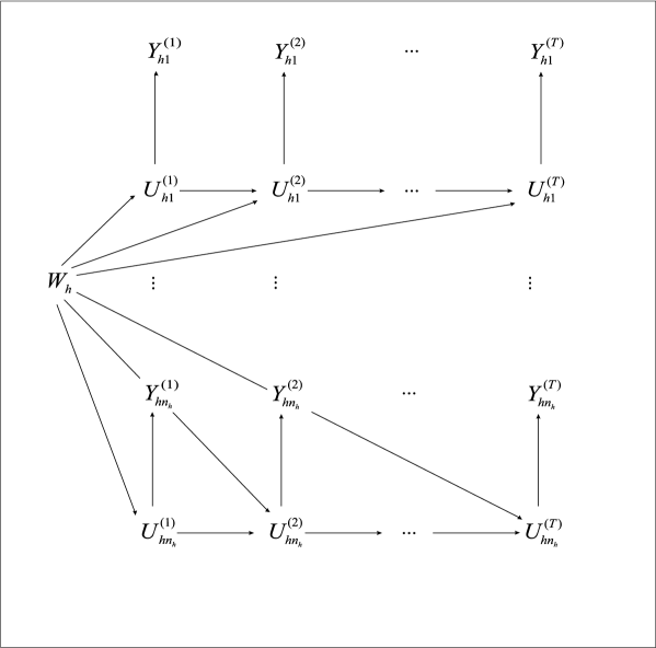
Figure 3: Path diagram for the multilevel LM model.

The above assumptions imply that, for every $h$, the response vectors $\mbox{\boldmath$Y$}_{h1},\ldots,\mbox{\boldmath$Y$}_{hn_{h}}$ are not independent, but they are conditionally independent given the latent variable $W_{h}$. Marginal independence holds between the vectors of response variables $\mbox{\boldmath$Y$}_{1},\ldots,\mbox{\boldmath$Y$}_{H}$ associated to the different clusters.

Model parameters are still the conditional response probabilities and the initial and transition probabilities of the latent process. The parameters of the first type are still denoted by $\phi_{y|u}^{(t)}$, $t=1,\ldots,T$, $u=1,\ldots,k$, $y=0,\ldots,l-1$, and correspond to $p(Y_{hi}^{(t)}=y|U_{i}^{(t)}=u)$; a similar notation is adopted in the multivariate case. An extended notation, which takes into account the multilevel structure, is instead necessary for the other parameters. In particular, for $w=1,\ldots,m$, we have $\pi_{u|w}=p(U_{hi}^{(1)}=u|W_{h}=w)$, $u=1,\ldots,k$, and $\pi_{v|uw}^{(t)}=p(U^{(t)}_{i}=v|U^{(t-1)}_{i}=u,W_{h}=w)$, $t=2,\ldots,T$, $u,v=1,\ldots,k$, $w=1,\ldots,m$. These parameters correspond, respectively, to the initial probabilities and the transition probabilities of the Markov chain associated to a subject belonging to a cluster with latent variable at level $w$. Finally, we also have to include the parameters for the distribution of each variable $W_{h}$, and then we let $\rho_{w}=p(W_{h}=w)$, $w=1,\ldots,m$.

Under the model assumptions, we can express, for each cluster $h$, the manifest distribution of the vector $\mbox{\boldmath$Y$}_{h}$ as

$$f_{h}(\mbox{\boldmath$y$})=p(\mbox{\boldmath$Y$}_{h}=\mbox{\boldmath$y$})=\sum_{w}p(\mbox{\boldmath$Y$}_{h}=\mbox{\boldmath$y$}|W_{h}=w)\rho_{w},$$ (31)

where $y$ has now the same dimension as $\mbox{\boldmath$Y$}_{h}$ and is made of the subvectors $\mbox{\boldmath$y$}_{i}$ of the same dimension as $\mbox{\boldmath$Y$}_{hi}$, $i=1,\ldots,n_{h}$. Moreover, we have that

$$p(\mbox{\boldmath$Y$}_{h}=\mbox{\boldmath$y$}|W_{h}=w)=\prod_{i}p(\mbox{\boldmath$Y$}_{hi}=\mbox{\boldmath$y$}_{i}|W_{h}=w),$$

where

$$p(\mbox{\boldmath$Y$}_{hi}=\mbox{\boldmath$y$}_{i}|W_{h}=w) = \sum_{u^{(1)}}\phi_{y_{i}^{(1)}|u^{(1)}}\pi_{u^{(1)}}\sum_{u^{(2)}}\phi_{y_{i}^{(2)}|u^{(2)}}^{(2)}\pi_{u^{(2)}|u^{(1)}}^{(2)}\cdots$$

$$\cdots\sum_{u^{(T)}}\phi_{y_{i}^{(T)}|u^{(T)}}^{(T)}\pi_{u^{(T)}|u^{(T-1)}}^{(T)}.$$

This probability may be efficiently computed through recursion (3).

5.2 Extension to include cluster and individual covariates and to the multivariate case

In the context of multilevel data, covariates are usually available at cluster and individual levels. Let $\mbox{\boldmath$z$}_{h}$ denote the column vector of available covariates for cluster $h$, let $\mbox{\boldmath$x$}_{hi}^{(t)}$ be the column vector of available covariates for subject $hi$ at occasion $t$, $h=1,\ldots,H$, $i=1,\ldots,n_{h}$, $t=1,\ldots,T$. These covariates are included in the model in a way similar to that illustrated in Section 4.2. Then we extend the notation by letting, for each subject $hi$, $\pi_{hi,u|w}=p(U_{hi}^{(1)}=u|W_{h}=w,\mbox{\boldmath$x$}_{hi}^{(1)})$, $u=1,\ldots,k$, and $\pi_{hi,v|uw}^{(t)}=p(U_{i}^{(t)}=v|U_{i}^{(t-1)}=u,W_{h}=w,\mbox{\boldmath$x$}_{hi}^{(t)})$, $t=2,\ldots,T$, $u,v=1,\ldots,k$, $w=1,\ldots,m$; we also let $\rho_{h,w}=p(W_{h}=w|\mbox{\boldmath$z$}_{h})$, $w=1,\ldots,m$, for each cluster $h$.

Covariates at cluster level are included into the model by adopting a suitable parametrization for the probabilities $\rho_{h,w}$. A natural choice is the multinomial logit parametrization, and then we assume

$$\log\frac{\rho_{h,w}}{\rho_{h,1}}=\gamma_{0w}+\mbox{\boldmath$z$}_{h}^{\prime}\mbox{\boldmath$\gamma$}_{1w},\quad w=2,\ldots,m,$$ (32)

where $\mbox{\boldmath$\gamma$}_{12},\ldots,\mbox{\boldmath$\gamma$}_{1m}$ are vectors of regression coefficients of the same dimension as $\mbox{\boldmath$z$}_{h}$, and $\gamma_{02},\ldots,\gamma_{0m}$ denote the corresponding intercepts.

A multinomial logit parameterization may also be adopted for the initial and transition probabilities of the Markov chain associated to every subject $hi$. However, if the conditional distribution of the response variables given the latent process is formulated so that the latent states are ordered, a considerable reduction of parameters is achieved by adopting a parametrizion based on global logits. This approach is exploited by Bartolucci et al., (2010), who relied on a Rasch parametrization for the distribution of each response variable given the corresponding latent state. Then, for the initial probabilities of every Markov chain they assume

$$\log\frac{\pi_{hi,u|w}+\cdots+\pi_{hi,k|w}}{\pi_{hi,1|w}+\cdots+\pi_{hi,u-1|w}}=\delta_{0w}+\delta_{1u}+(\mbox{\boldmath$x$}_{hi}^{(1)})^{\prime}\mbox{\boldmath$\delta$}_{2},\quad u=1,\ldots,k,\>w=2,\ldots,m,$$ (33)

where $\mbox{\boldmath$\delta$}_{2}$ is a vector of regression parameters of the same dimension as $\mbox{\boldmath$x$}_{hi}^{(t)}$ which is common to every level $u$. Moreover, the intercepts $\delta_{0w}$ depend on the level of $W_{h}$ (with $\delta_{01}\equiv 0$), and the intercepts $\delta_{1u}$ depend on the level of $U_{hi}^{(1)}$. We impose $\delta_{12}\leq\cdots\leq\delta_{1m}$ in order to ensure the invertibility of the global logit parametrization.

Finally, for what concerns the transition probabilities we have

$$\log\frac{\pi_{hi,v+1|uw}^{(t)}+\cdots+\pi_{hi,k|uw}^{(t)}}{\pi_{hi,1|uw}^{(t)}+\cdots+\pi_{hi,v-1|uw}^{(t)}}=\eta_{0w}+\eta_{1uv}+(\mbox{\boldmath$x$}_{hi}^{(t)})^{\prime}\mbox{\boldmath$\eta$}_{2},$$ (34)

with $u=1,\ldots,k$, $v=1,\ldots,k_{2}-1$, $w=1,\ldots,m$, and $t=2,\ldots,T$. As above, $\mbox{\boldmath$\eta$}_{2}$ is a vector of regression coefficients for the individual covariates, the intercepts $\eta_{0w}$ depend on the level of $W_{h}$ (with $\eta_{01}\equiv 0$), and the intercepts $\eta_{0uv}$ depend on the levels of $U_{hi}^{(t-1)}$ and $U_{hi}^{(t)}$ and must be decreasing ordered in $v$. These parameters may also be allowed to depend on the time occasion; for instance, we can have $\eta_{0v}^{(t)}$ in place of $\eta_{0v}$.

Finally note the extension of the model presented to the multivariate case, where we observe for every $hi$ and $t$ a vector of responses $\mbox{\boldmath$Y$}_{hi}^{(t)}$, is straightforward. The basic assumption to be added is that the variables in this vector are conditionally independent given the corresponding latent state $U_{hi}^{(t)}$. Bartolucci et al., (2010) also addressed this case, allowing for different sets of responses observed at each occasion. This assumption of conditional independence may also be relaxed by adopting a parametrization of type (28), including the lagged response variables as already discussed in Section 4.

5.3 Maximum likelihood estimation

Given an observed sample, the log-likelihood of the model illustrated above is given by

$$\ell(\mbox{\boldmath$\theta$})=\sum_{h}\log[f_{h}(\mbox{\boldmath$y$}_{h})],$$

where $\mbox{\boldmath$y$}_{h}$ is the vector containing the responses observed for all subjects in cluster $h$ and the manifest probability $f(\mbox{\boldmath$y$}_{h})$ is defined in (31).

The EM algorithm is again the mail tool we suggest to maximize $\ell(\mbox{\boldmath$\theta$})$. However, its implementation is more difficult with respect to the versions already illustrated for the presence of latent variables at two levels. First of all, for the case of univariate responses and considering the presence of covariates, the complete data log-likelihood may be expressed as

$$\ell^{*}(\mbox{\boldmath$\theta$}) = \sum_{h}\sum_{w}b_{h,w}\log(\rho_{h,w})+$$

$$+ \sum_{h}\sum_{i}\bigg{\{}\sum_{u}a_{hi,u}^{(1)}\log[\pi_{hi,u|w}^{(1)}]+$$

$$+ \sum_{u}\sum_{v}\sum_{t>1}a_{hi,uv}^{(t)}\log[\pi_{hi,v|uw}^{(t)}]+$$

$$+ \sum_{u}\sum_{t}\sum_{y}\tilde{a}_{hi,uy}^{(t)}\log[\phi_{y|u}^{(t)}]\bigg{\}},$$

where the dummy variables are defined as in Section 3.3 and $b_{h,w}$ is a dummy variable equal to 1 if cluster $h$ belongs to latent class $w$ (i.e. $W_{h}=w$).

At the E-step, we compute the conditional expected value of the above dummy variables given the observed data and the current value of the parameters; at the M-step, we maximize the conditional expected value of $\ell^{*}(\mbox{\boldmath$\theta$})$ obtained by substituting each dummy variable in (5.3) with the corresponding expected value obtained from the E-step. For details on the implementation of these steps we refer to Bartolucci et al., (2010).

6 Standard errors, model selection, and path prediction

In this section we show how to obtain standard errors for the model parameters, dealing in particular with the information matrix. We also outline the problem of model selection for what mainly concerns the choice of the number of latent states. Finally, we outline the problem of path prediction, i.e. how to find the maximum a posteriori sequence of latent states for a given subject.

6.1 Standard errors

It is well known that the EM algorithm, differently from other algorithms such as the Newton-Raphson or the Fisher-scoring, does not directly produce the information matrix of the model. This matrix is typically used for computing standard errors.

Several methods have been proposed to overcome this difficulty. Most of these methods have been developed within the literature on hidden Markov models; for a concise review see Lystig and Hughes, (2002). The more interesting methods are based on the information matrix obtained from the EM algorithm by the technique of Louis, (1982) or related techniques; see for instance Turner et al., (1998) and Bartolucci and Farcomeni, (2009). Other interesting methods obtain the information matrix on the basis of the second derivative of the manifest probability of the response variables by a recursion similar to (3); see Lystig and Hughes, (2002) and Bartolucci, (2006).

Among the method related to the EM algorithm, that proposed by Bartolucci and Farcomeni, (2009) is very simple to implement and requires a small extra code over that required for the maximum likelihood estimation. The method exploits a well-known result according to which the score of the complete data log-likelihood computed at the E-step of this algorithm corresponds to the score of the incomplete data log-likelihood. More precisely, we have

$$\mbox{\boldmath$s$}(\mbox{\boldmath$\theta$})=\frac{\partial\ell(\mbox{\boldmath$\theta$})}{\partial\mbox{\boldmath$\theta$}}=\left.\frac{\partial{\rm E}_{\bar{\mbox{\footnotesize\boldmath{$\theta$}}}}[\ell^{*}(\mbox{\boldmath$\theta$})|\mbox{\boldmath$Y$}]}{\partial\mbox{\boldmath$\theta$}}\right|_{\bar{\mbox{\footnotesize\boldmath{$\theta$}}}=\mbox{\footnotesize\boldmath{$\theta$}}},$$

where ${\rm E}_{\bar{\mbox{\footnotesize\boldmath{$\theta$}}}}[\ell^{*}(\mbox{\boldmath$\theta$})|\mbox{\boldmath$Y$}]$ denotes the conditional expected value of the complete-data log-likelihood computed at the parameter value $\bar{\mbox{\boldmath$\theta$}}$. Then, the observed information matrix, denoted by $\mbox{\boldmath$J$}(\mbox{\boldmath$\theta$})$, is obtained as minus the numerical derivative of $\mbox{\boldmath$s$}(\mbox{\boldmath$\theta$})$. The standard error of each parameter estimate is then obtained as the square root of the corresponding diagonal element of $\mbox{\boldmath$J$}(\hat{\mbox{\boldmath$\theta$}})^{-1}$. These standard errors may be used for hypothesis testing and for obtaining confidence intervals in the usual way.

The information matrix can also be used for checking local identifiability at $\hat{\mbox{\boldmath$\theta$}}$. We consider the model to be local identifiable if the matrix $\mbox{\boldmath$J$}(\hat{\mbox{\boldmath$\theta$}})$ is of full rank. See also McHugh, (1956) and Goodman, (1974).

6.2 Model Choice

In applying a LM model, a fundamental problem is that of the choice of the number of latent states, denoted by $k$. For multilevel versions of this model, it is also necessary to choose the number of support points for the latent variables at cluster level, denoted by $m$.

In order to choose the above quantities, it is natural to use information criteria such as the Akaike Information Criterion (AIC), see Akaike, (1973), and the Bayesian Information Criterion (BIC), see Schwarz, (1978). According to first criterion, we choose the number of states corresponding to the minimum of $AIC=-2\ell(\hat{\mbox{\boldmath$\theta$}})+2g$, where $g$ is the number of non-redundant parameters; according to the second, we choose the model with the smallest value of $BIC=-2\ell(\hat{\mbox{\boldmath$\theta$}})+g\log(n)$.

The performance of the two approaches above have been deeply studied in the literature on mixture models; see McLachlan and Peel, (2000), Chapter 6. These criteria have also been studied in the hidden Markov literature for time series, where the two indices above are penalized with a term depending on the number of time occasions; see Boucheron and Gassiat, (2007). From these studies, it emerges that BIC is usually preferable to AIC, as the latter tends to overestimate the number of latent states.

The theoretical properties of AIC and BIC applied to the LM models are less studied. However, BIC is a commonly accepted model choice criterion even for these models. It has been applied by many authors, such as Langeheine, (1994), Langeheine and Van de Pol, (1994), and Magidson and Vermunt, (2001). In particular, Bartolucci et al., (2009) suggested the use of this criterion together with that of diagnostic statistics measuring the goodness-of-fit and goodness-of-classification, whereas a simulation study may be found in Bartolucci and Farcomeni, (2009).

6.3 Path prediction

Once the model has been estimated, a relevant issue is that of path prediction, i.e. finding the most likely sequence of latent states for a given subject on the basis of the responses he/she provided. For the $i$th subject in the sample, this is the sequence $\hat{\mbox{\boldmath$u$}}_{i}=(\hat{u}_{i}^{(1)},\ldots,\hat{u}_{i}^{(T)})$ such that

$$p(\hat{\mbox{\boldmath$u$}}|\mbox{\boldmath$y$}_{i})=\max_{\mbox{\footnotesize\boldmath{$u$}}}p(\mbox{\boldmath$u$}|\mbox{\boldmath$y$}_{i}),$$

where we use the notation of Section 2. This definition may be simply adapted to more general cases involving individual covariates and/or multilevel data.

The problem above is different from that of finding the most likely state occupied by a subject at certain occasion. This problem may be simply solved on the basis of the posterior probabilities of type $r^{(t)}(u|\mbox{\boldmath$y$})$, whose computation is required within the EM algorithm; see Section 2.3. In any case, we can use an efficient algorithm which avoid the evaluation of the posterior probability $p(\mbox{\boldmath$u$}|\mbox{\boldmath$y$})$ for every configuration $u$ of the latent process. This is known as Viterbi algorithm (Viterbi,, 1967; Juang and Rabiner,, 1991), and is illustrated in the following.

For a given subject $i$ with response configuration $\mbox{\boldmath$y$}_{i}=(y_{i}^{(1)},\ldots,y_{i}^{(T)})$, let ${\tilde{r}}_{i}^{(1)}(u)=p(U_{i}^{(1)}=u,y_{i}^{(1)})$ and, for $t=2,\ldots,T$, let

$${\tilde{r}}_{i}^{(t)}(u)=\max_{u^{(1)},\ldots,u^{(t-1)}}p(U_{i}^{(1)}=u^{(1)},\ldots,U_{i}^{(t-1)}=u^{(t-1)},U_{i}^{(t)}=u,y_{i}^{(1)},\ldots,y_{i}^{(t)}).$$

A forward recursion can be used to compute the above quantities, and a backward recursion based on these quantities can then be used for path prediction:

1. for $u=1,\ldots,k$ compute $\tilde{r}^{(1)}_{i}(i)$ as $\pi_{u}p(y^{(1)}_{i}|U^{(1)}_{i}=u)$;

2. for $t=2,\ldots,T$ and $v=1,\ldots,k$ compute ${\tilde{r}}^{(t)}_{i}(v)$ as

   $$p(y_{i}^{(t)}|U^{(t)}_{i}=v)\>\max_{u}[{\tilde{r}}^{(t-1)}_{i}(u)\pi_{uv}^{(t)}];$$

3. find the optimal state $\tilde{u}^{(T)}_{i}$ as $\hat{u}^{(T)}_{i}=\arg\max_{u}\tilde{r}^{(T)}_{i}(u)$;

4. for $t=T-1,\ldots,1$, find $\hat{u}_{i}^{(t)}$ as $\tilde{u}^{(t)}_{i}=\arg\max_{u}\tilde{r}^{(t)}_{i}(u)\pi_{u\hat{u}_{i}^{(t+1)}}$.

All the above quantities are computed on the basis of the ML estimate of the parameter $\theta$ of the model of interest.

7 Empirical illustrations

In order to illustrate the approaches reviewed in this paper, we provide a synthetic overview of some interesting applications appeared in the literature. We describe different datasets, the aspects involved in practically fitting and using the LM models, and the interpretation of the results.

7.1 Marijuana Consumption dataset

The univariate version of the LM model described in Section 2.1 was applied by Bartolucci, (2006) to analyze a marijuana consumption dataset based on five annual waves of the “National Youth Survey” (Elliot et al.,, 1989). The dataset concerns $n=237$ respondents who were aged 13 years in 1976. The use of marijuana was measured through five ordinal variables, one for each annual wave, with three categories corresponding to: “never in the past”, “no more than once in a month in the past year”, and “once a month in the past year”. The substantive research question is whether there is an increase of marijuana use with age.

Using BIC, Bartolucci, (2006) selected an LM model with three latent states, homogeneous transition probabilities, and a parsimonious parameterization for the measurement model based on global logits, which recalls that in (14). This parametrization is based on one parameter for each latent state, which may be interpreted as the tendency to use marijuana for a subject in this state, and one cutpoint for each response category. Then, the latent states may be ordered representing subjects with “no tendency to use marijuana”, “incidental users of marijuana”, and “subjects with high tendency to use marijuana”. Also note that the cutpoints are common to all the response variables, since these variables correspond to repeated measurements of the same phenomenon under the same circumstances. This is because the dynamics of the marijuana consumption is only ascribed to the evolution of the underlying tendency of this consumption.

Bartolucci, (2006) also tested different hypotheses on the transition matrix of the latent process. In particular, he found that the hypothesis that the transition matrix has a tridiagonal structure, i.e.

$$\mbox{\boldmath$\Pi$}^{(t)}=\pmatrix{1-\delta_{1}&\delta_{1}&0\cr\delta_{2}&1-(\delta_{2}+\delta_{3})&\delta_{3}\cr 0&1-\delta_{4}&\delta_{4}},$$

cannot be rejected. This hypothesis implies that the transition from state $u$ to latent state $v$ is only possible when $v=u-1$ or $v=u+1$.

The results under the selected LM model say that, at the beginning of the period of observation, the 89.6% of the sample is in the first class (lowest tendency to marijuana consumption) and the 1.5% is in the third class (highest tendency to marijuana consumption). An interesting interpretation of the pattern of consumption emerges from the estimated transition matrix. A large percentage of subjects remains in the same latent class, but almost 25% of accidental users switches to the class of high frequency users. From the estimated marginal probabilities of the latent classes emerge that the tendency to use marijuana increases with age, since the probability of the third class increases across time.

7.2 Educational dataset

An interesting illustration of an LM model with individual covariates was given by Vermunt et al., (1999). They used data from an educational panel study conducted by the “Institute for Science Education in Kiel (Germany)” (Hoffmann et al.,, 1985). A cohort of secondary school pupils was interviewed once a year from grade 7 to grade 9 with respect to their interests in physics as a school subject. The response variables have been dichotomized with categories “low” and “high” to avoid sparseness of the observed frequency table. Based on these data, the LM model is used to draw conclusions on whether interest in physics depends on the interest in the previous period of observation and on two available covariates: sex and grade in physics at the present time.

Vermunt et al., (1999) estimated a univariate LM model with both initial and transition probabilities of the latent process depending on the available covariates according to a multinomial logit parametrization. In this model, the measurement error was constrained to be the same for all time points, meaning that the conditional distribution of the response variables given the latent state is the same for every occasion. Then, they relaxed some of the basic assumptions of the LM model, such as the assumption that the Markov chain is first-order.

According to the parameter estimates of the selected model, there is a significant effect of sex and grade on the interest in physics. Pupils with higher grades are more interested in physics than pupils with lower grades, girls are less interested in physics than boys. Moreover, the interest has a positive effect on the grade at the next time occasion. For the boys, the probability of switching from “low” to “high interest” is larger than that for girls, as well as to keep their interest high.

7.3 Criminal dataset

The multivariate version of the LM model where both the initial and the transition probabilities of the latent process depend on time-constant covariates was illustrated by Bartolucci et al., 2007b . They analyzed the conviction histories of a cohort of offenders who were born in England and Wales in 1953. The offenders were followed from the age of criminal responsibility, 10 years, until the end of 1993. They were grouped in 10 major categories and gender was included in the model as explanatory variable. The analysis was based on $T=6$ age bands: 10-15, 16-20, 21-25, 26-30, 31-35 and 36-40 years.

The adopted LM model allows to estimate trajectories for behavioral types which are determined by the criminal conviction grouping. It also allows to give rise to a general population sample by augmenting the observed sample with not-convicted subjects.

According to Bartolucci et al., 2007b , the fit of the model is considerably improved by relaxing the assumption of homogeneity of the latent Markov chain, but retaining the constraint that males and females have the same transition probabilities. In particular, they selected a model based on partially homogeneity, as described in Section 3.2; equation (20). Therefore there are two transition probability matrices: the first for transitions up to time $\bar{t}$ and the second from time $\bar{t}$ and beyond. The choice of $\bar{t}=2$ has been made on the basis of the BIC.

In summary, the selected model is based on a partially homogeneous Markov chain with five latent states, different initial and equal transition probabilities for males and females. From the estimated conditional probabilities of conviction for any offence group and any latent state, it was possible to determine classes of criminal activity. In accordance to the typologies found in the criminological latent class literature, these classes are interpreted as: “non-offenders”, “incidental offenders”, “violent offenders”, “theft and fraud offenders” and “high frequency and varied offenders”.

The estimated initial probabilities show that in the first age band the percentage of males who are incidental offenders is higher than that of females. The common estimated transition probabilities for males and females from age band 10-15 to age band 16-20, and from one age band to the others for offenders over 16, show that the first transition occurs at an early age, 16 years, which in western society represents the peak of the age-crime curve.

At the first time occasions, “incidental offenders” have a quite high probability of persistence when moving from the age band 10-15 to age band 16-20. Moreover, “theft and fraud offenders” are mainly females and they have a high chance of moving to the class of non-offenders. The “high frequency and varied offenders” are mainly males and they have a high persistence.

The estimated transition probabilities from age band 16-20 to the subsequent age bands show that the subjects belonging to the latent state of “non-offenders” have a very low chance of becoming offenders; “theft and fraud offenders” and “violent offenders” have a high probability of dropping out of crime. From the estimated proportion of males and females in each latent state at every time occasion it can be seen that 7% of males are “violent offenders” at age 16-20 years and 32% are “incidental offenders” at the same age. Only 3% of females are “theft and fraud offenders” at age 16-20 years.

7.4 Dataset on financial products preferences

An interesting analysis of data obtained from face to face interviews of the household ownership of 12 financial products was offered by Paas et al., (2009). The panel was conducted by a market research company among 7676 Dutch households in 1996, 1998, 2000 and 2002. To have an accurate representation of the products portfolio, the households were asked to retrieve their bank and insurance records in order to check which product they owned. Households that dropped out were replaced to ensure the representativeness of the sample for the population with respect to demographic variables, such as age, income and marital status.

The aim of the study was to get insights on the developments of the individual household product portfolio and the effect of demographic covariates on such development. It also concentrates on predicting future behaviors of acquisition.

The authors proposed to use a time homogeneous multivariate LM model, with time-varyng covariates affecting the latent process as in Section 4.2. They added additional assumptions to the model, such as constant conditional probabilities of the response variables given the latent process. This is done to avoid manifest changes, so that the product penetration levels are consistent in latent states over measurement occasions. Moreover, they formulated the model with a time-constant effect of the covariates on the transition probabilities.

The model selected on the basis of BIC is based on nine latent states. These states can be ordered according to increasing penetration levels across the analyzed products, which range from bonds, the most commonly owned product, to saving accounts. The results highlight some divergences from common order of acquisitions, such as the acquisition of a mortgage before owing a credit card or viceversa. Loans and unemployment insurance are most often acquired. According to the estimated transition matrix there is a high persistence in the same latent state: only 14% of the households changed latent state in the period of the study. The most common switch is from latent class 7 to 8, where latent state 7 is characterized by the acquisition of mortgage, life insurance, pension fund, car insurance, and saving accounts, whereas latent state 8 for all the previous products plus the credit card. Another common switch is from latent state 4 to 7, where the first is characterized by the acquisition of life insurance, pension fund, car insurance, and savings accounts. This means that multiple products were acquired between consecutive measurement occasions.

Income, age of the head of the household, and household size have a significant effect on the initial and transition probabilities according to the Wald test. The covariate values implying a larger probability of belonging to an initial latent class also imply a greater probability of switching into the same latent class. For example larger households are relatively often found in latent states where overall product ownership probabilities are relatively low.

The prediction of future purchase of a financial product was performed on the basis the posterior latent state membership probabilities for each household at the last occasion $T$, given all other observed information. To assess the accuracy of the forecasting, the authors used the Gini coefficient as a measure of concentration. Considering the empirical results in the last wave referred to year 2002, which was not considered when estimating the model, the authors showed that, for most products, the prediction equations are effective for forecasting household acquisition.

7.5 Job position dataset

The multivariate LM model with covariates affecting the manifest probabilities proposed by Bartolucci and Farcomeni, (2009) was applied by these authors to data extracted from the “Panel Study of Income Dynamics” database (University of Michigan). These data concern $n=1446$ women who were followed from 1987 to 1993. The binary response variables are fertility, indicating whether a woman had given birth to a child in a certain year and employment, indicating whether she was employed. The covariates are: race (dummy variable equal to 1 for a black woman), age (in 1986), education (year of schooling), child 1-2 (number of children in the family aged between 1 and 2 years, referred to the previous year), child 3-5, child 6-13, child 14-, income of the husband (in dollars, referred to the previous year).

The main issue concerns the direct effect of fertility on employment. Also of interest are the strength of the state dependence effect for both response variables and how these variables depend on the covariates.

Bartolucci and Farcomeni, (2009) used an LM model with covariates affecting the manifest probabilities since they were interested in separately estimating the effect of each covariate on each outcome. The proposed LM model allows to separate these effects from the unobserved heterogeneity, by modeling the latter with a latent Markov process. In this way, unobserved heterogeneity effects on the response variables are allowed to be time-varying; this is not allowed neither within a LC model with covariates nor in the most common random effect models.

The model selected using AIC and BIC is with three latent states. Under this model, race has a significant effect on fertility, but not on employment according to the estimates of the parameters affecting the marginal logits of fertility and employment and the log-odds ratio between these variables. Age has a stronger effect on fertility than on employment. Education has a significant effect on both fertility and employment, whereas the number of children in the family strongly affects only the first response variable and income of the husband strongly affects only the second one.

The log-odds ratio between the two response variables, given the latent state, is negative and highly significant, meaning that the response variables are negatively associated when referred to the same year. On the other hand, lagged fertility has a significant negative effect on both response variables and lagged employment has a significant effect, which is positive, on both response variables. Therefore, fertility has a negative effect on the probability of having a job position in the same year of the birth, and the following one. Employment is serially positively correlated (as consequence of the state dependence effect) and fertility is negatively serially correlated.

From the estimates of the support points for each latent state it may be deduced that the latent states correspond to different levels of propensity to give birth to a child and to have a job position. The first latent state corresponds to subjects with the highest propensity to fertility and the lowest propensity to have a job position. On the contrary, the third latent state corresponds to subjects with the lowest propensity to fertility and the highest propensity to have a job position. Finally, the second state is associated to intermediate levels of both propensities. The two propensities are negatively correlated.

Overall, it results that the 78.5% of women started and persisted in the same latent state for the entire period, whereas for the 21.5% of women had one or more transitions between states. The presence of these transitions is in accordance to the rejection of the hypothesis that a LC model is suitable for these data.

7.6 Dataset on anorectic patients

An interesting extension of the model to account for a hierarchical structure has been recently proposed by Rijmen et al., (2007). They illustrated the model by a novel application using a data set from an ecological momentary assessment study (Vansteelandt et al.,, 2007) on the course of emotions among anorectic patients. At nine occasions for each of the seven days of observations, 32 females with eating disorders received a signal and were asked to rate themselves on a 7-point scale with respect to the intensity with which they experienced 12 emotional states. These were taken from the following emotional categories: “anger and irritation”, “shame and guilt”, “anxiety and tension”, “sadness and loneliness”, “happiness and joy”, “love and appreciation”. The response has been dichotomized (0-2 vs. 3-6) and the signal has been considered equally spaced. The aim of the study was to detect the course of emotion among the patients.

As a preliminary analysis, Rijmen et al., (2007) used the univariate version of the LM model without covariates. They treated each person by day combination as a separate case assuming that the data stemming from different days were independent and that the parameters were constant over days. On the basis of such model the authors selected four latent states. The first state is interpreted as positive mood, the third as negative mood, the second as low intensity for all emotions except tension, and the fourth as neutral to moderately positive mood. According to the estimated transition matrix there is high persistence in the same state. The probability of moving from state 1 to state 2 is 0.14, from state 3 to 4 is 0.18 and from state 4 to 3 is 0.14 . They noted that there is an indirect transition from state 3 to state 1 via the emotionally more neutral state 4. Over the days there is an increase of the marginal probabilities of states 1 and 4 indicating that the mood of patients tends to become better later on in the day.

Rijmen et al., (2007) also used a hierarchical LM model by introducing a latent variable at day level to account for the fact that data stemming from different days are not independent. They modeled the transition between latent states at day and signal levels by a first-order time homogeneous Markov chain. They estimated a model with two states at the day level and two signal states within each day-state. For the first day state, the signal state 1 is characterized by high probabilities of experiencing positive emotions and low probabilities of negative emotions. Therefore this state is interpreted as positive mood. Instead the second day state is interpreted as negative mood. In the signal state 2 positive emotions are not well separated from negative emotions and the state is considered as an emotionally neutral to moderately positive state. A tendency to experience more positive emotions emerges from the estimated initial and conditional probabilities of the chain over day and signal.

7.7 Dataset on student math achievement

A multilevel version of the latent Markov model was applied by Bartolucci et al., (2010) to analyze how the cognitive math achievement changes over time of schooling. Multilevel models are standard tools for the analysis of such kind of data as they allow to explicitely consider a hierarchical structure such as students nested in classes and schools.

The data derived from the repeated administration of test items to students attending public and non-public middle schools in an Italian Region. A set of dichotomously scored items was administered at the end of each of the three years of school (28 at the end of the first year, 30 at the end of the second, and 39 at the end of the third year) to 1,246 students who progressed from Grade 6 to Grade 8. They are from 13 public and 7 non-public middle schools. The recorded social background characteristics of the students are father’s and mother’s education. The school characteristics are: number of students, number of teachers, students-teachers ratio, and years since school opened.

The main issue concerns the evaluation of the performance of schools, measured in terms of achievement attained by pupils at the end of the period of formal schooling. The proposed approach takes into account imperfect persistence of achievement, heterogeneity in learning and measurement error in test scores contributing to get an unbiased estimate of the added value of public and non-public schools.

On these data the authors fitted a multilevel LM model for multivariate data with a structure similar to that presented in Section 5. On the basis of the BIC, they selected the model based on $m=4$ support points for the latent variable at cluster level and $k=6$ states for the latent Markov chain at individual level. Each latent state is associated to an estimated the ability level, so that these states can easily identify the group of the most proficient students and that of the least proficient students. The ordered estimated conditional probabilities for each latent class and each set of items administered at each grade show that the difficulty of the items is increasing over time and they allow to identify the items which are tailored to distinguish less capable students.

The estimates of the intercepts and the regression coefficients for the logistic model at cluster level based on parametrization (32) allowed interpretation of the four cluster latent classes. The class of cluster $D$ is mainly characterized by the non-public schools with less than 18 years since school opened and with a ratio between students and teachers smaller than 8. As the value of the covariate “ratio between student and teachers” increases there is more chance that the class is of type A rather than of type B. As the value of the year of activity of the school increases there is more chance that the class is of type A rather than of type B.

The estimated parameters of the global logits defined on the initial and transition probabilities are interpreted on the basis of formulae (33) and (34). According to them the classes of those schools belonging to type $B$ are less helpful in increasing math ability in the first year of the middle school, as compared to the classes of the other clusters. The same classes contribute less also from Grade 6 to Grade 7 but they contribute the most to student’s math ability from Grade 7 to 8. The ability of the students increases for those having highly educated fathers. The magnitude of this increase is stronger at Grade 6 compared to the other grades. They identify how the covariates related to each class affect the probability that this class is of type A, B, C or D. The most interesting conclusion is that classes of students in public schools are mostly of type A (32%), B (23%), and C (38%), whereas those in non-public schools are only of type A (79%) and D (21%). The estimated regression coefficients related to the individual covariates show that the ability of the students increases for those having higher educated fathers.

8 Conclusions and further developments

In this paper we presented a review of the latent Markov model which starts with the basic model of Wiggins, (1973), for both univariate and multivariate data. We also illustrated extensions to the inclusion of covariates and to multilevel data, and outlined maximum likelihood estimation and related inferential methods. We tried to keep the presentation simple and provide references to methods which are of easy implementation, taking ideas from methods widely applied in the literature on hidden Markov models for time series. Moreover, in order to retain a simple presentation we dealt with the case of balanced data in which all subjects are observed at the same number of occasions, the same response variables are obtained at every occasion, and there are no missing responses.

The potentialities of the LM approach are illustrated by summarizing the results of several applications available in the literature. It is worth noting that the number of applications available in the literature is growing; recent applications also involve situations which are not typically those of longitudinal data. Examples concern the estimation of closed-populations on the basis of capture-recapture data (Bartolucci and Pennoni,, 2007) and the assessment of the peer review process of grant applications (Bornmann et al.,, 2008).

In this section we would like to summarize further developments of the LM models that, in our opinion, deserve particular attention:

• More flexible parametrizations for the conditional distribution of the response variables given the latent process: We refer in particular to parameterizations which address the problem of multidimensionality when the model is applied, for instance, to data coming from the administration of test items assessing different types of ability. This is a problem well known in the Item Response Theory, which may concern different fields of applications such as psychology and assessment of the quality of life. Flexible parameterizations are also of interest when the response variables are of mixed nature; for instance, we may have a mixture of binary, ordinal, and continous variables.

• Higher-order Markov chains: the assumptions that the latent Markov chain if of first-order may be restrictive when there is “memory effect” such that the latent state of a subject at a given occasion depends on two or more previous occasions. The extension to second or higher-order Markov chains is rather simple to implement and has been already applied in certain contexts. However, to our knowledge, a systematic illustration of this higher-order approach does not seem to be available in the literature.

• Missing responses: It is well known that longitudinal datasets typically suffer from the problem of missing responses due to several reasons. In applying an LM model, a trivial solution to this problem consists in eliminating from the sample subjects with at least one missing response. Obviously, this solution may lead to a strong bias of the parameter estimates when the assumption that these responses are missing at random is not plausible. The interest here is in formulating LM models in which the event of missing response is explicitly modeled given the latent state and the evolution of the latent process takes into account this possibility by adopting a suitable parametrization of the transition matrices.

• Multilevel data with evolution at cluster level: We presented in Section 5 a multilevel extension of the LM model in which only one latent variable is used to represent the effect of each cluster. However, this effect may have its own dynamics as the effect at individual level. Hence, of interest is the extension in which a sequence of occasion-specific latent variables is used to model the effect of each cluster. The resulting model may then be formulated by assuming the existence of two nested latent Markov chains. Given the chain at cluster level, another chain is associated to each individual in the cluster. This model if of particular interest, but it seems difficult to provide a simple method for maximum likelihood estimation, given the difficulty of obtaining the manifest distribution of the response variables.

References

- Akaike, (1973) Akaike, H. (1973). Information theory as an extension of the maximum likelihood principle. In Petrov, B. N. and F., C., editors, Second International symposium on information theory, pages 267–281, Budapest. Akademiai Kiado.
- Altman, (2007) Altman, R. M. (2007). Mixed hidden Markov models: an extension of the hidden Markov model to the longitudinal data setting. Journal of the American Statistical Association, 102:201–210.
- Anderson, (1954) Anderson, T. W. (1954). Probability models for analysing time changes in attitudes. In press, T. F., editor, Mathematical Thinking in the Social Science. Lazarsfelsd P. F.
- Archer and Titterington, (2009) Archer, G. E. B. and Titterington, D. M. (2009). Parameter estimation for hidden Markov chains. Journal of Statistical Planning and Inference, 108:365–390.
- Bartolucci, (2006) Bartolucci, F. (2006). Likelihood inference for a class of latent Markov models under linear hypotheses on the transition probabilities. Journal of the Royal Statistical Society, series B, 68:155–178.
- Bartolucci and Besag, (2002) Bartolucci, F. and Besag, J. (2002). A recursive algorithm for Markov random fields. Biometrika, 89:724–730.
- (7) Bartolucci, F., Colombi, R., and Forcina, A. (2007a). An extended class of marginal link functions for modelling contingency tables by equality and inequality constraints. Statistica Sinica, page in press.