Entanglement distillation from quasifree Fermions.

Abstract

We develop a scheme to distill entanglement from bipartite Fermionic systems in an arbitrary quasifree state. It can be applied if either one system containing infinite one-copy entanglement is available or if an arbitrary amount of equally prepared systems can be used. We show that the efficiency of the proposed scheme is in general very good and in some cases even optimal. Furthermore we apply it to Fermions hopping on an infinite lattice and demonstrate in this context that an efficient numerical analysis is possible for more than $10^{6}$ lattice sites.

1 Introduction

An important class of Fermionic states are the Gaussian ones. They describe equilibrium states of quasifree spin chains, such as non-interacting electrons [16]. Since they are completely characterized by their two-point correlations, they are under good control also in case of large particle number. For an example of their standard description based on a fixed basis in the Fermionic Fock space, see [7].

Defining entanglement is not straightforward in Fermionic systems as Fermions are indistinguishable and described by antisymmetric tensor products. There are several ways around this problem. E.g. in [11] antisymmetrized states with definite particle number are studied while in [1] the focus is on the lattice spin system admitting Fermionic description. The conceptionally clearest approach is, however, to base the description of subsystems not on tensor products of Hilbert spaces, but on the notion of local observables [9]. This approach is successfully applied to the study of entanglement of systems with infinite degrees of freedom [20, 13] and for the analysis of separable [17] and maximally entangled [18] states of Fermionic systems. Furthermore, the conservation of local parity superselection rule allows for different possible definitions for separability [5] (consult that article also for more literature on Fermionic entanglement).

In this paper we will take an operational point of view. Instead of asking how much entanglement is contained in a given bipartite, Fermionic system, we will look for explicit distillation protocols, i.e. procedures to generate (in terms of LOCC), from a number of Fermions, pairs of distinguishable particles in a maximally entangled state. The asymptotic rate of such a protocol can then be regarded as a measure for the entanglement contained in the original state. The advantage of this approach is that the only concept which needs a (slight) generalization is that of local operations (of bipartite Fermionic systems and from a Fermionic to an ordinary bipartite system). The latter, however, can be easily based on the idea of local observables mentioned in the last paragraph; cf. [12] for a more complete discussion.

Following this idea, we present a family of protocols which is particularly adopted towards distillation from quasifree (i.e. Gaussian) states. The general structure involves a two step procedure: First we generate (with a certain success probability $p$) bipartite $d$-level systems (where the local dimension can be chosen within a certain range) in an isotropic state $\sigma$. In particular for very large systems (cf. the discussion of free Fermions on an infinite lattice in Section 8) the entanglement fidelity of $\sigma$ can be already very close to one such that no more steps are necessary. If this is not the case but $\sigma$ is distillable we can continue with standard techniques like the recurrence method or hashing (cf. [21] and the references therein).

Each protocol in this family admits a very easy parametrization in terms of two operators (a projection $D$ and a partial isometry $V$; cf. Section 4) on the one-particle reference space $\mathcal{K}$ rather than the corresponding Fermionic Fockspace $\mathcal{H}$. This implies in particular that we can express the success probability $p$ and the fidelity $f$ of the isotropic output states $\sigma$ (from which the overall rate of the protocol can be calculated with known formulas, once we have decided how to process the resulting $d$-level systems) in terms of $D$ and $V$. The dimension of $\mathcal{K}$ (i.e. the space on which $D$ and $V$ operate) grows, however, only linearly in the system size (i.e. the number of independent modes) while $\dim\mathcal{H}$ grows exponentially. Hence we get a very efficient way to discuss the entanglement content of quasifree Fermionic systems which is applicable to, literally, millions of particles. This is explicitly demonstrated in Section 8.

The given class of protocols is still large and for a given quasifree state $\rho_{S}$ (which is completely described by its two-point correlation matrix $S$) most of them lead to very poor results. Therefore, in Section 5 we present a scheme to derive the operators $D$ and $V$ from $S$. It is based on the observation that to any generic, quasifree state $\rho_{S}$ we can associate a quasifree, maximally entangled state in a natural way (this resembles a little bit the Schmidt decomposition, but note that pureness of $\rho_{S}$ is not required). For a large subset of quasifree states (whose dimension grows quadratically in the system size) this particular protocol optimizes the product of success probability $p$ and fidelity $f$ (we will discuss in Section 5 why this is a good figure of merit and, actually, related to the overall distillation rate).

The presented scheme is discussed in terms of two classes of examples: Small systems consisting of two or four modes and free Fermions, hopping on a one-dimensional lattice. The numerical efficiency mentioned above allows us in the latter case to treat large particle numbers and this leads to new insights about the entanglement properties of this particular system, which are interesting in their own right.

The paper is organized as follows: In Section 2 we will start with some mathematical preliminaries about Fermionic systems. The approach we present here is based on the “selfdual formalism” [3, 2] and might be unfamiliar for most readers (although it is not particularly new). For the purposes of this paper it is, however, the most natural formalism. In Section 3 we apply it to discuss some aspects of bipartite Fermionic systems and in Section 4 we present the family of protocols mentioned above. The question of optimality is then treated in Section 5. The rest of the paper is finally devoted to examples: two and four modes in Section 6 and 1d lattice systems in Sections 7 and 8. Several technical aspects (including, in particular, proofs) are postponed to the appendix.

2 Mathematical preliminaries

To introduce some terminology and notations, let us start with some technical remarks about Fermionic systems. All the material we are going to present here can be found in the literature, [3, 2] are some standard references.

A Fermionic system consisting of $n$ modes can be described by smeared Majorana fields

$$\mathcal{K}^{(n)}\ni x\mapsto B(x)\in\mathcal{B}(\mathcal{H}^{(n)}).$$ (1)

The system Hilbert space $\mathcal{H}^{(n)}$ is $2^{n}$ dimensional and can be realized as the Fermionic Fockspace over $\mathbb{C}^{n}$. Therefore we will refer to it occasionally as the Fermionic Fock space of $n$ modes although the precise form of $\mathcal{H}^{(n)}$ is (apart from its dimension) not really important. The Hilbert space $\mathcal{K}^{(n)}$ – in the following called reference space – is $2n$ dimensional and equipped with an antilinear involution (called complex conjugation) $J:\mathcal{K}^{(n)}\rightarrow\mathcal{K}^{(n)}$. In other words $J$ satisfies

$$J(x+\lambda y)=J(x)+\bar{\lambda}J(y),\quad J^{2}={\leavevmode{\rm 1\mkern-4.8muI}}$$ (2)

for all $x,y\in\mathcal{K}^{(n)}$ and all $\lambda\in\mathbb{C}$. The typical choice for $\mathcal{K}^{(n)}$ and $J$ is $\mathbb{C}^{2n}$ equipped with the ordinary conjugation in the canonical basis. As with $\mathcal{H}^{(n)}$, however, the explicit realization of $(\mathcal{K}^{(n)},J)$ is not important. $\mathcal{K}^{(n)}$ contains a distinguished real subspace given by

$$\mathcal{K}^{(n)}_{\mathbb{R}}=\{x\in\mathcal{K}^{(n)}\,|\,Jx=x\}\subset\mathcal{K}^{(n)}.$$ (3)

Lots of structures we will encounter in the following are actually associated to $\mathcal{K}_{\mathbb{R}}^{(n)}$ rather than to $\mathcal{K}^{(n)}$. We will call in particular an orthonormal basis $e_{j}$, $j=1,\dots,2n$ of $\mathcal{K}_{\mathbb{R}}^{(n)}$ (which is of course an orthonormal basis of $\mathcal{K}^{(n)}$, too) a real basis.

The operators $B(x)$ are (complex) linear in $x\in\mathcal{K}^{(n)}$ satisfy the canonical anticommutation relations (CAR) in the form

$$\{B(x),B(y)\}=\langle Jx,y\rangle{\leavevmode{\rm 1\mkern-4.8muI}},\quad B(x)^{*}=B(Jx)$$ (4)

and they act irreducibly on $\mathcal{H}^{(n)}$, i.e.

$$[A,B(x)]=0\ \forall x\in\mathcal{K}^{(n)}\Rightarrow A=\lambda{\leavevmode{\rm 1\mkern-4.8muI}}.$$ (5)

These conditions fix the $B(x)$ up to unitary equivalence, which is the reason why we are not interested in their explicit form. They can be constructed easily in terms of ordinary creation and annihilation operators. The details are shown in Appendix A.

Let us consider now states of the system. To any density operator $\rho$ on $\mathcal{H}^{(n)}$ we can associate a covariance operator $S\in\mathcal{B}(\mathcal{K}^{(n)})$ by

$$\operatorname{tr}(\rho B(x)B(y))=\langle Jx,Sy\rangle\quad\forall x,y\in\mathcal{K}.$$ (6)

$S$ is selfadjoint and satisfies

$$0\leq S\leq{\leavevmode{\rm 1\mkern-4.8muI}}\ \text{and}\ JSJ={\leavevmode{\rm 1\mkern-4.8muI}}-S.$$ (7)

A state $\rho_{S}$ is called quasifree if it is uniquely characterized by $S$ and the conditions

$$\operatorname{tr}(\rho_{S}B(x_{1})\cdots B(x_{2l+1}))=0$$ (8)

$$\operatorname{tr}(\rho_{S}B(x_{1})\cdots B(x_{2l}))=\sum\operatorname{sign}(p)\prod_{j=1}^{l}\langle Jx_{p(2j-1)},Sx_{p(2j)}\rangle,$$ (9)

which have to hold for all $l\in\mathbb{N}$ and $x_{k}\in\mathcal{K}^{(n)}$. The sum in (8) is taken over all permutations $p$ satisfying

$$p(1)<p(3)<...<p(2l-1),\quad p(2j-1)<p(2j)$$ (10)

and $\operatorname{sign}(p)$ is the signature of $p$.

A pure state $\psi_{E}\in\mathcal{H}^{(n)}$ is quasifree (and then called a Fock state) iff its covariance operator $E$ is a projection. According to Equation (7) it has to satisfy $JEJ={\leavevmode{\rm 1\mkern-4.8muI}}-E$. Each projection with this property is called a basis projection.

Consider now a unitary operator $R$ on $\mathcal{K}$ satisfying $[J,R]=0$. It leaves the real subspace $\mathcal{K}_{\mathbb{R}}$ invariant; i.e. it is a real orthogonal transformation. $R$ gives rise to a new set of operators by $B_{R}(x)=B(Rx)$. It is easy to see that $B_{R}$ is complex linear and satisfies (4) and (5). Hence the fields $B(x)$ and $B_{R}(x)$ are unitarily equivalent and describe effectively the same physical system. More precisely there is a unitary $\Gamma(R)$ on $\mathcal{H}^{(n)}$, called the Bogolubov transformation of $R$ satisfying

$$\alpha_{R}(B(x))=\Gamma(R)B(x)\Gamma(R)^{*}=B(Rx).$$ (11)

The Bogolubov automorphism $\alpha_{R}$ of $\mathcal{B}(\mathcal{H}^{(n)})$ is uniquely determined by this condition, the Bogolubov transformation is only fixed up to a phase.

The most important special case arises with $R=-{\leavevmode{\rm 1\mkern-4.8muI}}$. The corresponding automorphism $\Theta=\alpha_{-{\leavevmode{\rm 1\mkern-4.8muI}}}$ is called the parity automorphism. According to (11) it is characterized by

$$\Theta(B(x))=\theta B(x)\theta=-B(x).$$ (12)

The associated Bogolubov transformation $\Gamma(-{\leavevmode{\rm 1\mkern-4.8muI}})=\theta$ can be chosen selfadjoint and is then called parity operator. It is fixed by (12) up to a sign and given in terms of a real basis $e_{a}$, $a=1,\dots,2n$ of $\mathcal{K}^{(n)}$ by (cf. Appendix B)

$$\theta=2^{n}i^{n}B(e_{1})\cdots B(e_{2n}).$$ (13)

If we change the basis in terms of an orientation preserving, real, orthogonal transformation, $\theta$ remains invariant. If we change the orientation, the operator $\theta$ changes the sign. In the following we will assume that a particular orientation is chosen.

The parity automorphism gives rise to the distinction of even and odd operators: $A\in\mathcal{B}(\mathcal{H}^{(n)})$ is called even if $\Theta(A)=A$ and odd if $\Theta(A)=-A$. Only selfadjoint, even operators can be regarded as observables. Similarly, a completely positive (cp) map $T:\mathcal{B}(\mathcal{H}^{(n)})\rightarrow\mathcal{B}(\mathcal{H}^{(n)})$ is an operation only if it commutes with $\Theta$, and only its action on even elements is relevant. In other words, if a second cp map $T_{1}$ satisfies $T(A)=T_{1}(A)$ for all $A$ with $\Theta(A)=A$ it describes the same operation.

Using the spectral decomposition $\theta=P_{+}-P_{-}$ of the parity operator we can decompose the Hilbert space $\mathcal{H}^{(n)}$ into an even and an odd part:

$$\mathcal{H}=\mathcal{H}^{(n)}_{+}\oplus\mathcal{H}_{-}^{(n)},\quad\mathcal{H}^{(n)}_{\pm}=P_{\pm}\mathcal{H}^{(n)},\quad\theta=P_{+}-P_{-}.$$ (14)

An operator $A=\mathcal{B}(\mathcal{H}^{(n)})$ is even iff it is of the form $A=A_{+}\oplus A_{-}$ with $A_{\pm}\in\mathcal{B}(\mathcal{H}^{(n)}_{\pm})$.

A Fermionic subsystem of our given system consists of a number of modes which are distinguished by a certain physical property like position in space. Mathematically it is described by a projection $D$ satisfying

$$D\in\mathcal{B}(\mathcal{K}),\quad D^{2}=D,\quad D^{*}=D\quad[D,J]=0.$$ (15)

The last condition implies that $D$ can be restricted to the real subspace $\mathcal{K}^{(n)}_{\mathbb{R}}$ of $\mathcal{K}^{(n)}$. Therefore we will call it a real projection. $D$ projects onto the subspace $D\mathcal{K}$ of $\mathcal{K}^{(n)}$ containing the modes belonging to the subsystem. The corresponding Majorana operators does not act any longer irreducibly on $\mathcal{H}^{(n)}$. Instead, we can find a unitary

$$U_{D}:\mathcal{H}^{(n)}\rightarrow\mathcal{H}^{(l)}\otimes\mathcal{H}^{(n-l)},\quad l=\operatorname{tr}(D)<n$$ (16)

which satisfies and is (up to a phase) uniquely characterized by

$$U_{D}B(x)U_{D}^{*}=\begin{cases}B(x)\otimes{\leavevmode{\rm 1\mkern-4.8muI}}&x\in D\mathcal{K}^{(n)}\cong\mathcal{K}^{(l)}\\ \theta\otimes B(x)&x\in({\leavevmode{\rm 1\mkern-4.8muI}}-D)\mathcal{K}^{(n)}\cong\mathcal{K}^{(n-l)}.\end{cases}$$ (17)

Here $\mathcal{H}^{(l)}$ and $\mathcal{H}^{(n-l)}$ denotes the Fockspace of $l=\operatorname{tr}(D)$ and $n-l=\operatorname{tr}({\leavevmode{\rm 1\mkern-4.8muI}}-D)$ Fermionic modes. Similarly $\mathcal{K}^{(l)}$ and $\mathcal{K}^{(n-l)}$ are the corresponding reference spaces.

Dropping the complementary subsystem is described by the operation (in the Heisenberg picture)

$$\mathcal{B}(\mathcal{H}^{(l)})\ni A\mapsto\Delta_{D}(A)=U_{D}^{*}A\otimes{\leavevmode{\rm 1\mkern-4.8muI}}U_{D}\in\mathcal{B}(\mathcal{H}^{(n)}).$$ (18)

It is easy to see that even operators on $\mathcal{H}^{(l)}$ are mapped to even operators on $\mathcal{H}^{(n)}$. Hence the map describes an operation in the sense discussed above.

3 Bipartite systems and entanglement

Let us consider now a bipartite systems consisting of $2m$ modes shared by Alice and Bob. Hence $n=2m$ and there is a distinguished $n$-dimensional, real projection $I_{A}\in\mathcal{B}(\mathcal{K}^{(2m)})$ which defines the Alice subsystems. Likewise $I_{B}={\leavevmode{\rm 1\mkern-4.8muI}}-A$ defines the Bob subsystem, and the Hilbert space $\mathcal{K}^{(2m)}$ decomposes into a direct sum

$$\mathcal{K}^{(2m)}=\mathcal{K}^{(m)}_{A}\oplus\mathcal{K}^{(m)}_{B},\ J=J_{A}\oplus J_{B},\ \mathcal{K}_{A/B}^{(m)}=I_{A/B}\mathcal{K}^{(2m)},\ J_{A/B}=I_{A/B}JI_{A/B}.$$ (19)

According to Equation (17) we can identify the Hilbert space $\mathcal{H}^{(2m)}$ via the unitary $U_{A}=U_{I_{A}}$ with $\mathcal{H}^{(m)}\otimes\mathcal{H}^{(m)}$ such that ordinary entanglement theory applies. There are, however, two important caveats.

According to (17) a Majorana operator $B(x)$ belonging to Bob’s subsystem, i.e. $x\in I_{B}\mathcal{K}^{(2m)}$ is of the form $U_{A}B(x)U_{A}^{*}=\theta\otimes B(x)$. Hence Alice’s Hilbert space is not invariant under the action of Bob’s operators. This problem can be rectified if we take the remark seriously that only even operators are physically relevant. Since an operator $Q\in\mathcal{B}(\mathcal{H}^{(2m)})$ is even iff it can be written as an even polynomial in the $B(x)$, it follows immediately that an even operator belonging to the Alice (Bob) subsystem operates trivially on the Bob (Alice) Hilbert space. Or in other words the observable algebras

$$\mathcal{A}=\operatorname{span}\{B(x_{1})\cdots B(x_{2l})\,|\,x_{1},...,x_{2l}\in I_{A}\mathcal{K},\ l\in\mathbb{N}\}$$ (20)

$$\mathcal{B}=\operatorname{span}\{B(x_{1})\cdots B(x_{2l})\,|\,x_{1},...,x_{2l}\in I_{B}\mathcal{K},\ l\in\mathbb{N}\}$$ (21)

associated to Alice and Bob respectively are of the form

$$U_{A}\mathcal{A}U_{A}^{*}=\left(\mathcal{B}(\mathcal{H}^{(m)}_{+})\oplus\mathcal{B}(\mathcal{H}^{(m)}_{-})\right)\otimes{\leavevmode{\rm 1\mkern-4.8muI}}\subset\mathcal{B}(\mathcal{H}^{(m)})\otimes{\leavevmode{\rm 1\mkern-4.8muI}}$$ (22)

$$U_{A}\mathcal{B}U_{A}^{*}={\leavevmode{\rm 1\mkern-4.8muI}}\otimes\left(\mathcal{B}(\mathcal{H}^{(m)}_{+})\oplus\mathcal{B}(\mathcal{H}^{(m)}_{-})\right)\subset{\leavevmode{\rm 1\mkern-4.8muI}}\otimes\mathcal{B}(\mathcal{H}^{(m)}).$$ (23)

But now a second problem arises, since both parties admit observables – the local parities $\theta\otimes{\leavevmode{\rm 1\mkern-4.8muI}}$ and ${\leavevmode{\rm 1\mkern-4.8muI}}\otimes\theta$ – which can be measured without disturbing the system. Therefore we have to deal with entanglement theory at the presence of local superselection rules. A detailed discussion of this subject can be found in [19]. For us only a few special topics are relevant.

Let us start with a quasifree state $\rho_{S}$ with covariance operator $S$. The subsystem projections $I_{A}$ and $I_{B}$ give rise to the operators $S_{jk}=I_{j}SI_{k}$, $j,k=A,B$. The properties of $S$ imply that

$$X_{S}=-i(2S_{AA}-{\leavevmode{\rm 1\mkern-4.8muI}}),\quad Z_{S}=-i(2S_{BB}-{\leavevmode{\rm 1\mkern-4.8muI}}),\quad Y_{S}=-2iS_{AB}=2iS_{BA}^{*}$$ (24)

are real operators and that $X_{S}$ and $Z_{S}$ are antisymmetric.

Many entanglement properties of $\rho_{S}$ can be stated in terms of $X_{S},Y_{S}$ and $Z_{S}$. Important for us are maximally entangled, quasifree states which are according to [18] characterized by the condition

$$X_{S}=Z_{S}=0,\quad Y_{S}Y_{S}^{*}=I_{A},\quad Y_{S}^{*}Y_{S}=I_{B}.$$ (25)

In other words $Y_{S}$ is a partial isometry with $I_{A}$ as source and $I_{B}$ as its target projection. If we introduce a real basis $e_{a}$, $a=1,\dots,4m$ of $\mathcal{K}^{(2m)}$ which is adopted to the Alice/Bob split, i.e.

$$e_{1},\dots,e_{2m}\in I_{A}\mathcal{K}^{(2m)},\quad e_{2m+1},\dots,e_{4m}\in I_{B}\mathcal{K}^{(2m)}$$ (26)

we get the matrix

$$Y_{jk}=\langle e_{j},Y_{S}e_{2m+k}\rangle,\quad j,k=1,\dots,2m$$ (27)

which is orthogonal. This gives us a parametrization of the set of all quasifree, maximally entangled states in terms of the group $\mathrm{O}(2m)$, and it implies that there are two possible orientations. This is connected to the global sign of $\theta$ which can be fixed by the condition $\operatorname{tr}(\theta\rho_{S})>0$ (provided this expectation value is not zero; note in this context that $\operatorname{tr}(\rho_{S}\theta)=\pm 1$ only, occurs iff $\rho_{S}$ is pure, i.e. a Fock state).

According to the definition each quasifree state is an even state, i.e. $\operatorname{tr}(\rho_{S}A)=0$ for each odd operator $A$ on $\mathcal{H}^{(2m)}$. This implies $P_{+}\rho_{S}P_{-}=P_{-}\rho_{S}P_{+}=0$, and $P_{+}\psi_{E}=0$ or $P_{-}\psi_{E}=0$ if $\rho=|\psi_{E}\rangle\langle\psi_{E}|$ is pure. Note that the roles of $P^{+}$ and $P^{-}$ can be exchanged by switching the orientation (and therefore the sign of $\theta$; cf. the discussion of Equation (13)). If we fix the sign of $\theta$, as stated in the last paragraph, by the condition that $\langle\psi_{E},\theta\psi_{E}\rangle=1$ holds we get $P^{-}\psi_{E}=0$, which should hold in the following.

Now consider the decomposition $\theta^{(2m)}=\theta^{(m)}\otimes\theta^{(m)}$ of the global parity into a product of local ones. It implies a likewise decomposition of the projections $P_{\pm}$ as

$$P_{+}=P_{++}+P_{--},\quad P_{-}=P_{+-}+P_{-+},\quad P_{jk}=P_{j}\otimes P_{k},\ j,k=\pm$$ (28)

and therefore $P_{-}\psi_{E}=0$ implies

$$\psi_{E}=\frac{1}{\sqrt{2}}\left(\psi_{E,+}+\psi_{E,-}\right),\quad\psi_{E,k}\in\mathcal{H}_{k}^{(m)}\otimes\mathcal{H}_{k}^{(m)},\ k=\pm$$ (29)

and $\psi_{E}$ is maximally entangled if $\psi_{E,\pm}$ are maximally entangled in the usual sense.

An important point is now that a relative phase between $\psi_{E,+}$ and $\psi_{E,-}$ can not be determined by local measurements by Alice and Bob. In other words $\psi_{E}$ and

$$\tilde{\psi}=\frac{1}{\sqrt{2}}\left(\psi_{E,+}+e^{-i\alpha}\psi_{E,-}\right)$$ (30)

are completely equivalent, as long as only LOCC operations and measurement are allowed. The only quasifree choice in this family arises for $\alpha=\pi$. The corresponding basis projection $\tilde{E}$ differs from $E$ only by the sign of the off-diagonal block $\tilde{E}_{AB}$, i.e.

$$\tilde{S}_{AA}=S_{AA},\quad\tilde{S}_{BB}=S_{BB},\quad\tilde{S}_{AB}=-S_{AB}.$$ (31)

If $\psi_{E}$ is maximally entangled $\psi_{\tilde{E}}$ is maximally entangled as well and it represents the same orientation, i.e. $\langle\psi_{\tilde{E}},\theta\psi_{\tilde{E}}\rangle=\langle\psi_{E},\theta\psi_{E}\rangle$.

Finally, let us have a short look at LOCC. As with entanglement, the usual concepts apply to Fermions if we use the tensor product decomposition of $\mathcal{H}^{(2m)}$ given by $U_{A}$ and take into account that only operators in the tensor product $\mathcal{A}\otimes\mathcal{B}$ are physically relevant. We are not giving a full discussion here, but refer the reader to [12]. Instead we will only have a short look on those operations which are relevant for our purposes.

Our first example is “dropping a subsystem” as described in Equation (18). If the subsystem projection $D$ commutes with $I_{A}$ we can decompose $D$ as $D=D_{A}\oplus D_{B}$ with $D_{A}=I_{A}D$ and $D_{B}=I_{B}D$. The overall operation $\Delta_{D}$ can therefore be written as $\Delta_{D_{A}}\otimes\Delta_{D_{B}}$. The final system consists of $\operatorname{tr}(D_{A})+\operatorname{tr}(D_{B})$ Fermionic modes.

Now consider the projection operators $P_{jk}$, $j,k=\pm$ introduced in Equation (28). They define a von Neumann-Lüders instrument which we will call in the following a joint parity measurement. The possible values are $++,+-,-+,--$, and if the system is before the measurement in the state $\rho$ we get

$$p^{jk}=\operatorname{tr}(P^{jk}\rho)\ \text{and}\ \rho^{jk}=\frac{P^{jk}\rho P^{jk}}{p^{jk}}$$ (32)

for the probability $p^{jk}$ to get the outcome $jk$ and for the corresponding posteriori state $\rho^{jk}$. Each of the subchannels $\rho\mapsto P_{jk}\rho P_{jk}$ is obviously a local operation. They produce bipartite systems, which are described by the Hilbert spaces

$$\mathcal{H}_{j}^{(m)}\otimes\mathcal{H}_{k}^{(m)}\cong\mathbb{C}^{d}\otimes\mathbb{C}^{d},\quad d=2^{m-1}.$$ (33)

Hence we get a pair of (distinguishable) $d-$level systems. For later reference let us introduce as well the probability

$$p=p_{++}+p_{--}=\operatorname{tr}\bigl{(}\rho(P_{++}+P_{--})\bigr{)}=\operatorname{tr}(\rho P_{+})$$ (34)

to get the same parity on both sides. Since $P_{++}+P_{--}=P_{+}$ this definition depends on the choice of an orientation (i.e. the sign of $\theta$).

An LOCC operation which produces again a Fermionic system (but in contrast to $\Delta_{D}$ of the same type) is twirling. We choose a quasifree, maximally entangled state $\rho_{E}=|\psi_{E}\rangle\langle\psi_{E}|$ and average over the group $G$ of all local unitaries $U=U_{A}\otimes U_{B}$ on $\mathcal{H}^{(2m)}=\mathcal{H}^{(m)}\otimes\mathcal{H}^{(m)}$ such that $U_{A}\mathcal{A}U_{A}^{*}=\mathcal{A}$, $U_{B}\mathcal{B}U_{B}^{*}=\mathcal{B}$, and $U\psi_{E}=\psi_{E}$ holds. This leads to a state

$$T_{E}\rho =\int_{G}U\rho U^{*}dU$$ (35)

$$=\lambda_{+}|\psi_{E}\rangle\langle\psi_{E}|+\lambda_{-}|\psi_{\tilde{E}}\rangle\langle\psi_{\tilde{E}}|+\mu_{+}(P^{++}+P^{--})+\mu_{-}(P^{+-}+P^{-+})$$ (36)

with

$$\frac{p}{2}=\frac{\lambda_{+}+\lambda_{-}}{2}+\mu_{+}d^{2},\quad\frac{1-p}{2}=\mu_{-}d^{2},$$ (37)

$$\langle\psi_{E},\sigma\psi_{E}\rangle=\lambda_{+}+\mu_{+},\quad\langle\psi_{\tilde{E}},\sigma\psi_{\tilde{E}}\rangle=\lambda_{-}+\mu_{+}.$$ (38)

where $p$ is the probability from (34) and $d$ is given as above by: $2^{m-1}$.

4 A family of distillation protocols

Let us consider now a large number of bipartite Fermionic systems, each consisting of $2L$ modes, which are macroscopically distinguishable (e.g. metallic wires, each containing an electron gas), and each prepared in the quasifree state $\rho_{S}$ (e.g. a thermal equilibrium state or a ground state of the electron gas). To distill from these systems maximally entangled pairs of $d$-level systems for some $d\in\mathbb{N}$ we can proceed as follows (cf. [12]):

• Step 1. Choose an integer $1<m\leq L$ and a real projection $D\in\mathcal{B}(\mathcal{K}^{(L)})$ which commutes with the projection $I_{A}$ onto Alice’s modes, and satisfies $\operatorname{tr}(D_{A})=\operatorname{tr}(D_{B})=m$. It defines a bipartite subsystem of our original system and we can drop the remaining modes by applying the channel $\Delta_{D}$ defined in Equation (18). We get a Fermionic system consisting of $2m$ modes in the quasifree state $\rho_{DSD}$ with covariance matrix $DSD\in\mathcal{B}(\mathcal{K}^{(m)})\cong\mathcal{B}(D\mathcal{K}^{(L)})$. The purpose of this step is to discard low or unentangled parts of our original system. The correct choice of $D$ requires knowledge about the state $\rho_{S}$.

• Step 2. Now choose a partial isometry $V\in\mathcal{B}(\mathcal{K}^{(2m)})$, satisfying $VV^{*}=D_{A}$ and $V^{*}V=D_{B}$. It defines a maximally entangled, quasifree state $\psi_{E}\in\mathcal{H}^{(2m)}$ of the reduced system. It has to satisfy

  $$\langle\psi_{E},\rho_{DSD}\psi_{E}\rangle+\langle\psi_{\tilde{E}},\rho\psi_{\tilde{E}}\rangle>\frac{p}{2^{m-1}},$$ (39)

  otherwise the protocol would fail. Now apply the corresponding twirling operation (37) to get the state $T_{E}(\rho_{DSD})$ from Equation (36).

• Step 3. Make a joint parity measurement. This leads to a pair of distinguishable systems described by the tensor product of two $d$-dimensional Hilbert spaces.

  If the outcome is $++$ or $--$ (which happens with probability $p$ given in Equation (34)) this leads to the isotropic state $\sigma^{++}$ or $\sigma^{--}$ given by

  $$\sigma^{\pm\pm}=\frac{\lambda_{+}+\lambda_{-}}{2p^{\pm\pm}}|\psi_{E,\pm}\rangle\langle\psi_{E,\pm}|+\frac{\mu_{+}}{p^{\pm\pm}}P^{\pm\pm},$$ (40)

  where the maximally entangled states $\psi_{E,k}\in\mathcal{H}^{(m)}_{k}\otimes\mathcal{H}^{(m)}_{k}$ are defined by the decomposition (cf. Equation (29))

  $$\psi_{E}=\frac{1}{\sqrt{2}}\left(\psi_{E,+}+\psi_{E,-}\right)$$ (41)

  The fidelity $f=\langle\psi_{E,\pm},\sigma^{\pm\pm}\psi_{E,\pm}\rangle$ of $\sigma^{\pm\pm}$ is given by

  $$f=\frac{\langle\psi_{E},\rho_{S}\psi_{E}\rangle+\langle\psi_{\tilde{E}},\rho_{S}\psi_{\tilde{E}}\rangle}{p},$$ (42)

  such that Equation (39) becomes $f>\frac{1}{d}$. Hence $\sigma^{\pm\pm}$ is distillable.

  Technically, $\sigma^{++}$ and $\sigma^{--}$ are defined on different Hilbert spaces. Both, however, differ only by the value of the local parity operators $\theta\otimes{\leavevmode{\rm 1\mkern-4.8muI}}$ and ${\leavevmode{\rm 1\mkern-4.8muI}}\otimes\theta$. If we ignore the value of the parities (and only look whether they coincide or not) we can identify $\mathcal{H}^{(m)}_{+}\otimes\mathcal{H}^{(m)}_{+}$ and $\mathcal{H}^{(m)}_{-}\otimes\mathcal{H}^{(m)}_{-}$ such that $\psi_{E,+}$ and $\psi_{E,-}$, and $\sigma^{++}$ and $\sigma^{--}$ become identical.

  If the outcome of the measurement is $+-$ or $-+$ we get a totally mixed state which has to be discarded.

• Step 4. Take the next system and restart at Step 1 (using the same $D$ and the same $V$). Repeat this procedure until enough systems in the state $\sigma^{\pm\pm}$ are available for standard distillation techniques like hashing [21] and proceed accordingly.

Hence, for each integer $n$ describing the size of the input systems, we have defined a family of distillation protocols which is parametrized by the integer $m$, the real projection $D$ and the partial isometry $V$. A useful choice of all three parameters requires knowledge about the covariance matrix $S$ of the input state $\rho_{S}$. The quality of the outputs is then measured by the probability $p(S,m,D)$ from Equation (34) and the fidelity $f(m,D,V,S)$ given in (42). Both quantities can be calculated easily according to the following two theorems.

Theorem 4.1

For each quasifree state $\rho_{S}$ of $2m$ Fermionic modes with covariance matrix $S$ the probability $p=\operatorname{tr}(\rho_{S}P_{+})$ to get the result $+$ in a parity measurement (cf. Equation (34)) is given by

$$p=\frac{1+(-4)^{m}\operatorname{Pf}\bigl{(}-i(S-{\leavevmode{\rm 1\mkern-4.8muI}}/2\bigr{)})}{2},$$ (43)

where $\operatorname{Pf}$ denotes the Pfaffian.

Proof.  See Appendix B. $\Box$

Theorem 4.2

The fidelity of a quasifree state $\rho_{S}$ with covariance matrix $S$ with respect to a quasifree, pure state $\psi_{E}$ with covariance matrix $E$ is given by

$$\langle\psi_{E},\rho_{S}\psi_{E}\rangle=\operatorname{Pf}\bigl{(}-i({\leavevmode{\rm 1\mkern-4.8muI}}-S-E)\bigr{)}.$$ (44)

Proof.  See [15]. $\Box$

Hence the two quantities we are interested in become

$$p(S,m,D)=\frac{1+(-4)^{m}\operatorname{Pf}(DSD-{\leavevmode{\rm 1\mkern-4.8muI}}/2)}{2}$$ (45)

$$f(S,m,D,V)=\frac{1}{2^{2m}}\operatorname{Pf}\left(\begin{array}[]{cc}D_{A}X_{S}D_{A}&D_{A}Y_{S}D_{B}+V\\ -D_{B}Y_{S}^{*}D_{A}-V&D_{B}Z_{S}D_{B}\end{array}\right)+\\ \frac{1}{2^{2m}}\operatorname{Pf}\left(\begin{array}[]{cc}D_{A}X_{S}D_{B}&D_{A}YD_{B}-V\\ -D_{B}Y_{S}^{*}D_{A}+V&D_{B}Z_{S}D_{B}\end{array}\right),$$ (46)

where we have used the fact that $X_{DSD}=D_{A}X_{s}D_{A}$ and similar relations for $Y_{S}$ and $Z_{S}$ hold.

Before we consider the question how to choose the projection $D$ and the partial isometry $V$, let us have a short look on a variant of the protocol given above. We can skip the twirl in Step 2 and perform the joint parity measurement on the system in the state $\rho_{DSD}$. If the outcome is $+-$ or $-+$ we drop the systems as before, and in the other case we get with probability $p$ systems in the state

$$\tilde{\rho}=\frac{p^{++}}{p}\rho_{DSD}^{++}+\frac{p^{--}}{p}\rho_{DSD}^{--},$$ (47)

where we have identified (as above) the Hilbert spaces $\mathcal{H}^{(m)}_{+}\otimes\mathcal{H}^{(m)}_{+}$ and $\mathcal{H}^{(m)}_{-}\otimes\mathcal{H}^{(m)}_{-}$ such that $\psi_{E,+}$ and $\psi_{E,-}$ coincide. If we twirl now with the symmetry group of $\psi_{E,\pm}$ we get the same output states $\sigma^{\pm\pm}$ as in Step 3 above. In other words, nothing has changed, apart from a reordering of steps. We will come back to this point, however, in Section 6 where we will compare our protocol to a slightly different one.

5 The optimal protocol

To distill entanglement from a given quasifree state $\rho_{S}$ with a protocol from the family just introduced, the projection $D$ and the partial isometry $V$ have to be chosen carefully, otherwise we do not get anything. The purpose of this section is to show that there is a canonical choice, which provides good or even optimal results.

The crucial point is that any $S$ provides, by the polar decomposition

$$Y_{S}=V_{S}|Y_{S}|$$ (48)

of the off-diagonal block $Y=-2iS_{AB}$ (cf. Equation (24)), a partial isometry which is uniquely determined by the condition

$$\operatorname{Ran}V_{S}=\operatorname{Ran}|Y_{S}|\subset\operatorname{Ran}I_{B}\quad\text{and}\quad\ker V_{S}=\ker|Y_{S}|\subset\operatorname{Ran}I_{A}.$$ (49)

Hence, any covariance matrix $S$ satisfying $\operatorname{Ran}|Y_{S}|=I_{B}$ and $\ker|Y_{S}|=I_{A}$ (which holds iff $|Y_{S}|$ has maximal rank) defines a unique quasifree, maximally entangled state via the partial isometry $V_{S}$. This observation immediately suggests the following procedure to select $D$ and $V$:

• Subsystem projection D. Consider an eigenbasis $e_{k}$, $k=1,\dots,4L$ of $|Y_{S}|$ such that the corresponding eigenvalues are arranged in decreasing order, i.e.

  $$|Y_{S}|e_{k}=\lambda_{k}e_{k},\quad\lambda_{1}\geq\lambda_{2}\geq\dots\geq\lambda_{4L}=0.$$ (50)

  Note that the kernel of $Y_{S}$ is by construction at least $2L$ dimensional. Hence $\lambda_{2L+1}=\cdots=\lambda_{4L}=0$. Now choose $2\leq m\leq n$ small enough, but at least such that $\lambda_{k}>0$ holds for all $k\leq 2m$ (we rediscuss strategies for the choice of $m$ below). With this preparation we can define $\hat{D}=\hat{D}_{A}\oplus\hat{D}_{B}$ by

  $$\hat{D}_{B}=\sum_{k=1}^{2m}|e_{k}\rangle\langle e_{k}|,\quad\hat{D}_{A}=V_{S}\hat{D}_{B}V_{S}^{*}.$$ (51)

  This construction is in most cases basis-independent ($\hat{D}_{B}$ is just a spectral projection of $|Y_{S}|$). The only exception arises if the eigenvalue $\lambda_{m}$ is degenerate. In this case $\hat{D}_{B}$ depends on the choice of a basis in the corresponding eingenspace.

• Partial isometry V. Now consider the restricted state defined by the covariance matrix $\hat{D}S\hat{D}$, and choose $\hat{V}$ such that

  $$Y_{\hat{D}S\hat{D}}=\hat{V}|Y_{\hat{D}S\hat{D}}|\quad\text{with}\quad Y_{\hat{D}S\hat{D}}=-2i(\hat{D}S\hat{D})_{AB}=\hat{D}_{A}Y_{S}\hat{D}_{B},$$ (52)

  i.e. the maximally entangled state defined by $\hat{V}$ is the “natural” one considered above.

We do not know yet, whether this choice really leads to a good distillation rate, or whether it is even optimal. If we choose $m=2$ in Step 1 (i.e. the output systems are qubit pairs) and hashing as the standard distillation technique needed in Step 4 we get (where $S(\sigma^{\pm\pm})$ denotes the entropy of the isotropic state $\sigma{\pm\pm}$ from Equation (40))

$$R =p\max\bigl{\{}0,\bigl{(}1-S(\sigma^{\pm\pm})\bigr{)}\bigr{\}}$$ (53)

$$=p\max\bigl{\{}0,\bigl{(}1+f\log_{2}(f)+(1-f)\log_{2}(1-f)-(1-f)\log_{2}(3)\bigr{)}\bigr{\}}.$$ (54)

for the overall distillation rate (cf [21] for the rate of hashing in any prime dimension). There are two problems with this quantity. First of all if $S(\sigma^{\pm\pm})>1$, hashing does not lead to a nonvanishing rate, although other strategies (like applying the recurrence method first) might be more successful. Optimizing $R$ is pointless in these cases. Second, even if $R>0$ holds it is a very difficult function of $D$ and $V$ (cf. the expressions for $f$ and apply Theorems 4.1 and 4.2) and optimization is therefore a hard task.

From a more general point of view, however, $R$ is just a product of $p$ and a quantity which is monotone in $f$. This property it shares with

$$pf=\langle\psi_{E},\rho_{S}\psi_{E}\rangle+\langle\psi_{\tilde{E}},\rho_{S}\psi_{\tilde{E}}\rangle,$$ (55)

which is independent of a special distillation strategy in Step 4 and easier to optimize. As the rate $R$ it avoids strategies where the fidelity $f$ is increased at the cost of the probability $p$ (which is possible, according to Equation (42)). It shares with other fidelity quantities the drawback that it can captures effects which are not related to entanglement at all (e.g. local manipulation). In our case, however, and in particular for large $f$, it provides a reasonably good figure of merit, which allows – at least for a large subclass of quasifree states $\rho_{S}$ – the quantities $\hat{D}$ and $\hat{V}$ as optimal solutions. More precisely we have the following theorem (the proof is given in the appendix).

Theorem 5.1

Consider $2L$ Fermionic modes in a quasifree state $\rho_{S}$, an integer $2\leq m\leq L$, operators $D,V$, and the quantities $p(m,D,S)$ and $f(m,D,V,S)$ from Equations (45) and (46). If $X_{S}=0$ or $Z_{S}=0$ (cf. the notation from Equation (24)), the product $pf$ satisfies

$$p(m,D,S)f(m,D,V,S)\leq p(m,\hat{D},S)f(m,\hat{D},\hat{V},S)=\prod_{k=1}^{2m}\frac{1+\lambda_{k}}{2}+\prod_{k=1}^{2m}\frac{1-\lambda_{k}}{2},$$ (56)

where $\hat{D}$, $\hat{V}$ are defined above, and the $\lambda_{k}$ are the $2m$ highest eigenvalues of $|Y_{S}|$ (cf. Equation (50)).

Proof.  See Appendix C. $\Box$

Up to now we have kept the number $m$ (i.e. the modes left after Step 1) fixed. The reason is that a good choice for $m$ depends much more than the choice of $D$ and $V$ on the initial state $\rho_{S}$ and the distillation strategy used in Step 4. The crucial question is up to which degree it can be more beneficial to increase the dimension $d$ of the output system at the expense of some fidelity (cf. the corresponding discussion in [21]). If, however, we are only going for fidelity $m=2$ is the best choice.

Corollary 5.2

Consider the same assumptions as in Theorem 5.1. Then we have

$$p(2,\hat{D},S)f(2,\hat{D},\hat{V},S)\geq p(m,\hat{D},S)f(m,\hat{D},\hat{V},S).$$ (57)

Proof.  See Appendix C. $\Box$

The condition $X_{S}=0$ or $Z_{S}=0$ used so far is restrictive, but the corresponding class of states is still fairly big and grows quadratically in $L$. Furthermore it seems to affect only local correlations (i.e. only between Alice’s modes or only between Bob’s modes). Therefore we conjecture that the protocol given by the operators $\hat{D}$, $\hat{V}$ presented above is generically a good if not the best choice within the family introduced in Section 4. We will refer to it in the following as the optimal protocol, even if the state to distill does not satisfy the given condition.

6 Two and four modes

Now we will consider two simple systems, which can be treated explicitly in the general case (without using the conditions of theorem 5.1). The first is one Fermionic mode for each party, which is only meant to illustrate that the fidelity optimized over quasifree maximally entangled states coincides (at least in this simple example) with that over any maximally entangled state (i.e., the maximally entangled fraction). The second is the first non-trivial case, two Fermionic modes for each party. Here we are not looking at the optimization of the fidelity along the lines of Theorem 5.1, but we postpone, as already proposed at the end of Section 4, the twirling in Step 2 and do it only at the end after the parity measurement. This leads to a two qubit system, whose maximally entangled fraction can be explicitly calculated and therefore compared to the fidelity our protocol provides.

In an appropriately chosen real basis $e_{A}^{1,2},e_{B}^{1,2}$ (c.f. equation (90)), the off-diagonal blocks of a general covariance matrix $S$ are diagonal (cf. the corresponding discussion in Appendix C) and $S$ therefore becomes

$$S=\frac{1}{2}\left(\begin{array}[]{rrrr}1&ia&ic&0\\ -ia&1&0&id\\ -ic&0&1&ib\\ 0&-id&-ib&1\end{array}\right)$$ (58)

with $a,b,c,d\in{\mathbb{R}}$, and the constraint $0\leq S\leq{\leavevmode{\rm 1\mkern-4.8muI}}$ now reads

$$1+(ab-cd)^{2}\geq a^{2}+b^{2}+c^{2}+d^{2}\leq 2\ .$$ (59)

To get the corresponding density matrix it is convenient to use the Jordan-Wigner transformation

$$B(e^{i}_{A})=\frac{1}{\sqrt{2}}\,\sigma^{i}\otimes{\leavevmode{\rm 1\mkern-4.8muI}},\quad B(e^{i}_{B})=\frac{1}{\sqrt{2}}\,\sigma^{3}\otimes\sigma^{i}\quad i=1,2.$$ (60)

By means of the Wick theorem we can then determine the correlation matrix $r_{ij}=\rho_{S}(\sigma^{i}\otimes\sigma^{j})$ where $\sigma^{0}={\leavevmode{\rm 1\mkern-4.8muI}}$. The matrix turns out to have the form

$$r=\left(\begin{array}[]{rrrc}1&0&0&b\\ 0&0&d&0\\ 0&-c&0&0\\ a&0&0&ab-cd\end{array}\right)\ .$$ (61)

Now consider a quasifree maximally entangled state $\psi_{E}$. The corresponding basis projection is parametrized by the real orthogonal matrix given by equation (27), which is now $2\times 2$. The fidelity $\langle\psi_{E},\rho_{S}\psi_{E}\rangle$ maximized over all such $E$ then becomes

$$\sup_{Y}\langle\psi_{E},\rho_{S}\psi_{E}\rangle=\frac{1}{4}\max\{1-ab+cd+|c+d|,1+ab-cd+|c-d|\}$$ (62)

where the supremum is attained by $Y=\operatorname{sign}(c+d){\leavevmode{\rm 1\mkern-4.8muI}}$ if the first and by $Y=\operatorname{sign}(c-d)\operatorname{diag}(-1,1)$ if the second expression is larger. Note that the right hand side of (62) coincide with the supremum of $\langle\psi,\rho_{S}\psi\rangle$ over all (i.e. not necessarily quasifree) maximally entangled states [6]. This indicates that we do not give away distillation quality by restricting in Step 2 to maximally entangled quasifree states.

If we look at it as a Fermionic bipartite system, the two mode case is too simple, because the local algebras $\mathcal{A},\mathcal{B}$ (cf. Equations (20) and (21)) are Abelian – hence no quantum degrees of freedom remain locally. The easiest non-trivial case requires two mode on each side, hence four modes in total. Unfortunately the corresponding covariance matrix $S$ has 16 free parameter (even after diagonalizing the off-diagonal blocks) and it seems to be reasonable to make further simplifying assumption. One possible choice is to assume (considering again an appropriately chosen real basis) that the submatrix $Y_{S}$ is not just diagonal, but a multiple of the identity, i.e. $Y_{S}=\sigma{\leavevmode{\rm 1\mkern-4.8muI}}$ and that the commutator $[X_{S},Z_{S}]$ vanishes. We can then transform the submatrices $X_{S}$ and $Z_{S}$ to a normal form and $S$ becomes

$$S=\frac{1}{2}\left(\begin{array}[]{cc|cc|cc|cc}1&i\nu_{1}&&&i\sigma&&&\\ -i\nu_{1}&1&&&&i\sigma&&\\ \hline\cr&&1&i\nu_{2}&&&i\sigma&\\ &&-i\nu_{2}&1&&&&i\sigma\\ \hline\cr-i\sigma&&&&1&i\nu_{3}&&\\ &-i\sigma&&&-i\nu_{3}&1&&\\ \hline\cr&&-i\sigma&&&&1&i\nu_{4}\\ &&&-i\sigma&&&-i\nu_{4}&1\end{array}\right)\ .$$ (63)

In this case basically everything can be calculated explicitly, however, many of the results are too complicated and not very useful. Therefore we will only give a summary of the most important points.

• The probability to get the outcome $++$ or $--$ during a joint parity measurement is

  $$p=\frac{1+(-4)^{d}\operatorname{Pf}(S-{\leavevmode{\rm 1\mkern-4.8muI}}/2)}{2}=\frac{1+(\sigma^{2}-\nu_{1}\nu_{3})(\sigma^{2}-\nu_{2}\nu_{4})}{2}$$ (64)

• After such a measurement the (untwirled) posteriori states $\rho_{S}^{+-}$ and $\rho_{S}^{-+}$ are always separable, while $\rho_{S}^{++}$ and $\rho_{S}^{--}$ can be entangled. Their concurrence, when non-vanishing, has the form $\sim\left(4\sigma^{2}-|h(\nu_{1},\nu_{2},\nu_{3},\nu_{4})|\right)$, which shows the expected behaviour: $\sigma\neq 0$ is necessary for entanglement.

• The entanglement fidelity $f=f(S,2,{\leavevmode{\rm 1\mkern-4.8muI}},V_{S})$ from Equation (46) where $V_{S}$ is the partial isometry given by the polar decomposition $Y_{S}=V_{S}|Y_{S}|$ has the form (i.e. this is the output fidelity of the optimal protocol discussed in Section 5)

  $$f=\frac{(\nu_{1}\nu_{3}-\sigma^{2}-1)(\nu_{2}\nu_{4}-\sigma^{2}-1)+4\sigma^{2}}{8p}\ .$$ (65)

The interesting question is now, whether the “canonical” choice $\hat{V}=V_{S}$ for the partial isometry $V$ (and therefore the corresponding quasifree, maximally entangled state $\psi_{\hat{E}}$) maximizes the quantity $pf$ or what is equivalent in this case the fidelity $f$. Direct optimization of the latter (e.g. if the isoclinic decomposition of $\mathrm{SO}(4)$ is used to parameterize the set of quasifree, maximally entangled states) can be done explicitly, but is quite difficult (and therefore omitted here).

Fortunately, we can easily trace the problem back to a known result. To this end recall the remark from the end of Section 4 that we can basically swap the steps 2 and 3 of our protocol and do the joint parity measurement directly on the state $\rho_{S}$. If the measured parities coincides, and if we identify the Hilbert spaces $\mathcal{H}^{(2)}_{+}\otimes\mathcal{H}^{(2)}_{+}$ and $\mathcal{H}^{(2)}_{-}\otimes\mathcal{H}^{(2)}_{-}$ as described in Section 4 we get the mixture

$$\tilde{\rho}=\frac{p^{++}}{p}\rho_{S}^{++}+\frac{p^{--}}{p}\rho_{S}^{--},$$ (66)

as the output state (cf. Equation (47)). Twirling with the symmetry group of $\psi_{E,+}=\psi_{E,-}$ leads to the same isotropic state we would get if we run the protocol in the usual order (cf. again Section 4). This implies in particular that we can calculate the fidelity $\langle\psi_{E,\pm},\tilde{\rho}\psi_{E,\pm}\rangle$ in terms of Equation (42), i.e.

$$\langle\psi_{E,\pm},\tilde{\rho}\psi_{E,\pm}\rangle=\frac{\langle\psi_{E},\rho_{S}\psi_{E}\rangle+\langle\psi_{\tilde{E}},\rho_{S}\psi_{\tilde{E}}\rangle}{p}.$$ (67)

The left hand side of this equation if bounded by the maximal singlet fraction, i.e. the supremum of $\langle\Psi,\tilde{\rho},\Psi\rangle$ over all maximally entangled two qubit states. The latter can be calculated according to [6] which leads to

$$\operatorname{supp}_{\Psi}\langle\Psi,\tilde{\rho}\Psi\rangle=\max\{f,g\}\ ,$$ (68)

where $f$ is given in Equation (65) and $g$ is

$$g=\frac{(\nu_{1}\nu_{3}-\sigma^{2}+1)(\nu_{2}\nu_{4}-\sigma^{2}+1)}{8p}\ .$$ (69)

Hence we have to determine the parameters for which $f$ is bigger than $g$, because in this case the entanglement of the isotropic output states $\sigma^{\pm\pm}$ is as big as it could be, and the optimal protocol proposed in Section 5 is really optimal (within the given class) although the assumption of Theorem 5.1 ($X_{S}=0$ or $Z_{S}=0$) is not met.

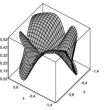
Figure 1: The figure shows two surfaces given by the fidelity $f$ of $\rho^{4}(x,y,\sigma=0.2)$ and its maximal singlet fraction $\max\{f,g\}$. Since $f>g$ for most of the values of the parameters, it is only at the left and right side, where we see that the two surfaces differ. This region shrinks if we increase $\sigma$ and disappears.

We have done the last step numerically and chosen $x\equiv\nu_{2}\equiv\nu_{1}$ and $y\equiv\nu_{4}\equiv\nu_{3}$. In this way we have a product of two identical two-mode state $\rho^{(2)}(x,y,\sigma,\sigma)$ at hand as seen from (63). Using the notation $\rho^{4}(x,y,\sigma)$ for the state, we compare the fidelity $f$ with the maximal entangled fraction (68). The result is that $f\geq g$ for most of the parameter values, and in particular for higher fidelities.

7 Distillation from lattice Fermions

To get another example for our scheme let us have a look at Fermions propagating on an infinite, regular lattice. For simplicity, we will restrict our discussion to one dimension, but everything we will say in this section, can be easily generalized to higher dimensions.

The system we are looking at has infinite degrees of freedom. Therefore the description used up to now has to be modified a bit (cf [3, 2] for a detailed exposition). As a starting point consider the Hilbert space $\mathcal{K}^{(\infty)}$ and the complex conjugation $J$ given by

$$\mathcal{K}^{(\infty)}=\mathrm{l}^{2}(\mathbb{Z})\oplus\mathrm{l}^{2}(\mathbb{Z})\ \text{and}\ J(x,y)=(\overline{y},\overline{x}).$$ (70)

Now we can consider as before Majorana operators $B(x)$ smeared by elements $x\in\mathcal{K}^{(\infty)}$, operating irreducibly on a (now infinite dimensional, but separable) Hilbert space $\mathcal{H}^{(\infty)}$ and satisfying the CAR. As in finite dimensions, a normalized element $\Omega_{S}\in\mathcal{H}^{(\infty)}$ describes a pure, quasifree state if its correlation functions are given in terms of Wick’s Theorem (cf. Equation (8)) and a basis projection $S\in\mathcal{B}(\mathcal{K}^{(\infty)})$, which is defined as in the finite dimensional case. The Hilbert space $\mathcal{H}^{(\infty)}$ and the operators $B(x)$ can be constructed as in Appendix A in terms of Fock spaces and creation/annihilation operators, but this is not important for us, because the triple consisting of $\mathcal{K}^{(\infty)}$, $J$ and $S$ fixes $\mathcal{H}^{(\infty)}$ and the $B(x)$ uniquely up to unitary equivalence.

Consider now a finite set $\Lambda$ of integers with cardinality $n$ and define the projection $I_{\Lambda}\in\mathcal{B}(\mathcal{K}^{(\infty)})$

$$(I_{\Lambda}x)_{j}=\chi_{\Lambda}(j)x_{j},\quad j\in\mathbb{Z}$$ (71)

where $\chi_{\Lambda}$ denotes the characteristic function of $\Lambda$. This projection commutes with $J$ (i.e. it is a real projection) and defines therefore a (finite dimensional) subsystem of the infinitely extended system. It is completely described by the algebra

$$\mathcal{A}_{\Lambda}=\operatorname{span}\{B(x_{1})\cdots B(x_{l})\,|\,l\in\mathbb{N},\ I_{\Lambda}x_{j}=x_{j}\forall j=1,\dots,l\}$$ (72)

which is isomorphic to the CAR algebra of $n$ modes. All operations, measurements, etc., which only affect the modes located in $\Lambda$ (and leave the rest of the system untouched) can be described in terms of this algebra. It is acting reducibly on $\mathcal{H}^{(\infty)}$, but we can cure this defect with a twisted tensor product. In analogy to (17) we can introduce a unitary

$$U_{\Lambda}:\mathcal{H}^{(\infty)}\rightarrow\mathcal{H}^{(n)}\otimes\mathcal{H}^{(\infty)}$$ (73)

such that

$$U_{\Lambda}B(x)U_{\Lambda}^{*}=\begin{cases}B(x)\otimes{\leavevmode{\rm 1\mkern-4.8muI}}&x\in I_{\Lambda}\mathcal{K}^{(\infty)}\cong\mathcal{K}^{(n)}\\ \theta\otimes B(x)&x\in({\leavevmode{\rm 1\mkern-4.8muI}}-I_{\Lambda})\mathcal{K}^{(\infty)}\cong\mathcal{K}^{(\infty)},\end{cases}$$ (74)

where $\mathcal{H}^{(n)}$ denotes, as before, the Fermionic Fockspace of $n$ modes. Dropping the complementary subsystem (which is now infinite dimensional) can be described again by the channel (cf. Equation (18)

$$\mathcal{B}(\mathcal{H}^{(n)})\ni A\mapsto\Delta_{\Lambda}(A)=U_{\Lambda}^{*}A\otimes{\leavevmode{\rm 1\mkern-4.8muI}}U_{\Lambda}\in\mathcal{B}(\mathcal{H}^{(\infty)}).$$ (75)

After applying this operation, the remaining $n$ modes are in the quasifree state $\rho_{S,\Lambda}$ with covariance matrix $S_{\Lambda}=I_{\Lambda}SI_{\Lambda}$ and we end up with the structure studied in Section 2.

Now let us come back to distillation and assume that Alice and Bob share an infinite 1-dimensional lattice containing a number (typically infinite) of Fermions. They can control only two contiguous regions $\Lambda_{A}$ and $\Lambda_{B}$ of $L$ lattice sites each and located at a distance of $N$ sites. Everything outside of $\Lambda=\Lambda_{A}\cup\Lambda_{B}$ can not be manipulated and is therefore ignored. In other words we apply the channel $\Delta_{\Lambda}$ defined in Equation (75) and get a bipartite Fermionic system consisting of $2L$ modes where the projections $I_{\Lambda_{A}}$ and $I_{\Lambda_{B}}$ play the role of $I_{A}$ and $I_{B}$ from Section 3. Hence we can apply the optimal protocol studied in Section 5 and calculate the success probability $p(L,N)$ and the fidelity $f(L,N)$ of the output systems. Both quantities depend on the geometry of the regions $\Lambda_{A}$ and $\Lambda_{B}$ (i.e. their length $L$ and distance $N$) and to study this functional behavior gives a deep insight how distillable entanglement is distributed along the chain.

Particularly interesting is the question, whether $p$ and $f$ can be made (as a function of $L$) arbitrarily close to 1. This would imply that using a sufficiently big chunk of the system is as good as using a sufficiently large number of the same system in the same state (which is typically done in ordinary distillation protocols such as hashing, and we have assumed this in Section 4, too). In this sense our result is closely related to the question how much entanglement can be distilled with certainty from one copy of an infinitely extended system. This is called the systems one copy entanglement and studied in a number of papers [14, 8, 13].

8 Free Fermions hopping on a 1-dimensional lattice

As an explicit example for the discussion from the last section let us consider the unique ground state of free Fermions hopping on a infinite, 1-dimensional, regular lattice (i.e. $\mathbb{Z}$). It is given by

$$S=\mathcal{F}^{-1}\left(\begin{array}[]{cc}E&0\\ 0&1-E\end{array}\right)\mathcal{F}$$ (76)

where

$$\mathcal{K}^{(\infty)}\ni F\mapsto\mathcal{F}(F)\in\operatorname{L}^{2}(S^{1})\otimes\mathbb{C}^{2},\quad\mathcal{F}(F)(x)=\frac{1}{\sqrt{2\pi}}\sum_{j=-\infty}^{\infty}e^{inx}F_{n}$$ (77)

is the Fourier transform and $E\in\mathcal{B}(\operatorname{L}^{2}(S^{1}))$ the projection to the upper half-circle. Proofs and further references for all of this can be found in [4].

As in the last section we will restrict the state to the region $\Lambda$ with

$$\Lambda_{A}=[-L,0),\quad\Lambda_{B}=[N,N+L),\quad\Lambda=\Lambda_{A}\cup\Lambda_{B}.$$ (78)

This results in the restricted density matrix $\rho_{I_{\Lambda}SI_{\Lambda}}$, with a covariance matrix $I_{\Lambda}SI_{\Lambda}$ which becomes in an appropriately chosen real basis

$$I_{\Lambda}SI_{\Lambda}=\left(\begin{array}[]{cc}{\leavevmode{\rm 1\mkern-4.8muI}}_{A}/2+iX&iY\\ -iY^{T}&{\leavevmode{\rm 1\mkern-4.8muI}}_{B}/2+iZ\end{array}\right)$$ (79)

with

$$X=Z=\left(\begin{array}[]{cc}0&iF_{0}\\ -iF_{0}&0\end{array}\right),\quad Y=\left(\begin{array}[]{cc}0&iF_{N+L}\\ -iF_{N+L}&0\end{array}\right)$$ (80)

and the $L\times L$ matrix $F_{r}$ ($r=0,N$) is given by

$$(F_{r})_{jk}=\begin{cases}0&\text{if}\ j=k+r\\ \frac{\sin\left(\frac{(j-k+r)\pi}{2}\right)}{(j-k+r)\pi}&\text{otherwise.}\end{cases}$$ (81)

Our goal is now to consider the distillation of qubit pairs from bipartite systems in such a state. The crucial step on the algorithmic side is to determine the subsystem projection $\hat{D}$ and the partial isometry $\hat{V}$ from $I_{\Lambda}SI_{\Lambda}$. This is done in terms of the singular value decomposition

$$Y=\sum_{j=1}^{2L}\lambda_{j}|\phi_{j}\rangle\langle\Phi_{j}|,\quad\lambda_{1}\geq\lambda_{2}\geq\dots\lambda_{2L}$$ (82)

of the matrix $Y$ from Equation (80). This gives rise to

$$\hat{D}_{A}=\sum_{j=1}^{4}|\phi_{j}\rangle\langle\phi_{j}|,\quad\hat{D}_{B}=\sum_{j=1}^{4}|\Phi_{j}\rangle\langle\Phi_{j}|,\quad\hat{V}=\sum_{j=1}^{4}|\phi_{j}\rangle\langle\Phi_{j}|.$$ (83)

All other quantities (in particular the probability $p$ and the fidelity $f$) can be derived from these three matrices (cf. Theorem 4.1 and 4.2).

Unfortunately, even for the matrices $F_{0},F_{N+L}$ with their very regular structure the singular value problem is not explicitly solvable. They are, however, Toeplitz matrices and we can at least provide an algorithm to derive $D_{\Lambda}SD_{\Lambda}$ which is quite efficient (in time and space) and which allows to do numerical calculations (at least) in the range $L=10^{4}-10^{6}$. One possible strategy (and the one we have used) is to use iterative procedures like the Lánczos method, which only needs matrix-vector multiplications. The latter can then be implemented by embedding the Toeplitz matrix $T$ into a bigger circulant matrix $C$ and to calculate the product $Cx$ for a column vector $x$ by a discrete Fourier transform. The product $Ty$ can then be calculated by first padding $y$ with zeros to fit the size of $C$ (which results in a higher dimensional vector $x$) and projecting out at the end the relevant dimensions from $Cx$.

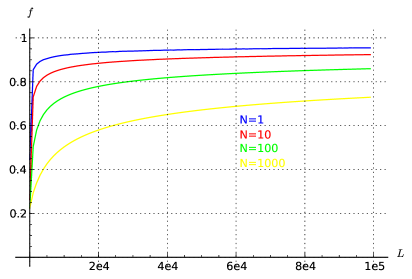
Figure 2: Plot of the entanglement fidelity $f$ as a function of the block length $L$ for fixed block distances $N=0,10,100,1000$.

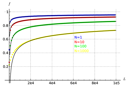
Figure 3: Entanglement fidelity $f(L)$ for $N=1,10,100,1000$ fitted with a model function (black curves) of the type $1-b/L^{a}$.

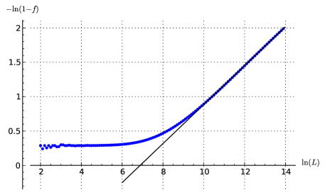
Figure 4: $-\log(1-f)$ as a function of $\log(L)$ for $N=1000$. For large $L$ the functional behavior seems to be linear (cf. the black curve).

Let us discuss now the result of our analysis. Figures 2 and 3 show $f$ as a function of $L$ for fixed block distances $N=1,10,100,1000$. In Figure 3 we have fitted the data with a model function of the form

$$f(L,N)=1-\frac{b(N)}{L^{a(N)}}.$$ (84)

It is easy to see that for small values of the block length $L$ this fit is not very good (in particular for larger block distance $N$). Therefore we have used only data $(L,f(N,L))$ with $L\geq 20000$ for calculating the fit parameters $a$ and $b$ (using a least square fit). This difference between the behavior for small and large $L$ becomes much clearer in Figure 4 where we have plotted $-\log(1-f)$ against $\log(L)$. The linear part for bigger values of $\log(L)$ correspond to the $1-b/L^{a}$ behavior in Figure 3.

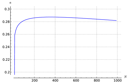
Figure 5: Fit parameter $a$ as a function of $N$. The black curve represents the average of the values for $N\geq 400$.

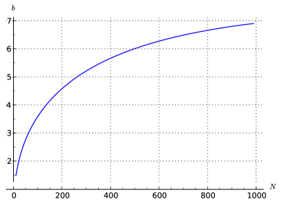
Figure 6: Fit parameter $b$ as a function $N$. For $N>500$ the data is fitted logarithmically.

To get an idea how the two fit parameter $a$ and $b$ depend on $N$ we have made a least square fit for the data $(L,f(L,N))$ with $L=10+1000k$, $k\in[20,100)$ and for all $N=0+10n$ with $n\in[0,100)$. The results are shown in Figures 5 and 6. We can see that for larger values of $N$ the parameter $a$ is almost constant, while $b$ seems to grow sub-linearly. Note that it is dangerous to say more at this point, because small fluctuations can be a consequence of the fitting algorithm rather than a real physical effect.

More insight we can get from a look on the function $L(N,x)$ which provides the minimal length of the intervals $\Lambda_{A/B}$ we need to get $f(L(N,x),N)\geq x$. The result is shown in Figure 7. We can see that the behavior looks linear and close inspection of the numerical data indeed shows that at least for large values of $N$ the behavior is as linear as it can be for a function which only takes integer values.

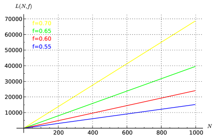
Figure 7: Minimal interval length $L(N,x)$ needed to get a fidelity $f\geq x$ if the distance is $N$.

Another important function we can investigate is the probability $p$ to get during a joint parity measurement on the restricted system in the state $\rho_{D_{\Lambda}SD_{\Lambda}}$ the results $++$ or $--$.

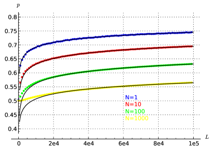
Figure 8: Probability $p(L,N)$ for $N=1,10,100,1000$ fitted with a model function (black curves) of the type $1-b/L^{a}$.

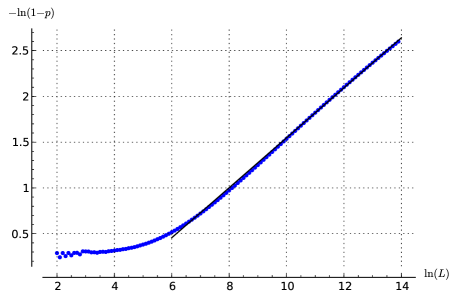
Figure 9: $-\log(1-p)$ as a function of $\log(L)$ for $N=1000$. For large $L$ the functional behavior is linearly approximated.

In Figure 8 we can see that the behavior of $p$ as a function of $L$ looks quite similar as $f(L)$ from Figure 3. Again we can find a good fit for larger $L$ with a function of the type $1-a/L^{b}$. This is also confirmed by Figure 9 where we have again plotted $-\log(1-p)$ as function of $\log(p)$. The behavior of $p$ for small $L$ and $N$ seems, however, to be more irregular than the one for $f$ and if we look very closely at Figure 9 we can see that the linear fit is not as good as in Figure 4 (the blue curve is bending a little bit around the black line).

9 Conclusions

We have presented a distillation scheme which can be applied to a bipartite Fermionic system in a generic quasifree state, and while it is in general not optimal we have found substantial evidence that we do not waste too much entanglement originally hidden in the given state. The asymptotic rate of this protocol (or equivalently the entanglement fidelity of the isotropic states we get at an intermediate step) can be calculated explicitly and can therefore be used as tool to analyze entanglement of Fermionic systems.

The latter is particularly true for lattice Fermions. The analysis of the previous section showed that a numerical study is possible for effectively very large systems up to $10^{6}$ lattice sites. We have only studied a very special quasifree state here, but the algorithms used can be easily generalized to other translation invariant quasifree states: Their covariance operator is a ($2\times 2$-matrix valued) multiplication operator and the matrix $I_{\Lambda}SI_{\Lambda}$ of the restricted state (which can be easily calculated by Fourier integrals) is again a (block-)Toeplitz operator.

The results about free Fermions on a lattice, derived in the last section are interesting in their own right and indicate some structure in the fidelity $f(N,L)$ and the block length $L(N,f)$. Note that the latter is closely related to a quantity proposed in [13] to analyze states with infinite one-copy entanglement. The numerical study presented so far does not tell us the whole story of course, but it gives us some hints what we might expect from a more detailed, analytic study. The latter is of course difficult but a deeper discussion of the asymptotic behavior of $f$ and $L$ (which is related to the asymptotic behavior of the singular value decomposition of the off-diagonal blocks $Y$) seems to be a realistic goal.

Appendix A The self-dual formalism

The purpose of this appendix to connect the self-dual formalism presented in Section 2 to the more familiar description in terms of creation and annihilation operators $c_{j},c_{j}^{*}$, $j=1,\dots,n$ operating on Fermionic Fockspace $\mathcal{H}^{(n)}=\mathcal{F}_{-}(\mathbb{C}^{n})$. They satisfy the canonical anticommutation relations (CAR)

$$\{c_{j},c_{k}\}=\{c_{j}^{*},c_{k}^{*}\}=0,\quad\{c_{j},c_{k}^{*}\}=\delta_{jk}{\leavevmode{\rm 1\mkern-4.8muI}}$$ (85)

and they are irreducible, i.e. for any operator $A$ on $\mathcal{H}^{(n)}$ we have

$$[A,c_{j}]=[A,c_{k}^{*}]=0\ \forall j,k=1,\dots,n\Rightarrow A=\lambda{\leavevmode{\rm 1\mkern-4.8muI}}$$ (86)

for some $\lambda\in\mathbb{C}$. The latter implies in particular that the *-algebra generated by the $c_{j},c_{k}^{*}$ coincides with $\mathcal{B}(\mathcal{H}^{(n)})$.

Alternatively we can introduce the Majorana operators

$$B_{a}=\begin{cases}\frac{1}{\sqrt{2}}(c_{a}+c_{a}^{*})&\text{if $a=1,\dots,n$}\\ \frac{i}{\sqrt{2}}(c_{a-n}-c_{a-n}^{*})&\text{if $a=n+1,\dots,2n$}.\end{cases}$$ (87)

The $B_{a}$ are selfadjoint and from (85) we immediately get

$$\{B_{a},B_{b}\}=\delta_{a,b}{\leavevmode{\rm 1\mkern-4.8muI}}.$$ (88)

Irreducibility of the $c_{j},c_{k}^{*}$ implies irrducibility of the $B_{a}$ and vice versa.

Finally we can smear the $B_{a}$ with a “test function” $x\in\mathbb{C}^{2n}$

$$B(x)=\sum_{a=1}^{2n}x_{a}B_{a},\quad x=(x_{a})_{a=1,\dots,2n}\in\mathcal{K}^{(n)}=\mathbb{C}^{2n}$$ (89)

to get the structure we have started with in Section 2. Note that in this case we have $\mathcal{K}^{(n)}=\mathbb{C}^{(2n)}$ and $J$ is given by complex conjugation in the canonical basis ($(Jx)_{a}=\bar{x}_{a}$). It is easy to see that the $B(x)$ are irreducible, linear in $x$ and satisfy the CAR in the form (4).

If we start with the smeared operators we can derive the $B_{a}$ by $B_{a}=B(e_{a})$ if $e_{a}$ denotes the canonical basis in $\mathcal{K}^{(n)}$. Instead of the $e_{a}$, however, we can use any real basis $\tilde{e}_{a},a=1,\dots,2n$ of $\mathcal{K}^{(n)}$ to get an irreducible family of selfadjoint operators $\tilde{B}_{a}=B(\tilde{e}_{a})$ on $\mathcal{H}^{(n)}$, which satisfy the CAR (88) and are therefore as good to describe the system as the orginal $B_{a}$. In other words: The smeared operators $B(x)$ provide a coordinate free description of the system, while the $B_{a}$ (and the corresponding $c_{j},c_{k}^{*}$) are coordinate dependent.

This distinction is not purely academic, because the $c_{j},c_{k}^{*}$ (and therefore the $B_{a}$ from which the $c_{j},c_{k}^{*}$ can be derived) are accompanied by a distinguished state: The Fock vacuum which is given by the condition $c_{k}^{*}\Omega=0$ $\forall k=1,\dots,n$. The smeared operators $B(x)$, however, does not prefer any state – we have to choose a real basis first.

To make the last statement more precise let us show how the definition of Fock states in Section 2 is related to the ordinary Fock vacuum. To this end let us consider a basis projection $E\in\mathcal{B}(\mathcal{K}^{(n)})$ and introduce orthonormal bases $(f_{j}^{(1)})_{j=1,\dots,n}$ and $(f_{k}^{(2)})_{k=1,\dots,n}$ in the range $\operatorname{Ran}E\subset\mathcal{K}^{(n)}$ and kernel $\ker E\subset\mathcal{K}^{(n)}$ of $E$ respectively. Obviously

$$e_{a}=\begin{cases}\frac{1}{\sqrt{2}}(f_{a}^{(1)}+f_{a}^{(2)})&\text{if $a=1,\dots,n$}\\ \frac{i}{\sqrt{2}}(f_{a-n}^{(1)}-f_{a-n}^{(2)})&\text{if $a=n+1,\dots,2n$}.\end{cases}$$ (90)

is a real basis and a short calculation shows that the vacuum state $\Omega\in\mathcal{H}^{(N)}$ given by

$$B_{a}=B(e_{a}),\quad c_{k}=\frac{1}{\sqrt{2}}(B_{k}+iB_{k+n}),\quad c_{k}^{*}\Omega=0\ \forall k=1,\dots,n$$ (91)

satisfies

$$\langle\Omega,B(x_{1})B(x_{2})\Omega\rangle=\langle Jx_{1},Ex_{2}\rangle.$$ (92)

Validity of the relations in (8) follows from Wick’s theorem. Therefore $\Omega\in\mathcal{H}^{(n)}$ is the Fock state with covariance operator $E$.

Appendix B The parity operator

In this appendix we will present a proof of Theorem 4.1 and Equation (13). Unless something else is explicitly stated we will use the notations from Section 2. The core result is the following proposition.

Proposition B.1

Let $e_{a}\in\mathcal{K}^{(n)}$, $a=1,\dots,2n$ be a real basis of the reference space $\mathcal{K}^{(n)}$ and define

$$\theta=2^{n}i^{n}B(e_{1})\dots B(e_{2n});$$ (93)

then the following statements hold:

1. $\theta$ is a selfadjoint unitary.

2. $\theta$ implements the parity automorphism $\Theta$, i.e. $\theta B(x)\theta=-B(x)$ for all $x\in\mathcal{K}^{(n)}$.

3. For each unitary $R\in\mathcal{B}(\mathcal{K}^{(n)})$ commuting with $J$ (i.e. each real orthogonal transformation of ($\mathcal{K}^{(n)}$,$J$)) we have

   $$\theta=\det(R)i^{n}2^{n}B(Re_{1})\dots B(Re_{2n}).$$ (94)

Proof.  Item 1. $\theta$ is unitary: Due to $B(h)^{*}=B(Jh)$ and $Je_{a}=e_{a}$ all the operators $B_{a}$ are selfadjoint, hence

$$\theta^{*}=2^{n}(-i)^{n}B(e_{2n})\cdots B(e_{1})$$ (95)

and this implies together with $\{B(e_{a}),B(e_{a})\}=2B(e_{a})^{2}={\leavevmode{\rm 1\mkern-4.8muI}}$ that $\theta\theta^{*}=\theta^{*}\theta={\leavevmode{\rm 1\mkern-4.8muI}}$.

To see that $\theta$ is also selfadjoint, note first that $B(e_{a})$ and $B(e_{b})$ anticommute iff $a\neq b$. Now reverse inductively the ordering of the factors in Equation (95). The first two steps lead to

$$\theta=-i^{n}2^{n}B(e_{1})B(e_{2d})\cdots B(e_{2})=-i^{n}2^{n}B(e_{1})B(e_{2})B(e_{2n})\cdots B(e_{3})=\dots\ .$$ (96)

Hence we pick up an additional factor $-1$ at each second step (i.e. while moving a $B(e_{a})$ with $a$ odd to the $a^{\mathrm{th}}$ position). In this way we get in total a factor $(-1)^{n}$, which shows with Equation (95) that $\theta$ is selfadjoint as stated.

Item 2. With a similar argument we can show that for all $a=1,\dots,2n$ we have

$$\theta B(e_{a})=(-1)^{2n-1}B(e_{a})\theta=-B(e_{a})\theta.$$ (97)

As a selfadjoint unitary $\theta$ satisfies $\theta^{2}={\leavevmode{\rm 1\mkern-4.8muI}}$. This implies $\theta B(e_{a})\theta=-B(e_{a})$, which completes the proof of item 2.

Item 3. If $R$ is real orthogonal, the basis $\tilde{e}_{a}=Re_{a}$ is again a real basis and the reasoning from above applies. Hence

$$\theta_{R}=i^{n}2^{n}B(Re_{1})\dots B(Re_{2n})$$ (98)

is a selfadjoint unitary and implements the parity automorphism $\Theta$. Only the operators $\pm\theta$ have these properties, and therefore we only have to check the sign. To this end consider a quasifree state $\rho_{S}$ with covariance matrix $S$. To complete the proof we have to show that $\operatorname{tr}(\rho_{S}\theta_{R})=\det(R)\operatorname{tr}(\rho_{S}\theta)$.

According to the properties of the covariance operator $S$, we can introduce a real, antisymmetric matrix $\tilde{S}$ by

$$i\tilde{S}_{ab}=\langle e_{a},(S-{\leavevmode{\rm 1\mkern-4.8muI}}/2))e_{b}\rangle.$$ (99)

With the definition of quasifree states we therefore get

$$\operatorname{tr}(\rho_{S}\theta) =2^{n}i^{n}\operatorname{tr}(\rho_{S}B(e_{1})\cdots B(e_{2n}))$$ (100)

$$=2^{n}i^{n}\sum\operatorname{sign}(p)\prod_{j=1}^{n}\langle e_{p(2j-1)},Se_{p(2j)}\rangle,$$ (101)

$$=2^{n}i^{n}\operatorname{sign}(p)\prod_{j=1}^{n}i\tilde{S}_{p(2j-1),p(2j)}$$ (102)

$$=2^{n}(-1)^{n}\operatorname{Pf}(\tilde{S})$$ (103)

and similarly

$$\operatorname{tr}(\rho_{S}\theta_{R})=2^{n}(-1)^{n}\operatorname{Pf}(R^{*}\tilde{S}R)$$ (104)

where we have identified in abuse of notation $R$ with its matrix representation in the basis $e_{a}$. The statement now follows from the properties of Pfaffian (i.e. $\operatorname{Pf}(R^{*}\tilde{S}R)=\det(R)\operatorname{Pf}(\tilde{S})$). $\Box$

Note that we have shown in addition that the expectation value of $\theta$ in a quasifree state $\rho_{S}$, is given by

$$\operatorname{tr}(\rho_{S}\theta)=2^{n}(-1)^{n}\operatorname{Pf}(\tilde{S}).$$ (105)

This is very useful in the proof of Theorem 4.1. The only problem is that we have decided about the sign of $\theta$ in an arbitrary way. This can be fixed with the following Lemma, which uses the notations introduced in Section 3.

Lemma B.2

Consider a bipartite, Fermionic system consisting of $2m$ modes, and a quasifree, maximally entangled state $\psi_{E}$ with covariance matrix $E\in\mathcal{B}(\mathcal{K}^{(2m)})$.

1. There is a real basis $e_{a}\in\mathcal{K}^{(2m)}$, $a=1,\dots,4m$ such that

   $$e_{1},\dots,e_{2m}\in\mathcal{K}_{A}^{(m)},\quad e_{2m+1},\dots,e_{4m}\in\mathcal{K}_{B}^{(m)}$$ (106)

   and

   $$Y_{E}e_{2m+j}=e_{2m}\quad\forall j=1,\dots,2m$$ (107)

   holds, where $Y_{E}=-iI_{A}EI_{B}$ as in Equation (24).

If $\theta$ denotes the parity operator given by Equation (94) and this basis, we get

$$\langle\psi_{E},\theta\psi_{E}\rangle=(-1)^{m}.$$ (108)

Proof.  Since $\psi_{E}$ is maximally entangled by assumption, the off-diagonal operator $Y$ is a partial isometry. Hence we can construct the basis $e_{a}$ by choosing $e_{2m+1},\dots,e_{4m}$ as an arbitrary real basis of $\mathcal{K}_{B}^{(m)}$ and defining $e_{1},\dots,e_{2m}$ by (107). In this basis $E$ becomes

$$E=\frac{1}{2}\left(\begin{array}[]{cc}{\leavevmode{\rm 1\mkern-4.8muI}}&i{\leavevmode{\rm 1\mkern-4.8muI}}\\ -i{\leavevmode{\rm 1\mkern-4.8muI}}&{\leavevmode{\rm 1\mkern-4.8muI}}.\end{array}\right)$$ (109)

Inserting this into (105) we get

$$\langle\psi_{E},\theta\psi_{E}\rangle=2^{2m}\operatorname{Pf}(\tilde{E})$$ (110)

with

$$\tilde{E}=\frac{1}{2}\left(\begin{array}[]{cc}0&{\leavevmode{\rm 1\mkern-4.8muI}}\\ -{\leavevmode{\rm 1\mkern-4.8muI}}&0\end{array}\right).$$ (111)

The Pfaffian of $\tilde{E}$ is easy to calculate and gives $(-1)^{m(2m-1)}2^{-2m}=(-1)^{m}2^{-2m}$. Inserting this in (110) we get the result. $\Box$

Proof of Theorem 4.1. Since $P_{+}=({\leavevmode{\rm 1\mkern-4.8muI}}+\theta)/2$ holds, the probability $p=\operatorname{tr}(\rho_{S}P_{+})$ can be calculated as $p=(1+\operatorname{tr}(\rho_{S}\theta))/2$ where the sign of the parity is chosen by $\langle\psi_{E},\theta\psi_{E}\rangle=1$. Hence the statement follows from Equation (105) and Lemma B.2. $\Box$.

Appendix C The optimality proof

The purpose of this appendix is to provide the proof of the optimality Theorem 5.1. The crucial assumption is that the diagonal subblocks of the covariance operator $S$ satisfy $X=0$ or $Z=0$. In both cases the quantity $pf$ we have to optimize becomes (this follows directly from Equation (46), and properties of the Pfaffian and the determinant):

$$pf(S,m,D,V)=\frac{1}{2^{2m}}\left(\left|\det(D_{A}YD_{B}+V)\right|+\left|\det(D_{A}YD_{B}-V)\right|\right).$$ (112)

Here we have identified in abuse of notation the spaces $D_{A}\mathcal{K}^{(2m)}$ and $D_{B}\mathcal{K}^{(2m)}$ and interpreted the operators $D_{A}YD_{B}\pm V$ as operators on $D_{A}\mathcal{K}^{(2m)}$, such that the determinants have a chance to lead to a non-zero value. The first step in the proof is to optimize with keeping $D$ fixed.

Proposition C.1

Consider a bipartite Fermionic system consisting of $2m$ modes and a quasifree state $\rho_{S}$ with covariance matrix $S$ satisfying $X_{S}=0$ or $Z_{S}=0$. Assume in addition that the off-diagonal block has maximal rank $2m$, then we have

$$pf(S,m,{\leavevmode{\rm 1\mkern-4.8muI}},V)\leq pf(S,m,{\leavevmode{\rm 1\mkern-4.8muI}},\hat{V})=\prod_{k=1}^{2m}\frac{1+\lambda_{k}}{2}+\prod_{k=1}^{2m}\frac{1-\lambda_{k}}{2}$$ (113)

where $\lambda_{k}$ denotes the eigenvalues of $|Y|$ and $\hat{V}$ is the partial isometry defined in Equation (52).

Proof.  Let us choose a real basis $e_{a}$ in $\mathcal{K}^{(2m)}$ such that $Y$ is diagonalized, i.e. $\langle e_{j},Ye_{k+2m}\rangle=\delta_{jk}\lambda_{k}$. The matrix elements $V_{jk}=\langle e_{j},Ve_{k+2m}\rangle$ of $V$ in the same basis form a orthogonal matrix. Hence the determinants in Equation (112) become

$$\det(Y\pm V)=\sum_{p}\epsilon_{p}\prod_{j=1}^{2m}(V_{jp(j)}\pm\delta_{jp(j)}\lambda_{j}),$$ (114)

where the sum is taken over all permutations of $1,\dots,2m$. This can be rewritten as a polynomial in the $\lambda_{j}$:

$$\det(Y+V)=\sum_{\Sigma\subset\{1,\dots,2m\}}\prod_{j\in\Sigma}\lambda_{j}\det(V_{\Sigma}).$$ (115)

$V_{\Sigma}$ denotes the matrix we get from $V$ if we remove the $j^{\mathrm{th}}$ row and column for all $j\in\Sigma$. Now assume that both determinants have the same sign. Then Equation (112) leads to

$$pf(S,m,{\leavevmode{\rm 1\mkern-4.8muI}},V)=2\sum_{\begin{subarray}{c}\Sigma\subset\{1,\dots,2m\}\\ \Sigma\ \text{even}\end{subarray}}\prod_{j\in\Sigma}\lambda_{j}\det(V_{\Sigma}).$$ (116)

Now note that $0<\lambda_{j}\leq 1$ for all $j$ and $V_{\Sigma}$ is a submatrix of an orthogonal matrix. Hence $|\det V_{\Sigma}|\leq 1$ with equality iff $V_{\Sigma}$ is orthogonal again. The expression in (116) is maximal iff $\det V_{\Sigma}=1$ for all $\Sigma$. But this is implies that all submatrix $V_{\Sigma}$ are orthogonal. This is only possible if $V$ is diagonal. A similar reasoning holds if both determinants in (112) have opposite signs (instead of (116) we get a sum over subsets with an odd cardinality).

This shows that $Y$ has to be diagonal with eigenvalues $\pm 1$. The optimal value of $pf(S,m,{\leavevmode{\rm 1\mkern-4.8muI}},V)$ then becomes

$$\mathrm{fid}(\Gamma_{+},\Gamma_{-})+\mathrm{fid}(\Gamma_{-},\Gamma_{+})$$ (117)

with

$$\mathrm{fid}(\Gamma_{+},\Gamma_{-})=\left|\prod_{j\in\Gamma_{+}}(1+\lambda_{j})\prod_{k\in\Gamma_{-}}(-1+\lambda_{k})\right|=\prod_{j\in\Gamma_{+}}(1+\lambda_{j})\prod_{k\in\Gamma_{-}}(1-\lambda_{k})$$ (118)

where $\Gamma_{+}$ and $\Gamma_{-}$ are disjoint sets of integers satisfying $\Gamma_{+}\cup\Gamma_{-}=\{1,\dots,2m\}$. Also note that the second equation in (118) holds, due to $0<\lambda_{j}\leq 1$. The proposition is proved if we can show that

$$\mathrm{fid}(\{1,\dots,2m\},\emptyset)+\mathrm{fid}(\emptyset,\{1,\dots,2m\})\geq\mathrm{fid}(\Gamma_{+},\Gamma_{-})+\mathrm{fid}(\Gamma_{-},\Gamma_{+})$$ (119)

holds. To prove this inequality rewrite $\mathrm{fid}$ as

$$\mathrm{fid}(\Gamma_{+},\Gamma_{-}) =\mathrm{fid}(\Gamma_{+},\emptyset)\sum_{\gamma\subset\Gamma_{-}}(-1)^{|\gamma|}\prod_{j\in\gamma}\lambda_{j}$$ (120)

$$=\mathrm{fid}(\emptyset,\Gamma_{-})\sum_{\gamma\subset\Gamma_{+}}\prod_{j\in\gamma}\lambda_{j}.$$ (121)

This leads to

$$\mathrm{fid}(\Gamma_{+},\Gamma_{-})+\mathrm{fid}(\Gamma_{-},\Gamma_{+})=\sum_{\gamma\subset\Gamma_{-}}\bigl{(}(-1)^{|\gamma|}\mathrm{fid}(\Gamma_{+},\emptyset)+\mathrm{fid}(\emptyset,\Gamma_{+})\bigr{)}\prod_{j\in\gamma}\lambda_{j}.$$ (122)

The definition of $\mathrm{fid}$ shows that

$$\mathrm{fid}(\Gamma_{+},\emptyset)\geq\mathrm{fid}(\emptyset,\Gamma_{+})$$ (123)

holds. Hence each summand in (122) belonging to $\gamma$ with odd cardinality is negative. In contrast to that we get

$$\mathrm{fid}(\{1,\dots,2m\},\emptyset)+\mathrm{fid}(\emptyset,\{1,\dots,2m\})=\sum_{\gamma\subset\Gamma_{-}}\bigl{(}\mathrm{fid}(\Gamma_{+},\emptyset)+(-1)^{|\gamma|}\mathrm{fid}(\emptyset,\Gamma_{+})\bigr{)}\prod_{j\in\gamma}\lambda_{j}$$ (124)

where all summands are positive. This completes the proof. $\Box$

Proof of Theorem 5.1. We are now ready to complete the proof of Theorem 5.1. Hence let us consider $2L$ modes in the quasifree $\rho_{S}$, an integer $m<L$ and a real projection $D=D_{A}\oplus D_{B}\in\mathcal{K}^{(2m)}$. If $V_{DSD}$ denotes the partial isometry given by the polar decomposition of $D_{A}YD_{B}$, we get with Proposition C.1:

$$pf(S,m,D,V_{DSD})=\frac{1}{2^{2m}}\prod_{k=1}^{2m}\frac{1+\tilde{\lambda}_{k}}{2}+\prod_{k=1}^{2m}\frac{1-\tilde{\lambda}_{k}}{2}=\frac{1}{2^{2m}}\sum_{\begin{subarray}{c}\Sigma\subset\{1,\dots,2m\}\\ |\Sigma|\ \text{even}\end{subarray}}\prod_{j\in\Sigma}\tilde{\lambda}_{j}$$ (125)

where $\tilde{\lambda}_{j}$ are the eigenvalues of $|Y_{DSD}|$ given in decreasing order. Obviously this quantity is optimized, if the $\tilde{\lambda}_{j}$ are as big as possible. Hence the theorem is proved if we can show that each $D$ satisfies

$$\lambda_{j}\geq\tilde{\lambda}_{j}\quad\forall j=1,\dots,2m$$ (126)

with equality only if $D=\hat{D}$. Here $\lambda_{1},\dots,\lambda_{2L}$ are the eigenvalues of $|Y|$.

To get this bound note first that instead of $|Y|$ and $|Y_{DSD}|$ we can look at the eigenvalues of $Y^{*}Y$ and $Y_{DSD}^{*}Y_{DSD}$. To get the corresponding bound we will use the Courant-Fischer theorem (Theorem 4.2.11 of [10]) which states that the $k^{\mathrm{th}}$ highest eigenvalue $\lambda_{k}$ of a hermitian matrix $A$ is given by

$$\lambda_{k}=\sup_{F}\inf_{\begin{subarray}{c}x\neq 0\\ Fx=0\end{subarray}}\frac{\langle x,Ax\rangle}{\langle x,x\rangle}$$ (127)

where the supremum is taken over all rank $k-1$ projections $F$. Now we get

$$\frac{\langle x,Y^{*}Yx\rangle}{\langle x,x\rangle} \geq\frac{\langle D_{B}x,Y^{*}YD_{B}x\rangle}{\langle x,x\rangle}$$ (128)

$$\geq\frac{\langle x,D_{B}Y^{*}D_{A}YD_{B}x\rangle}{\langle x,x\rangle}+\frac{\langle x,D_{B}Y^{*}({\leavevmode{\rm 1\mkern-4.8muI}}-D_{A})YD_{B}x\rangle}{\langle x,x\rangle}$$ (129)

$$\geq\frac{\langle x,D_{B}Y^{*}D_{A}YD_{B}x\rangle}{\langle x,x\rangle},$$ (130)

where we have used the fact that ${\leavevmode{\rm 1\mkern-4.8muI}}-D_{A}$ is a positive operator. This leads to

$$\sup_{F}\inf_{\begin{subarray}{c}x\neq 0\\ Fx=0\end{subarray}}\frac{\langle x,Y^{*}Yx\rangle}{\langle x,x\rangle}\geq\sup_{F}\inf_{\begin{subarray}{c}x\neq 0\\ Fx=0\end{subarray}}\frac{\langle x,D_{B}Y^{*}D_{A}YD_{B}x\rangle}{\langle x,x\rangle}.$$ (131)

Hence the $k^{\mathrm{th}}$ highest eigenvalue of $Y^{*}Y$ is greater or equal to the $k^{\mathrm{th}}$ highest eigenvalue of $D_{B}Y^{*}D_{A}YD_{B}$. Since this bound is attained by $\hat{D}=\hat{D}_{A}\oplus\hat{D}_{B}$ the theorem is proved. $\Box$

Proof of Corollary 5.2. We show that increasing $m$ by two decreases $pf$, i.e.

$$pf(S,m,\hat{D},\hat{V})\geq pf(S,m+2,\hat{D},\hat{V}).$$ (132)

To this end let us introduce first the polynomial

$$g=\frac{1}{2^{2m}}\sum_{\begin{subarray}{c}\Sigma\subset\{1,\dots,2m\}\\ |\Sigma|\ \text{odd}\end{subarray}}\prod_{j\in\Sigma}\lambda_{j}=\prod_{j=1}^{2m}\frac{1+\lambda_{j}}{2}-\prod_{j=1}^{2m}\frac{1-\lambda_{j}}{2}\leq pf(S,m,\hat{D},\hat{V})$$ (133)

Then we can express $pf(S,m+2,\hat{D},\hat{V})$ as

$$pf(S,m+2,\hat{D},\hat{V})=\frac{1}{4}(pf(S,m,\hat{D},\hat{V})+pf(S,m,\hat{D},\hat{V})\lambda_{m+1}\lambda_{m+2}+g\lambda_{m+1}+g\lambda_{m+2}).$$ (134)

The statement follows from Equation (133) and the fact that $\lambda_{m+1}\leq 1$ and $\lambda_{m+2}\leq 1$. $\Box$

References

- [1] L. Amico, R. Fazio, A. Osterloh and V. Vedral. Entanglement in many-body systems. Rev. Mod. Phys. 80, 517–576 (2008).
- [2] H. Araki. On quasifree states of and Bogoliubov automorphisms. Publ. Res. Inst. Math. Sci. 6, 385–442 (1970/71).
- [3] H. Araki. Bogoliubov automorphisms and Fock representations of canonical anticommutation relations. In Operator algebras and mathematical physics (Iowa City, Iowa, 1985), volume 62 of Contemp. Math., pages 23–41. Amer. Math. Soc., Providence, RI (1987).
- [4] H. Araki and T. Matsui. Ground states of the -model. Comm. Math. Phys. 101, no. 2, 213–245 (1985).
- [5] M.-C. Bañuls, J. I. Cirac and M. M. Wolf. Entanglement in Fermionic systems. Phys. Rev. A 76, 022311 (2007).
- [6] C. H. Bennett, D. P. DiVincenzo, J. A. Smolin and W. K. Wootters. Mixed-state entanglement and quantum error correction. Phys. Rev. A 54, no. 4, 3824–3851 (1996).
- [7] S. Bravyi. Lagrangian representation for fermionic linear optics. Quantum Inf. and Comp 5, no. 3, 216–238 (2005).
- [8] J. Eisert and M. Cramer. Single-copy entanglement in critical spin chains. Phys. Rev. A 72, 042112 (2005).
- [9] R. Haag. Local quantum physics. Springer, Berlin (1992).
- [10] R. A. Horn and C. R. Johnson. Matrix analysis. Cambridge University Press, Cambridge (1985).
- [11] J.-I. Cirac J. Schliemann, M. Kus, M. Lewenstein and D. Loss. Quantum correlations in two-fermion systems. Phys. Rev. A 64, 022303 (2001).
- [12] M. Keyl. Distilling entanglement from fermions. OSID 16, 243–258 (2009).
- [13] M. Keyl, T. Matsui, D. Schlingemann and R. F. Werner. Entanglement, Haag-duality and type properties of infinite quantum spin chains. Rev. Math. Phys. 18, no. 9, 935–970 (2006).
- [14] M. Keyl, D. Schlingemann and R. F. Werner. Infinitely entangled states. Quant. Inf. Comput. 3, no. 4, 281–306 (2003).
- [15] M. Keyl and D.-M. Schlingemann. The algebra of Grassmann canonical anticommutation relations and its applications to fermionic systems. J. Math. Phys. 51, no. 2, 023522 (2010).
- [16] E. Lieb, T. Schultz and M. Mattis. Two soluble models of an antiferromagnetic chain. Ann. Phys. (N.Y.) 16, 407–466 (1961).
- [17] H. Moriya. On separable states for composite systems of distingushable fermions. J. Phys. A 39, 3753–3762 (2006).
- [18] D. Schlingemann, M. Cozzini, M. Keyl and L. Campos Venuti. Maximally entangled fermions. Phys. Rev. A 78, 032301 (2008).
- [19] N. Schuch, F. Verstraete and J. I. Cirac. Quantum entanglement theory in the presence of superselection rules. Phys. Rev. A 70, 042310 (2004).
- [20] R. Verch and R. F. Werner. Distillability and positivity of partial transposes in general quantum field systems. Rev. Math. Phys. 17, no. 5, 545–576 (2005).
- [21] K. G. Vollbrecht and M. M. Wolf. Efficient distillation beyond qubits. Phys. Rev. A 67, 012303 (2003).