On the theory of magnetization in multiferroics: competition between ferro- and antiferromagnetic domains

Abstract

Many technological applications of multiferroics are based on their ability to reconstruct the domain structure (DS) under the action of small external fields. In the present paper we analyze the different scenarios of the DS behavior in a multiferroic that shows simultaneously ferro- and antiferromagnetic ordering on the different systems of magnetic ions. We consider the way to control a composition of the DS and macroscopic properties of the sample by an appropriate field treatment. We found out that sensitivity of the DS to the external magnetic field and the magnetic susceptibility in a low-field region are determined mainly by the destressing effects (that have magnetoelastic origin). In a particular case of Sr₂Cu₃O₄Cl₂ crystal we anticipate the peculiarities of the elastic and magnetoelastic properties at $T\approx 100$ K.

I Introduction

During the last ten years a special attention is paid to the materials in which magnetism coexists with the other types of ordering, i.e., ferroelectric Fert:2007 , elastic cruz:2006 , martensitic Chernenko:1995 . Solids that show strong coupling between the different types of ordering are often called multiferroics Ramesh:2007 . Growing interest to multiferroics is based on the possibility to i) control such macroscopic properties of a sample as conductivity, magnetization, elongation, with the suitable fields of different nature; ii) manipulate the state of the magnetically (electrically, etc.) inert materials (see, e.g., Refs. Chu:2007, ; desousa-2008-3, ).

One of the most technologically appealing property of multiferroics, namely, sensitivity of their macroscopic properties to the influence of small external fields is due to formation and reconstruction of the domain structure (DS) Fiebig:2002 . This adaptivity, ability to change macroscopic parameters (such as a shape, magnetization, electric polarization) in response to external forces is related with the finite size and boundary of the sample. While the physical mechanism of the DS formation is related with the sample boundary, reconstruction and restructurization of the domains under external fields depends upon the properties of the domain walls. If a potential barrier for the domains wall formation is high, switching between the different macroscopic states is sharp and field dependence of macroscopic parameters reveals a hysteresis. In the opposite case of low potential barrier, reconstruction of the DS takes place through the nucleation and growth of new domains and shows the features of liquid-like behavior: nonhysteretic transitions between the different macroscopic states, shape deformation, etc. The most interesting case on which we concentrate our attention in the present paper lies in-between: in multiferroics with the domains of different nature some types of the domains can easily nucleate and show soft-like behavior while the others could have high nucleation barrier and reveal themselves as solids.

The origin of the DS in the “single” ferroics, like ferromagnets (FM) and ferroelectrics, is well established Kittel:1949 and is attributed to the presence of long-range interactions between the magnetic or electric dipoles localized on different sites. The nonlocal character of the dipole forces ensures strong dependence of the equilibrium DS on the shape of the sample. In many important cases the DS of a single ferroic consists of the domains with opposite (sometimes noncollinear) directions of polarization and can be described thermodynamically on the basis of demagnetization energy.

Antiferromagnets (AFM) give an example of the more complicated materials with usually pronounced coupling between the magnetic order parameter and lattice strain. The behavior of equilibrium domain structure in AFM is very similar to the behavior of the DS in other ferroics with some “technical” distinctions: i) long-range dipole-dipole interactions responsible for the formation of equilibrium DS have a magnetoelastic origin and are described by the destressing gomonay:174439 (in contrast to depolarization or demagnetization) energy; ii) DS consists of the domains with different (nonparallel) orientations of AFM vectors.

Description of the DS in multiferroics seems to be much more complicated problem mostly due to the fact that the domains of different nature appear at different scales and thus form a hierarchical structure. Good example of such a complexity is given by FM martensites (see, e.g., Ref. Chernenko:1995, ) that are usually characterized by two independent order parameters lvov:1998 , magnetization and spontaneous strain. Cross-correlations between the magnetic and structural order parameters open a way to control a martensitic DS and, as a consequence, macroscopic deformation of a sample, with the external magnetic field (so-called giant magnetostriction Kokorin:1996(1) ).

Another example of multiferroic behavior is given by some of the high-temperature superconducting systems (like Sr₂Cu₃O₄Cl₂ or Ba₂Cu₃O₄Cl₂) that show simultaneously FM and AFM ordering on the different systems of copper ions. In contrast to FM martensites, the DS in these crystals is not hierarchical. Each type of domains is characterized by two independent (FM and AFM) order parameters. Though macroscopic state of both ferro- and antiferromagnets could be controlled by the same, magnetic, field, the responses of the FM and AFM domain structures are different, as illustrated in Fig. 1.

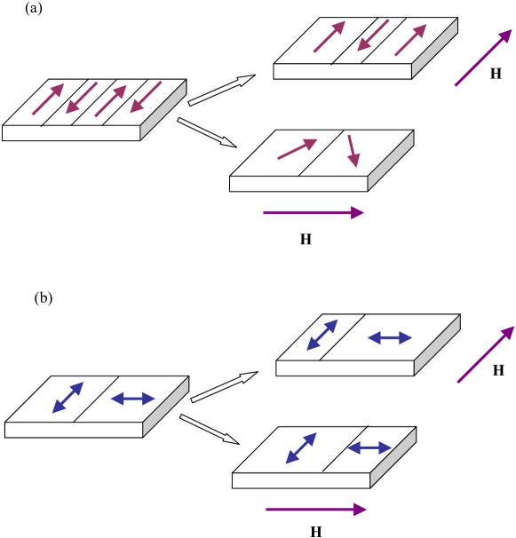
Figure 1: (Color online) Behavior of the FM (a) and AFM (b) domain structure in the external magnetic field $\mathbf{H}$. In the absence of field both types of domains (shown by arrows) are equally represented. (a) FM domains have opposite direction of magnetization vector. The magnetic field applied parallel to an easy axis (upper panel) removes degeneracy of the domains. As a result, fraction of the favorable domain increases. If $\mathbf{H}$ is perpendicular to the easy axis, domains of both types are equivalent, the domain fraction does not change, magnetic field induces a tilt of the magnetizations (lower panel). (b) AFM domains have different (perpendicular) orientations of AFM vectors. Degeneracy of the domains is removed for any of two mutually perpendicular orientations of the magnetic field.

The domain structure of FMs reconfigures in the magnetic field which is parallel to an easy axis and does not change if the magnetic field is perpendicular to this axis. Macroscopic magnetization of the sample (and hence, macroscopic susceptibility) is inversely proportional to the appropriate component of demagnetization tensor. In contrast, in antiferromagnetic crystals the DS reconfigures for both mutually perpendicular orientations of the magnetic field. Macroscopic magnetization depends upon the components of destressing tensor that have a magnetoelastic origin. So, a material that bears simultaneously the features of FM and AFM can show some new type of behavior in the external magnetic field governed by competition between the demagnetizing and destressing effects.

In the present paper we study an equilibrium DS of multiferroic Sr₂Cu₃O₄Cl₂ with the FM and AFM order parameters. In the framework of phenomenological approach we analyze the possible magnetization curves that could be obtained for the samples of different shape and different field treatment. On the basis of the developed model we make an attempt to interpret the unusual behavior of macroscopic magnetization observed in the experiments of Parks et al Parks:2001 and predict a peculiarity of the elastic properties of Sr₂Cu₃O₄Cl₂ at the temperature $T\approx 100$ K.

II Model

The crystal structure of high-temperature superconducting cuprates Sr₂Cu₃O₄Cl₂ and Ba₂Cu₃O₄Cl₂ consists of Cu₃O₄ planes separated by spacer layers of SrCl or BaCl Noro:1994 ; Kim:2001 ; Parks:2001 . Two types of magnetic ions, CuI and CuII (see Fig. 2) form two interpenetrating square lattices within Cu₃O₄ planes.

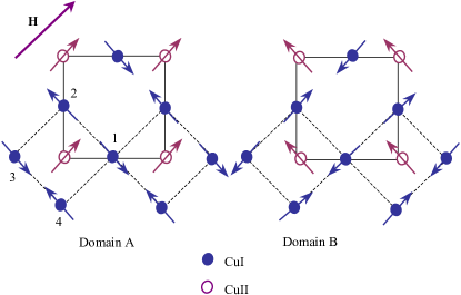
Figure 2: (Color online) Magnetic structure of Cu₃O₄ layer in two different configurations (domains). Magnetic field is parallel to $\langle 110\rangle$. Two types of magnetic ions are represented with the filled and hollow circles. FM ordered moments of CuII could be (a) parallel (domain A) or (b) perpendicular (domain B) to the applied magnetic field. Small canting of the CuI spins induced by the external magnetic field is not shown.

Within the temperature interval $T_{II}=40$ K$\leq T\leq T_{I}=380$ K the ions of the first type (CuI) are AFM ordered while the ions of the second type (CuII) bear small but nonzero FM moment. According to the experiments Kastner:1999, , mutual orientation of CuI and CuII moments depends upon the direction of the external magnetic field and can be either perpendicular or parallel. Thus, the magnetic structure consists of two weakly coupled subsystems, namely, an AFM, localized on CuI ions, and a FM one, localized on CuII ions. The FM subsystem is unambiguously described by the magnetization vector $\mathbf{M}_{\rm F}$ and the AFM subsystem is described by two vectors: AFM vector $\mathbf{L}=(\mathbf{S}_{1}-\mathbf{S}_{2}+\mathbf{S}_{3}-\mathbf{S}_{4})/4$ and ferromagnetic vector $\mathbf{M}=\sum_{j}\mathbf{S}_{j}/4$ (numeration of CuI sites is shown in Fig. 2).

In the absence of the external field the FM moments at CuII sites are oriented along $\langle 110\rangle$ crystal directions perpendicular to the staggered magnetizations of AFM subsystem, as shown in Fig. 2. Due to tetragonal symmetry of the crystal (space group $I4/mmm$) an equilibrium magnetic structure can be realized in four types of equivalent domains as shown in Figs. 2 and 3. Domains of type A and B could be thought of as AFM domains because they correspond to different orientations of $\mathbf{L}$ vector and thus are sensitive to orientation of the magnetic field $\mathbf{H}$ with respect to the crystal axes (see Fig. 1). Types A1 and A2 (and, correspondingly, B1 and B2) are FM domains, they have an opposite direction of $\mathbf{M}_{\rm F}$ vector and could be removed from the sample by $\mathbf{H}\|\mathbf{M}_{\rm F}$.

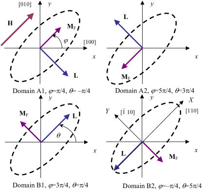
Figure 3: (Color online) Four types of magnetic domains. Axes $x$ and $y$ are parallel to $\langle 100\rangle$ crystal directions. The external magnetic field $\mathbf{H}\|[110]$ (if any). Types A and B have different orientations of AFM vector, types 1 and 2 correspond to opposite directions of FM vector $\mathbf{M}_{F}$. Ellipse (dash line) images the supposed shape of the sample and its orientation (axes $X$, $Y$) with respect to crystal axes.

Phenomenological description of the DS is based on the analysis of the free energy potential $\Phi$ of the sample. We take into account three constituents of $\Phi$: magnetic $\Phi_{\rm{mag}}$, stray (demagnetizing), $\Phi_{\rm{stray}}$ and destressing, $\Phi_{\rm{dest}}$, energy:

$$\Phi=\Phi_{\rm{mag}}+\Phi_{\rm{stray}}+\Phi_{\rm{dest}}.$$ (1)

Magnetic energy of Sr₂Cu₃O₄Cl₂ crystal in mean field approximation is well established Chou:1997 ; Kastner:1999 ; Kim:2001 and can be written as follows:

$$\Phi_{\rm{mag}} = \int_{V}dV\left\{\frac{4}{M_{0}^{2}}\left[J_{0}\left(\mathbf{M}^{2}-\mathbf{L}^{2}\right)+J_{\rm{av}}\mathbf{M}\cdot\mathbf{M}_{\rm F}+J_{\rm{pd}}\mathbf{M}_{\rm F}\hat{\sigma}_{z}\mathbf{L}+K_{\perp}L_{z}^{2}\right]\right.$$ (2)

$$- \left.\frac{8}{M_{0}^{4}}K_{\|}L_{x}^{2}L_{y}^{2}-\mathbf{H}\cdot\mathbf{M}_{\rm F}-2\mathbf{H}\cdot\mathbf{M}\right\}.$$

Here $V$ is the sample volume, $M_{0}$ is CuI sublattice magnetization, orthogonal axes $x$ and $y$ are parallel to the crystal directions [100] and [010], respectively (see Fig. 3). $\hat{\sigma}_{z}$ is the Pauli matrix. The meaning and values of phenomenological constants are given in Table 1. In the last column of this Table all the constants are converted to Oe by division by sublattice magnetization $M_{0}=27.4$ Gs (that corresponds to spin $s=1/2$ per CuI site).

Table 1: Parameters used in the free energy [Eq. (2)]. The second column gives the raw data (in meV) as taken from Refs.Chou:1997, ; Kastner:1999, ; Parks:2001, , in the last column the same values are given in Oe.

Parameter	Meaning	Value in meV	Value in Oe
$J_{0}$	CuI- CuI superexchange (in-plane)	130	1.02$\cdot 10^{7}$
$J_{\rm av}$	isotropic pseudodipolar interaction	-12	-9.4$\cdot 10^{5}$
$J_{\rm pd}$	anisotropic pseudodipolar interaction	-0.027	-2.1$\cdot 10^{3}$
$K_{\perp}$	out-of-plane anisotropyKim:2001	0.068	$5.3\cdot 10^{3}$
$K_{\|}$	in-plane anisotropy	10$\cdot 10^{-6}$	7.8$\cdot 10^{-2}$

Contributions $\Phi_{\rm{stray}}$ and $\Phi_{\rm{dest}}$ in Exp. (1) arise from the long-range dipole-dipole interactions of the magnetic and magnetoelastic nature, correspondingly, and depend upon the sample shape. We consider a thin (thickness $c$) pillar with an elliptic crossection whose principal axes $X$ and $Y$ are parallel to $\langle 110\rangle$ directions within the Cu₃O₄ layers (see Fig. 3). In this case

$$\Phi_{\rm{stray}}=\frac{V}{2}\left[N^{\rm{dm}}_{a}\langle M_{\rm{F}X}+2M_{X}\rangle^{2}+N^{\rm{dm}}_{b}\langle M_{\rm{F}Y}+2M_{Y}\rangle^{2}\right],$$ (3)

where the brackets $\langle\ldots\rangle$ mean averaging over the sample volume. The components of demagnetization tensor $N^{\rm{dm}}_{a,b}$ are calculated in a standard way Bar:1968E :

$$N^{\rm{dm}}_{a}=\frac{4\pi c}{a\sqrt{1-k^{2}}}\int_{0}^{\pi/2}\frac{\sin^{2}\phi d\phi}{\sqrt{1-k^{2}\sin^{2}\phi}};\quad N^{\rm{dm}}_{b}=\frac{4\pi c\sqrt{1-k^{2}}}{a}\int_{0}^{\pi/2}\frac{\cos^{2}\phi d\phi}{\sqrt{1-k^{2}\sin^{2}\phi}}.$$ (4)

Here $a\geq b(\gg c)$ are the ellipse’s semiaxes (parallel to $X$ and $Y$ axes) and the parameter $k^{2}=1-b^{2}/a^{2}$ depends upon an aspect ratio $b/a$ of the sample.

The destressing energy can be written in an analogous form gomonay:174439

$$\Phi^{\rm dest} = V\left\{N^{\rm des}_{\rm is}[\langle L_{Y}^{2}-L_{X}^{2}\rangle^{2}+4\langle L_{X}L_{Y}\rangle^{2}]\right.$$ (5)

$$+ \left.N^{\rm des}_{\rm 2an}\langle L_{X}^{2}-L_{Y}^{2}\rangle-N^{\rm des}_{\rm 4an}[\langle L_{X}^{2}-L_{Y}^{2}\rangle^{2}-4\langle L_{X}L_{Y}\rangle^{2}]\right\}.$$

An explicit form of the destressing constants $N^{\rm des}$ depends upon the elastic and magnetoelastic properties of the crystal which we assume to be isotropic (that means, in particular, the following relation between the elastic modula: $c_{11}-c_{12}=2c_{44}$). Then,

$$N^{\rm des}_{\rm is}=\frac{\lambda^{2}(3-4\nu)}{16c_{44}(1-\nu)},\quad N^{\rm des}_{2}=\frac{c}{b}\cdot\frac{[\lambda^{2}(2-3\nu)+\lambda_{v}\lambda]J_{2}(k)}{8c_{44}(1-\nu)},\quad N^{\rm des}_{\rm 4an}=\frac{c}{b}\cdot\frac{\lambda^{2}J_{4}(k)}{3c_{44}(1-\nu)},$$ (6)

where $\lambda$ and $\lambda_{v}$ are magnetoelastic constants,$\nu=c_{12}/(c_{11}+c_{12})$ is the Poisson ratio and we have introduced the dimensionless shape-factors $J_{2,4}(k)$ as follows gomonay:174439

$$J_{2}(k) = \int_{0}^{\pi/2}\frac{(\sin^{2}\phi+\cos 2\phi/k^{2})d\phi}{\sqrt{1-k^{2}\sin^{2}\phi}},$$

$$J_{4}(k) = \int_{0}^{\pi/2}\frac{(1-8\cos 2\phi-k^{2}\sin^{2}\phi+8\cos 2\phi/k^{2})d\phi}{\sqrt{1-k^{2}\sin^{2}\phi}}.$$ (7)

In Eqs.(3) and (5) we have omitted $Z$($\|z\|[001]$)-components of the demagnetizing and destressing tensors as inessential for further consideration.

Expressions (2), (3), and (5) could be substantially simplified if one takes into account that: i) far below the Néel temperature the values of sublattice magnetizations $M_{0}$ and $M_{\rm F}$ are saturated and constant; as a result ii) $\mathbf{L}\perp\mathbf{M}$ and $\mathbf{L}^{2}+\mathbf{M}^{2}=M_{0}^{2}$ (normalization conditions); iii) if the magnetic field is much smaller than the spin-flip field, $H\ll J_{0}/M_{0}$ and coupling between the FM and AFM subsystems is much smaller than AFM exchange, $J_{\rm av}M_{F}\ll J_{0}M_{0}$, the magnetization induced in AFM subsystem is small, $M\ll M_{0}$, and vector $\mathbf{M}$ can be excluded from Eq. (2) as follows Kosevich:1983 :

$$\mathbf{M}=\frac{1}{8J_{0}}\left[\mathbf{L}\times\left[\left(\mathbf{H}-2\frac{J_{\rm av}}{M_{0}^{2}}\mathbf{M}_{\rm F}\right)\right]\right];$$ (8)

iv) if out-of-plane anisotropy is strong enough, $K_{\perp}\gg K_{\|}$ (see Table 1), all the magnetic vectors lie within $xy$ (and, equivalently, $XY$) plane and could be described with the only angle variable, as shown in Fig. 3:

$$L_{x}=M_{0}\cos\theta,\,L_{y}=M_{0}\sin\theta;\,M_{{\rm F}x}=m_{\rm F}M_{0}\cos\varphi,\,M_{{\rm F}y}=m_{\rm F}M_{0}\sin\varphi.$$ (9)

Here $m_{\rm F}$(=$10^{-3}$ for Sr₂Cu₃O₄Cl₂ Kastner:1999 ) is a dimensionless constant that represents the ratio between the spin moments localized on CuII and CuI sites.

With account of the relations (8) and (9) the specific potential $\phi\equiv\Phi/V$ (see Exp. (1) takes the following form

$$\phi = 4J_{\rm{pd}}m_{\rm F}\langle\cos(\theta+\varphi)\rangle+K_{\|}\langle\cos 4\theta\rangle-\frac{J^{2}_{\rm{av}}}{8J_{0}}m^{2}_{\rm F}\langle\cos 2(\theta-\varphi)\rangle$$

$$- m_{\rm F}H\left[\left(1-\frac{J_{\rm{av}}}{8J_{0}}\right)\langle\cos(\varphi-\psi)\rangle+\frac{J_{\rm{av}}}{8J_{0}}\langle\cos(2\theta-\psi-\varphi)\rangle\right]+\frac{H^{2}}{32J_{0}}\langle\cos 2(\theta-\psi)\rangle$$

$$- N^{\rm des}_{\rm 2an}\langle\cos 2(\theta-\psi)\rangle+\frac{1}{2}M_{0}m_{\rm F}^{2}\left[N^{\rm{dm}}_{a}\langle\cos(\varphi-\psi)\rangle^{2}+N^{\rm{dm}}_{b}\langle\sin(\varphi-\psi)\rangle^{2}\right]$$

$$+ N^{\rm des}\langle\cos 2(\theta-\psi)\rangle^{2}+\Delta N^{\rm des}\langle\sin 2(\theta-\psi)\rangle^{2}.$$

where $\psi$ is an angle between the magnetic field and $x$-axis, $N^{\rm des}\equiv N^{\rm des}_{\rm is}+N^{\rm des}_{\rm 4an}$, $\Delta N^{\rm des}\equiv 4\left(N^{\rm des}_{\rm is}-N^{\rm des}_{\rm 4an}\right)$, and we assume that the field is parallel to one of the principal axes of the sample (this corresponds to the experimental situation that will be discussed below). Here and for the rest of the paper we use the values in Oe (see the last column of Table 1) instead of energy units (say, $\phi\rightarrow\phi/M_{0}$, etc.).

Let us consider the case when the magnetic field is parallel to one of the easy axes, $\mathbf{H}\|[110]$, so, $\psi=\pi/4$. In an infinite sample (all the components of tensors $N^{\rm{dm}},N^{\rm des}$ are equal to zero) minimization of $\phi$ with respect to magnetic variables $\theta$ and $\varphi$ gives rise to the four solutions labeled as A1,2 and B1,2 (see Fig. 3). Equilibrium values at $H=0$ are

$${\textrm{state A1}}:\qquad\theta_{\rm A1}=-\pi/4,\qquad\varphi_{\rm A1}=\phantom{3}\pi/4;$$

$${\textrm{state B1}}:\qquad\theta_{\rm B1}=\phantom{3}\pi/4,\qquad\varphi_{\rm B1}=3\pi/4;$$ (11)

$${\textrm{state A2}}:\qquad\theta_{\rm A2}=3\pi/4,\qquad\varphi_{\rm A2}=5\pi/4;$$

$${\textrm{state B2}}:\qquad\theta_{\rm B2}=5\pi/4,\qquad\varphi_{\rm B2}=-\pi/4.$$

It should be stressed that in contrast to pure AFMs the configurations with $(\mathbf{M}_{F},\mathbf{L})$ and $(\mathbf{M}_{F},-\mathbf{L})$ are inequivalent, due to anisotropic pseudodipolar interactions (described by the constant $J_{\rm pd}$).

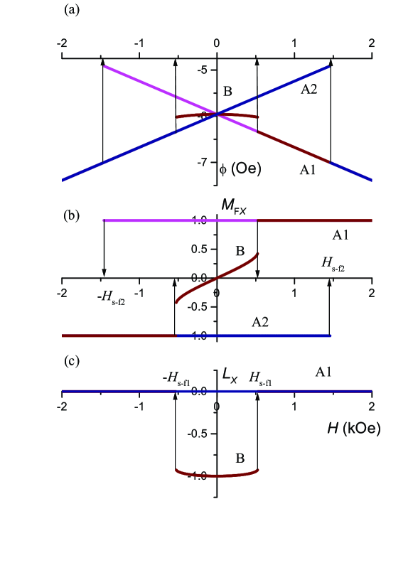
Figure 4: (Color online) Stability ranges of homogeneous configurations shown in Fig. 3 in the external magnetic field $\mathbf{H}\|[110]$. (a) Specific energy (in Oe) of equilibrium homogeneous state vs $H$. (b), (c) Normalized projections of FM and AFM moments on the field direction. Field induces rather noticeable rotation of $\mathbf{M}_{\rm F}$ vector toward the field direction (b) and slight tilt of $\mathbf{L}$ vector (c). Loss of stability takes place at the critical values $H=H_{\rm s-f1,2}$, as shown with arrows.

Fig. 4 illustrates the field-induced variation of equilibrium magnetic configurations (represented by $X$-projections of $\mathbf{M}_{\rm F}$ and $\mathbf{L}$ vectors) obtained from the numerical minimization of the Exp. (II) using the data from Table 1. It is clearly seen that within the interval $|H|\leq H_{\rm s-f1}=525$ Oe there exist all four states A1,2 and B1,2. The magnetic field removes degeneracy between the states A1, A2 and B, as can be seen from Fig. 4a. In particular, when $H\geq 0$, the specific energies $\phi_{j}\equiv\phi(\theta_{j},\varphi_{j})$ of equilibrium states are related as follows: $\phi_{\rm A1}<\phi_{\rm B}<\phi_{\rm A2}$. So, in some cases (discussed below) variation of the external field may induce formation of the AFM (B) instead of the FM (A2) domain. Orientations of $\mathbf{M}_{\rm F}$ and $\mathbf{L}$ vectors in the A states are not influenced by the field, while in the B states both vectors are slightly tilted (see Fig. 4b,c). Rotation of AFM vector from the field direction in the state B (where $\mathbf{H}\|\mathbf{L}$) is a peculiar feature of the FM+AFM multiferroic caused by pseudodipolar interactions between CuI and CuII ions. In the pure antiferromagnets an AFM vector $\mathbf{L}$ keeps parallel (with respect to $\mathbf{H}$) orientation up to the field of spin-flop transition.

The first critical field $H_{\rm s-f1}\propto\sqrt{J_{0}K_{\|}}$ corresponds to a step-like (spin-flop) transition B1,2$\rightarrow$A1. In the interval $H_{\rm s-f1}<|H|<H_{\rm s-f2}=1465$ Oe the potential $\Phi$ has only two minima that correspond to the states A1 and A2. The second critical field $H_{\rm s-f2}$ corresponds to 180^∘ switching of $\mathbf{M}_{\rm F}$ vector. Its value depends on the effective anisotropy that originates from the pseudodipolar coupling (corresponding constants $J_{\rm av},J_{\rm pd}$) and in-plane anisotropy $K_{\|}$ and can be calculated only numerically. Above $H\geq H_{\rm s-f2}$ the sample is in a single domain state (A1).

III Equilibrium domain structure and magnetization curves

On the large scales (much greater than the characteristic scale of the magnetic inhomogeneity, i.e., domain wall thickness) the magnetic structure of the sample is represented by a set of magnetic variables $\{\theta_{j},\varphi_{j}\}$ that describes orientation of FM and AFM vectors inside the domains ($j=$A1, A2, B1, B2) and a set of variables $\{\xi_{j}\}$ that represents the amount of matter (say, volume fraction) in the state of $j$-type (obviously, $\sum\xi_{j}=1$). Equilibrium DS in presence of the external field is then found from the condition of minimum of $\Phi$ with respect to $\{\theta_{j},\varphi_{j},\xi_{j}\}$.

In such an approach one can neglect a contribution of the domain walls into free energy potential $\Phi$. However, we implicitly account for the inhomogeneities in space distribution of the FM and AFM vectors when we chose independent variables for the potential $\Phi$. Namely, reconstruction of the DS may proceed in two ways: i) by the field-induced motion of the domain walls; ii) by nucleation and growth of the energetically favorable domains. The first way is almost activation-less while in the second case the system should overcome the potential barrier related with the formation of the domain walls. In the case under consideration the domain walls between AFM (A/B) and FM (A1/A2 or B1/B2) domains have different energies, and so, appear at different conditions. In what follows we consider some typical situations and show the way to control the DS with appropriate treatment of the sample.

III.1 Four types of domains

In the case when all four types of domains may freely grow or diminish in size (say, in a virgin sample that initially contains domains of all types), the external magnetic field is screened by an appropriate domain configuration (see Fig. 5) and the effective field inside the sample is zero. Equilibrium values of the magnetic variables in this case are given by Eq. (II) and the domain fractions depend on magnetic field as follows:

$$\xi_{\rm A1,A2}=\frac{1}{4}\left[1-\xi^{(0)}\pm\frac{2H}{H_{\rm dm}}+\left(\frac{H}{H_{\rm des}}\right)^{2}\right];\quad\xi_{\rm B1}=\xi_{\rm B2}=\frac{1}{4}\left[1+\xi^{(0)}-\left(\frac{H}{H_{\rm des}}\right)^{2}\right],$$ (12)

where we have introduced the demagnetizing, $H_{\rm dm}$, and the destressing, $H_{\rm des}$, fields:

$$H_{\rm dm}\equiv m_{\rm F}N^{\rm{dm}}_{a}M_{0},\quad H_{\rm des}\equiv 8\sqrt{J_{0}N^{\rm des}}.$$ (13)

As seen from Eq. (13), the value of destressing field is enhanced due to exchange interactions (constant $J_{0}$). On the contrary, the demagnetizing field is weakened due to small FM moment ($m_{\rm F}\ll 1$). So, in the crystal under consideration the demagnetizing effects are much smaller than the destressing ones, $H_{\rm dm}\ll H_{\rm des}$ (see Table 2).

The value $\xi^{(0)}$ introduced in Eq. (12) represents the disbalance between type A and type B domains in the absence of field. This value depends upon the shape of the sample (or, equivalently, from the aspect ratio, see Eq. (6)):

$$\xi^{(0)}\equiv\frac{N^{\rm des}_{\rm 2an}}{N^{\rm des}}\approx\frac{c}{b}J_{2}(k).$$ (14)

Such a shape-induced nonequivalence of domains has a magnetoelastic origin (see Ref.gomonay:174439, for details) and originates from the AFM properties of the system. The disbalance between type A and type B domains was noticed in the experiments Ref.Parks:2001, for the different sample shapes. The value $\xi^{(0)}=0.22$ calculated from Eq.(14) for the typical sample size (see Table 2) fits well the experimental magnetization curves, as we will see below.

The described configuration of the DS (see Eq. (12)) is schematically shown in Fig. 5b. The fraction of the unfavourable domains A2, B1 and B2 diminishes and at the critical value

$$H=H_{\rm cr1}\equiv\frac{H^{2}_{\rm des}}{H_{\rm dm}}\left[1-\sqrt{1-(1-\xi^{(0)})\left(\frac{H_{\rm dm}}{H_{\rm des}}\right)^{2}}\right]\approx\frac{1}{2}(1-\xi^{(0)})H_{\rm dm}$$ (15)

the unfavourable FM domains A2 disappears ($\xi_{\rm A2}=0$).

At $H\geq H_{\rm cr1}$ the internal effective magnetic field is nonzero and magnetizations in the domains of B type rotate. However, if $H_{\rm cr1}\ll H_{\rm s-f}$ (as, indeed the case in the crystal under consideration), small tilt of $\mathbf{M}_{\rm F}$ and $\mathbf{L}$ vectors can be neglected and field dependence of the domain fractions (shown in Fig. 5c) is approximated as

$$\xi_{\rm A1}=\frac{1}{2}\left[1-\xi^{(0)}+\frac{16Hm_{\rm F}J_{0}}{H^{2}_{\rm des}}+\left(\frac{H}{H_{\rm des}}\right)^{2}\right],\quad\xi_{\rm B1,2}=\frac{1}{4}\left[1+\xi^{(0)}-\frac{16Hm_{\rm F}J_{0}}{H^{2}_{\rm des}}-\left(\frac{H}{H_{\rm des}}\right)^{2}\right].$$ (16)

The second critical field at which the unfavourable domains of B type disappear ($\xi_{\rm B1,2}=0$) is given by the expression

$$H_{\rm cr2}\equiv 8m_{\rm F}J_{0}\left[\sqrt{1+\left(\frac{H_{\rm des}}{8m_{\rm F}J_{0}}\right)^{2}\left(1+\xi^{(0)}\right)}-1\right]\approx\frac{2N^{\rm des}}{m_{\rm F}}\left(1+\xi^{(0)}\right).$$ (17)

Above the second critical field, $H\geq H_{\rm cr2}$, the sample is a single domain (A1) in average, with the possible remnants of the states A2, B and corresponding domain walls that can serve as the nucleation centers during the field cycling. Full monodomainization of the sample takes place above the critical field $H_{\rm s-f2}\gg H_{\rm cr2}$ at which all the states except A1 became unstable.

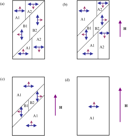
Figure 5: (Color online) Behavior of the combined FM and AFM domain structure in the external magnetic field $\mathbf{H}\|$[110] (parallel to the long side of the sample). (a) In the field absence all types of domains (A1, A2, B1, B2) are equally represented, the disbalance $\xi^{(0)}$ between A and B types depends upon the aspect ratio of the sample. (b) Below the first critical field, $H\leq H_{\rm cr1}$, the domains are rearranged in such a way that the effective magnetic field vanishes. (c) In the interval $H_{\rm cr1}\leq H\leq H_{\rm cr2}$ the unfavourable domains of A2 type disappear, A1-domains compete with the domains of B-type. (d) Above the second critical field, $H>H_{\rm cr2}$, the sample is a single domain.

Field cycling of the sample that initially had all the types of domains is reversible if the maximal field value $H_{\rm max}$ is not very large, $H_{\rm cr2}\leq H_{\rm max}\ll H_{\rm s-f2}$. Macroscopic magnetization is parallel to the direction of the external field due to the full compensation of the perpendicular component by B1 and B2 domains.

Table 2: Parameters used in numerical simulations. The source of data (experimental or calculated) is specified in the last column.

Parameter	Meaning	Value	Rem
$a\times b\times c$	Sample size	$7\times 2\times 0.5$ mm3	Ref.Parks:2001,
$m_{F}$	$M_{F}/M_{0}$	$7\cdot 10^{-4}$	Ref.Kim:2001,
$M_{F}$	Saturation magnetization	$7\cdot 10^{-3}$ emu/g	Ref.Parks:2001,
$\xi^{(0)}$	Shape-induced bias	0.22	Eq.(14)
$H_{\rm dm}$	Demagnetization field	0.3 Oe	Eq.(13)
$N^{\rm des}$	Destressing const., $T=120$K	$7$ mOe	Fitting
	$T=100$ K	1.5 mOe	param.
$H_{\rm des}$	Destressing field, $T=120$ K	$2.1$ kOe	Eq.(13)
	$T=100$ K	$1.1$ kOe

Field dependence of macroscopic magnetization $M_{\rm par}\propto(\xi_{\rm A1}-\xi_{\rm A2})$ at $T=120$ K calculated from Eqs. (12) and (16) (see Tables 1 and 2) is represented in Fig. 6. One can distinguish three intervals that correspond to different domain composition: i) steep growth of $M_{\rm par}$ from 0 to $\propto 0.5(1-\xi^{(0)})M_{\rm F}$ (at $H=H_{\rm cr1}$) due to the motion of A1/A2 domain walls initiated by demagnetization; ii) smooth growth of $M_{\rm par}$ from $\propto 0.5(1-\xi^{(0)})M_{\rm F}$ to $\approx M_{\rm F}$ (at $H=H_{\rm cr2}$) due to the motion of A1/B domain walls initiated by the destressing; iii) very smooth growth of $M_{\rm par}$ due to rotation of sublattice magnetizations (not seen in Fig. 6). Such a behavior contrasts with a “standard” magnetization curve of FM and also with the case when only two types of domains could compete under the action of external field. The last case will be considered in details in the next section.

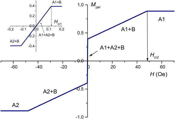
Figure 6: (Color online) Magnetization curve (projection on field direction) in the external magnetic field $\mathbf{H}\|$[110] for the case depicted in Fig. 5. Inset shows the details of magnetization behavior below $H_{\rm cr1}$. The jogs (shown with arrows) arise at the critical fields $H=H_{\rm cr1,2}$ when one type of domains disappear. Magnetization is normalized to saturation value.

III.2 Competition of two domains

Let us consider a sample that was preliminary monodomainized to the state A1 by excursion into the region of high field, $H\geq H_{\rm s-f2}$. The DS in this case depends upon the relation between nucleation energies of different states. As it was shown above, at $H>0$ an AFM domain B is more favorable than a FM domain A2 (see Fig. 4a). If, in addition, there is a slight misalignment between the magnetic field $\mathbf{H}$ and a crystal axis [110] that removes degeneracy between the B1 and B2 states, the DS of the sample is represented by the domains of only two types, A1 and B1.

Equilibrium values of the magnetic variables in this case were calculated by the numerical minimization of the potential (II) with limitations $\xi_{A2}=\xi_{B2}=0$. The values of the destressing coefficient $N^{\rm des}$ at different temperatures (see Table 2) were defined from the fitting of experimental data Parks:2001 .

Field dependence of macroscopic the magnetization at $T=120$ K is shown in Fig. 7 with solid lines. Points represent experimental data Parks:2001 . Due to the fact that the domains A1 and B1 could not screen the external field, the macroscopic magnetization has two components: one that is parallel to $\mathbf{H}$ (upper panel in Fig. 7) and one that is perpendicular to $\mathbf{H}$ (lower panel). The parallel and perpendicular components represent the fractions of A1 and B1 domains, respectively.

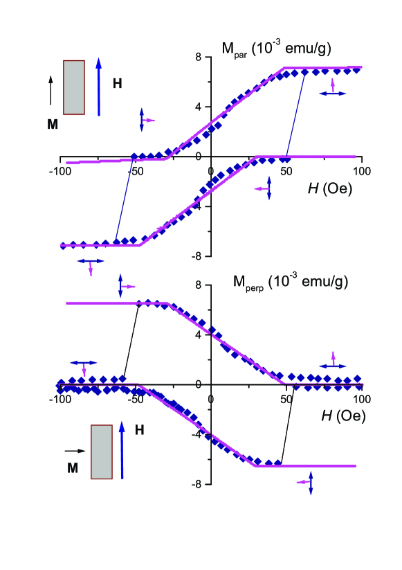
Figure 7: (Color online) Macroscopic magnetization vs magnetic field. Points – experimental data for Sr₂Cu₃O₄Cl₂ Parks:2001 taken at $T=$120 K after monodomainization of the sample at high fields $H\propto 5$ T. Solid lines – theoretical approximation (see text for details). Upper and lower panels show, correspondingly, the parallel and perpendicular components of magnetization with respect to magnetic field. Insets show geometry of the experiment: orientation of the field with respect to the sample and orientation of the measured magnetization with respect to $\mathbf{H}$. The dominant type of domains for each field interval is depicted schematically by the single- and double-headed arrows.

When the field decreases from high positive values, an AFM domains of B type appear and magnetizations $M_{\rm par}(H)$ and $M_{\rm perp}(H)$ vary smoothly between zero and saturation value. The slope of magnetization curves depends upon the destressing coefficient and is thus much smaller than the initial steep slope in the 4-domain case (see Fig. 6). At small negative field the sample is almost a single domain (type B). However, this state is a metastable one from the energy point of view, as seen from Figs.8 and 4a. Really, below $H=H_{3}\approx 2.8$ Oe (marked with arrow in Fig.8) the energy of the state A2 (with $\mathbf{M}_{F}\uparrow\downarrow\mathbf{H}$) is lower than that of a single domain state B1 and a multidomain state A1+B1. On the other hand, due to preliminary high-field treatment, the sample contains no nucleation centers of A2 state. So, the states B1 and A2 are separated with the potential barrier that could be overcome only at $H=H_{2}\approx-50$ Oe (according to Ref.Parks:2001, , this value varies from sample to sample and depends on temperature). After the subsequent excursion into high negative fields (well below $H_{2}$) the sample transforms into a single domain A2 and one can observe competition between the A2 and B2 domains during the further field increase.

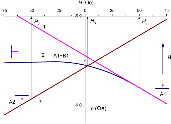
Figure 8: (Color online) Magnetic energy vs magnetic field, $T=120$ K. Lines 1 and 3 correspond to a single domain state (domains A1 and A2, correspondingly), line 2 represents equilibrium two-domain state (domains A1 and B1). Domain B1 appears at $H=H_{1}$. Domain A2 appears at field $H=H_{2}$ (determined empirically) when the energy difference between two-domain and single domain states is enough for nucleation of this energetically favorable domain. At $H=H_{3}$ the energy of two-domain state is equal to the energy of a single-domain state A2, but the potential barrier between two states prevents nucleation of the domain A2.

III.3 Domain structure and field treatment

In the previous subsections we have considered two limiting cases of field treatment that result in two types of magnetization curves. In the virgin sample (no field treatment) the magnetization can be smoothly and reversibly changed between two opposite directions. Field cycling between high fields (high enough to remove all the domain walls and the remains of unfavorable domains) results in a hysteretic behavior when magnetization varies smoothly between zero and saturation value and then suddenly changes due to transition from metastable to stable state.

In this subsection we consider some intermediate case when a single domain sample is cycled in low fields. Corresponding magnetization curve is shown in Fig. 9a (solid lines – numerical simulations, points – experimental data Parks:2001 , $T=100$ K). Field cycling starts at high positive fields, where the sample is a single domain. When the field is decreased down to $H=H_{1}$ (see Fig. 8a) the domains of B1 type appear and the DS consists of A1 and B1 domains. Magnetization curve (upper curve in Fig. 9a) in this case is of two-domain type discussed in Subsection III.2 (we still assume slight misalignment that excludes one type of B domains). However, further behavior of the DS and hence, magnetization, depends upon the size of the loop. If the loop is small ($|H|\leq|H_{2}|$, where $H_{2}$ is a coercive field at which domain B1 transforms into A2 as explained above), magnetization varies smoothly between zero value at negative fields and saturation value at positive fields. If the loop is very large ($|H|\geq|H_{\rm cr2}|$), the DS structure consists of two domains: A1 and B1 for large positive and small negative fields and A2 and B2 for large negative and small positive fields, as shown in Figs. 9b and 7. In the intermediate case ($|H_{2}|\leq|H|\ll|H_{\rm cr2}|$) the DS includes three types of domains, A1, A2 and B2 (lower curve in Fig. 9a), and magnetization curve is asymmetric. It is worth to note that theoretical magnetization curves calculated with only one fitting parameter (destressing coefficient $N^{\rm des}$) fit well experimental data, as seen from Figs.9 and 7.

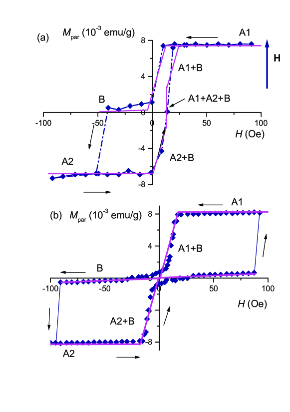
Figure 9: (Color online) Macroscopic magnetization vs magnetic field for different field treatment. Points – experimental data for Sr₂Cu₃O₄Cl₂ Parks:2001 taken at $T=$100 K (see text for details), solid lines – theoretical approximations. Thin arrows show the direction of field sweeping. (a) Competition between FM and AFM domain structure. Field treatment starts from the high positive values ($H\approx 1$ T) where the sample is a single domain. Variation of field is swept at intermediate value $|H_{2}|\leq|H|\ll|H_{\rm cr2}|$, large enough to induce switching between metastable, B1, and stable, A2, states and small enough to remove the traces of A1 and B1 phases from the sample. (b) Hysteresis loop with the excursion into high fields. For any field value the DS includes only two types of domains, as in Fig. 7. Only parallel component of magnetization is shown.

IV Discussion

We have considered the different types of the DS behavior in a multiferroic with AFM and FM order parameters. Depending on the field treatment the DS may include from one to four types of domains and can be unambiguously determined from the magnetization curves in the field $\mathbf{H}\|[110]$. Namely, if DS includes all types of domains, macroscopic magnetization is parallel to $\mathbf{H}$, magnetization curve is reversible, varies between $\pm$ saturation value, and includes steep section at small fields. If the DS includes three types of domains A1, A2 and B1, the macroscopic magnetization has two components, parallel, $M_{\rm par}$, and perpendicular, $M_{\rm perp}$, to $\mathbf{H}$. During field cycling $M_{\rm par}$ varies between positive and negative saturation values, while $M_{\rm perp}$ varies between zero and saturation value. At last, if the DS includes only two domains, A and B, both $M_{\rm par}$ and $M_{\rm perp}$ vary between zero and saturation value.

We argue that formation of AFM (B) domain results from the destressing effect which, in turn, originates from magnetoelastic interactions. An absolute value of magnetoelastic constant is rather small (compared to such AFMs as NiO, KCoF₃, etc) and corresponds to spontaneous strain $u\propto 10^{-6}$ (for estimation we took $c_{44}=20$ GPa at $T=120$ K). Such a small value of $u$ explains the low potential barrier for formation of AFM domains.

Analysis of magnetization curves shows that low-field susceptibility $\chi$ of the sample that consists of AFM domains is inversely proportional to the destressing coefficient $N^{\rm des}$ (in contrast to FM, where $\chi$ depends upon demagnetization constant). According to the experiments Parks:2001 , the inverse susceptibility $\chi^{-1}$ of Sr₂Cu₃O₄Cl₂ shows nontrivial temperature dependence (see Fig.10b) and attains the minimum at $T=T_{0}=97$ K. The domain fraction $\xi_{\rm A1}$ at fixed $\mathbf{H}$ extracted from the neutron scattering experiments of the reminded group Parks:2001 shows the same temperature dependence as $\chi$, as can be seen from Fig.10b. Using correlation between $N^{\rm des}$ and $\chi$ we predict the following temperature dependence of the destressing coefficient depicted in Fig.10a:

$$N^{\rm des}(T)=\left\{\begin{array}[]{cc}7.3\cdot 10^{-5}\cdot(T-T_{0}),&T\geq T_{0},\\ 6.13\cdot 10^{-5}\cdot(T_{0}-T),&T<T_{0}.\end{array}\right.$$ (18)

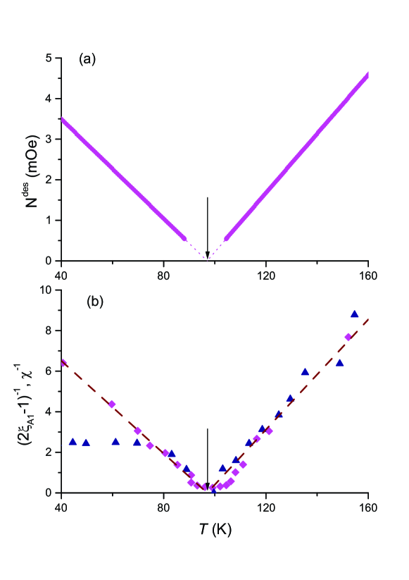
Figure 10: (Color online) Temperature dependence (a) of the destressing coefficient $N^{\rm des}$ predicted from the comparison with the (b) temperature dependence of the reciprocal domain A1 fraction $(2\xi_{\rm A1}-1)^{-1}$ (triangles) and the inverse susceptibility $\chi^{-1}$ (diamonds) plotted according to data Parks:2001 . Raw data for $\chi^{-1}$ were normalized (multiplied by appropriate factor) to fall into the same ranges of values as $(2\xi_{\rm A1}-1)^{-1}$. Dash line shows linear approximation of the experimental data. Peculiarity at $T=97$ K is indicated with arrow.

If we take into account that $N^{\rm des}\propto\lambda^{2}/c_{44}$ (see Eq.(6)) we may also anticipate a peculiarity of the elastic (or magnetoelastic) properties of the crystal in the vicinity of $T=T_{0}$.

In summary, we described the possible scenario of field-induced restructurization of the domains in the system that consists of the domains of different physical nature. The proposed model can be extended to multiferroics that show simultaneously ferroelectric and AFM ordering and also to FM martensites with ferroelastc and ferrpmagnetic ordering.

- (1) M. Gajek, M. Bibes, S. Fusil, K. Bouzehouane, J. Fontcuberta, A. Barthelemy, and A. Fert, Nature Mat. 6, 296 (Apr 2007)
- (2) C. R. dela Cruz, B. Lorenz, Y. Y. Sun, C. W. Chu, S. Park, and S.-W. Cheong, Phys. Rev. B 74, 180402(R) (2006)
- (3) V. A. Chernenko, A. Amengual, E. Cesari, V. V. Kokorin, and I. K. Zasimchuk, J. Phys. IV, Colloq 5, 95 (1995)
- (4) R. Ramesh and N. A. Spaldin, Nature Mat 6, 21 (2007)
- (5) Y.-H. Chu, L. W. Martin, M. B. Holcomb, and R. Ramesh, Materials Today 10, 16 (2007)
- (6) R. de Sousa and J. E. Moore, J.Nanoelectron.Optoelectron. 3, 77 (2008).
- (7) M. Fiebig, T. Lottermoser, D. Fröhlich, A. V. Goltsev, and R. V. Pisarev, Nature 419, 818 820 (2002)
- (8) C. Kittel, Rev. Mod. Phys. 21, 541 (Oct 1949)
- (9) In general, FM materials also show magnetoelastic coupling. However, anisotropic magnetostriction in AFM may have an exchange origin and thus may be much larger than that in FM. Moreover, in contrast to AFM, ferromagnetic domains with opposite direction of magnetization could be easily distinguished by the magnetic field but show the same magnetoelastic strain.
- (10) H. V. Gomonay and V. M. Loktev, Phys. Rev. B 75, 174439 (2007).
- (11) V. A. L’vov, E. V. Gomonaj, and V. A. Chernenko, Jour. of Phys.: Cond. Matt. 10, 4587 (1998)
- (12) Ferromagnets with the pronounced magnetostriction may also show nontrivial DS. In contrast to FM martensites, the DS in such materials consists of the domains that can be appropriately described by one (and only one) order parameter, magnetization or strain tensor component.
- (13) K. Ullakko, J. K. Huang, C. Kantner, R. C. O’Handley, and V. V. Kokorin, Appl. Phys. Lett 69, 1966 (1996).
- (14) B. Parks, M. A. Kastner, Y. J. Kim, A. B. Harris, F. C. Chou, O. Entin-Wohlman, and A. Aharony, Phys. Rev. B 63, 134433 (2001)
- (15) S. Noro, T. Kouchi, H. Harada, T. Yamadaya, M. Tadokoro, and H. Suzuki, Materials Science and Engineering: B 25, 167 (1994)
- (16) Y. J. Kim, R. J. Birgeneau, F. C. Chou, M. Greven, M. A. Kastner, Y. S. Lee, B. O. Wells, A. Aharony, O. Entin-Wohlman, I. Y. Korenblit, A. B. Harris, R. W. Erwin, and G. Shirane, Phys. Rev. B 64, 024435 (2001)
- (17) According to Ref.\rev@citealpnumKastner:1999, the FM moments at CuII ions result from the anisotropic “pseudodipolar” interactions between CuI and CuII.
- (18) M. A. Kastner, A. Aharony, R. J. Birgeneau, F. C. Chou, O. Entin-Wohlman, M. Greven, A. B. Harris, Y. J. Kim, Y. S. Lee, M. E. Parks, and Q. Zhu, Phys. Rev. B 59, 14702 (1999)
- (19) F. C. Chou, A. Aharony, R. J. Birgeneau, O. Entin-Wohlman, M. Greven, A. B. Harris, M. A. Kastner, Y. J. Kim, D. S. Kleinberg, Y. S. Lee, and Q. Zhu, Phys. Rev. Lett. 78, 535 (1997)
- (20) A. I. Akhiezer, V. G. Bar’yakhtar, and S. V. Peletminskii, Spin Waves, Interscience (Wiley) ed., North-Holland Series in Low Temperature Physics, Vol. 1 (North-Holland, Amsterdam, 1968)
- (21) A. M. Kosevich, B. A. Ivanov, and A. S. Kovalev, Nonlinear magnetization waves. Dynamical and topological solitons (Naukova dumka, Kiev, 1983) 192 p.
- (22) States B1 and B2 are equivalent in the field parallel to [110] direction.