Clustering properties of galaxies selected in stellar mass: Breaking down the link between luminous and dark matter in massive galaxies from $\mathbf{z=0}$ to $\mathbf{z=2}$

Abstract

We present a study on the clustering of a stellar mass selected sample of 18,482 galaxies with stellar masses $M_{*}>10^{10}$$M_{\odot}\,$at redshifts $0.4<z<2.0$, taken from the Palomar Observatory Wide-field Infrared Survey. We examine the clustering properties of these stellar mass selected samples as a function of redshift and stellar mass, and discuss the implications of measured clustering strengths in terms of their likely halo masses. We find that galaxies with high stellar masses have a progressively higher clustering strength, and amplitude, than galaxies with lower stellar masses. We also find that galaxies within a fixed stellar mass range have a higher clustering strength at higher redshifts. We furthermore use our measured clustering strengths, combined with models from Mo & White (2002), to determine the average total masses of the dark matter haloes hosting these galaxies. We conclude that for all galaxies in our sample the stellar-mass-to-total-mass ratio is always lower than the universal baryonic mass fraction. Using our results, and a compilation from the literature, we furthermore show that there is a strong correlation between stellar-mass-to-total-mass ratio and derived halo masses for central galaxies, such that more massive haloes contain a lower fraction of their mass in the form of stars over our entire redshift range. For central galaxies in haloes with masses $M_{\rm halo}>10^{13}$$h^{-1}M_{\odot}\,$we find that this ratio is $<0.02$, much lower than the universal baryonic mass fraction. We show that the remaining baryonic mass is included partially in stars within satellite galaxies in these haloes, and as diffuse hot and warm gas. We also find that, at a fixed stellar mass, the stellar-to-total-mass ratio increases at lower redshifts. This suggests that galaxies at a fixed stellar mass form later in lower mass dark matter haloes, and earlier in massive haloes. We interpret this as a “halo downsizing” effect, however some of this evolution could be attributed to halo assembly bias.

1 Introduction

Astronomers in the last decade have made major progress in understanding the properties and evolution of galaxies in the distant Universe. Galaxies up to redshifts $z\sim 6$, and perhaps even higher, have been discovered in large numbers allowing statistically significant population characteristics to be derived (e.g. Bouwens et al., 2007; McLure et al., 2009). We in fact now have a good understanding of basic galaxy quantities, such as the luminosity function (e.g. Drory et al., 2003; Ilbert et al., 2005; Cirasuolo et al., 2007, 2010), as well as how scaling relations, such as the Tully-Fisher relation evolve up to, at least, $z\sim 1.2$ (e.g. Böhm et al., 2004; Conselice et al., 2005b; Bamford et al., 2006; Weiner et al., 2006; Kassin et al., 2007; Böhm & Ziegler, 2007; Chiu et al., 2007; Puech et al., 2008; Fernández Lorenzo et al., 2009). We have also begun to trace the stellar mass evolution of galaxies, as well as the star formation rate, determining when stars and stellar mass was put into place in the modern galaxy population (e.g. Borch et al., 2006; Bundy et al., 2006; Fontana et al., 2006; Marchesini et al., 2009).

Stellar masses are now becoming a standard measure for galaxies, and are being used to trace the evolution of the galaxy population in terms of star formation rates and morphologies (e.g. Bundy et al., 2005; Conselice et al., 2005a, 2008; Noeske et al., 2007; Bell et al., 2007; Cowie & Barger, 2008). However, stellar masses only trace one aspect of the masses of galaxies, and ideally and ultimately, we want to be able to measure galaxy total masses, that include contributions from stars, gas, and dark matter. Galaxies are believed to be hosted by massive dark matter haloes that make up more than 85% of their total masses, and thus clearly tracing the co-evolution of galaxies and their haloes is a major and important goal.

Measuring dynamical or total masses for galaxies is, however, very difficult, as it requires observations that are very challenging to obtain, or requires unusual and rare circumstances such as gravitational lensing. For example, dynamical masses can be measured through rotation curves, or internal velocity dispersions, but this becomes difficult at higher redshifts, with reliable internal velocities existing for only a handful of galaxies at $z\sim 1.0$ and above (e.g. Conselice et al., 2005b; Förster Schreiber et al., 2006; Swinbank et al., 2006; Böhm & Ziegler, 2007; van Starkenburg et al., 2008). Furthermore, it is difficult to know whether these kinematic measures are tracing the total potential, or just the inner parts of galaxies. Likewise, using gravitational lensing to measure galaxy total masses is difficult, as it requires lensed background galaxies, and such instances are very rare. It is also not yet clear if these galaxies are representative, as they may have special mass profiles that are conducive to lensing. The weak galaxy-galaxy lensing technique provides another way to estimate the total masses of galaxies. No unusual circumstances are required, but individual measurements are extremely difficult to achieve. Stacking techniques give reliable results, but involve combining galaxies in haloes of different masses, which complicates the interpretation (e.g. Mandelbaum et al., 2006). Stacked satellite kinematics can also be used to probe the total masses of galaxies, but face the same problems as the weak galaxy-galaxy lensing method (More et al., 2009). Therefore, obtaining total mass estimates for galaxies is difficult, and very few measures, or even estimates, have been produced for galaxies outside the local Universe.

One very powerful method for measuring the total masses of galaxies is to measure their clustering. Clustering measurements are independent of photometric properties, and as such they can be used to highlight fundamental properties of galaxy populations without assumptions concerning stellar populations or mass profiles. Previously, it has been shown that galaxies with higher stellar masses cluster more than systems with lower stellar mass, with a very strong clustering above the characteristic stellar mass $M^{*}$ of the Schechter mass function (Li et al., 2006). In the halo model of galaxy formation, the large-scale distribution of galaxies is determined by the distribution of dark matter haloes (Mo & White, 2002). Therefore, halo clustering is a strong function of halo mass, with more massive haloes more strongly clustered, providing a means to study the relationship between galaxy properties, and dark matter halo masses. In fact, basic calculations allow one to convert a clustering strength for a sample of galaxies into a corresponding halo mass in which galaxies reside (e.g. Ouchi et al., 2004; Magliocchetti et al., 2008; Yoshida et al., 2008).

Clustering measurements have been performed on galaxy samples in both the nearby and distant Universe. In the local Universe, studies have established that clustering depends on the type of galaxy under consideration; for example, early-type, red, galaxies are more clustered than late-type, blue galaxies (e.g. Guzzo et al., 1997; Norberg et al., 2002; Croton et al., 2007b; Cresswell & Percival, 2009), and luminous galaxies are more clustered than faint galaxies (e.g. Norberg et al., 2001; Zehavi et al., 2005; Skibba et al., 2006). Moreover, distant massive galaxies selected by their extremely red colours have been shown to strongly cluster, and therefore are thought to inhabit massive dark matter haloes (e.g. Foucaud et al., 2007; Quadri et al., 2007; Magliocchetti et al., 2008; Hartley et al., 2008).

In this paper, we present the first general study of the clustering properties for a stellar mass selected sample of galaxies up to $z\sim 2$. We carry this out by measuring the correlation length and amplitude for galaxies selected with stellar masses $M_{*}>10^{10}$$M_{\odot}\,$within the Palomar Observatory Wide-field Infrared Survey (POWIR) (Bundy et al., 2006; Conselice et al., 2008), which covers the fields where spectroscopy and other multi-wavelength data are available through the Deep Extragalactic Evolutionary Probe 2 (DEEP2) survey and All-wavelength Extended Groth strip International Survey (AEGIS) (Davis et al., 2003, 2007). In total we examine the clustering strength for 18,482 galaxies selected by stellar mass within 0.7 deg². We derive an estimate of the total masses for these galaxies, and study in detail their stellar-mass-to-total-mass ratio.

This paper is presented as follows: our data-sets, catalogues and our photometric redshifts and stellar mass estimations are described in Section 2; in Section 3 we describe the methods used in measuring the clustering properties of our samples; Section 4 is dedicated to the methods we use to derive the masses of dark matter haloes for our samples; in Section 5 we compare our results with the literature and models; and finally we summerise our conclusions in Section 6. Throughout the paper, we assume a $\Lambda$CDM cosmology with $\Omega_{m}=0.3$, $\Omega_{\Lambda}=0.7$, $h=H_{0}/70$ km s^-1 Mpc^-1. To ease comparisons with previous work, we use a concordance model with fiducial values of $n_{s}=1.0$ and $\sigma_{8}=0.9$. To determine stellar masses throughout this paper, we use the Initial Mass Function (IMF) from Chabrier (2003) and assume a Hubble constant of $H_{0}=70$ km s^-1 Mpc^-1.

2 The Palomar/DEEP2 survey

2.1 Data sets

All of the galaxies in this paper are found within three of the four fields covered by the Palomar Observatory Wide-Field Infrared Survey (POWIR, Table 1; Conselice et al., 2007). The POWIR survey was designed to obtain deep $K$-band and $J$-band data over a significant area ($\sim$1.5 deg²). Observations were carried out between September 2002 and October 2005 over a total of $\sim 70$ nights. This survey covers the Extended Groth Strip (Davis et al., 2007), and three other fields that the DEEP2 team has observed with the DEIMOS spectrograph (Davis et al., 2003). The total area imaged in the $K$-band is 4920 arcmin²=1.37 deg², with half of this area imaged in the $J$-band. The goal depth was $K_{\rm s,vega}=21$, although not all fields are covered to this depth, therefore we select the fields which have 5$\sigma$ depths between $K_{\rm s,vega}=20.2-21.5$ for point sources, measured in a 2″  diameter aperture. For our purposes we abbreviate the fields covered as: EGS (Extended Groth Strip), Field 2, Field 3, and Field 4 (Table 1). In the following study we use data in the EGS field only to train our photometric redshifts (see section 2.2.1), while only the other three fields are used to perform our clustering analysis (see section 3.1). For extensive information on this survey, and the data products we use from it, see Bundy et al. (2006), Conselice et al. (2007) and Conselice et al. (2008).

All of the $K_{\rm s}$-band data were acquired utilising the Wide Field Infrared Camera (WIRC) on the Palomar 5 meter telescope. WIRC has an effective field of view of $8.1\arcmin\times 8.1\arcmin$, with a pixel scale of 0.25″pixel^-1. The total survey contains 75 WIRC pointings. During the $K_{\rm s}$-band observations we used 30 second integrations, with four exposures per pointing. The $J$-band observations were taken with 120 second exposures per pointing. Typical total exposure times were between one and two hours for both bands. The reduction procedure follows a standard method for combining near-infrared (NIR) ground-based imaging, and is described in more detail in Bundy et al. (2006). The resulting seeing FWHM in the $K_{\rm s}$-band imaging ranges from 0.8” to 1.2”, and is typically 1.0”. Photometric calibration was carried out by referencing Persson standard stars during photometric conditions, which were later cross calibrated with 2MASS stars (Skrutskie et al., 2006).

Field	RA	Dec.	K-band area	J-band area
			(arcmin2)	(arcmin2)
EGS	14 17 00	+52 30 00	2165	656
Field 2	16 52 00	+34 55 00	787	0
Field 3	23 30 00	+00 00 00	984	984
Field 4	02 30 00	+00 00 00	984	787

Table 1: The Palomar Fields and WIRC pointings areas. The EGS field is used in this study for training the photometric redshifts, and the other three for measuring clustering properties.

The final NIR images were made by combining individual mosaics obtained over different nights. The $K_{\rm s}$-band mosaics are comprised of coadditions of $4\times 30$ seconds exposures dithered over a non-repeating 7.0” pattern. The images were processed using a double-pass reduction pipeline developed specifically for WIRC. The detection and photometry of our galaxies was performed using the SExtractor package (Bertin & Arnouts, 1996). False artifacts are removed through SExtractor flags which identify sources that do not have normal galaxy or stellar profiles. From this we built a $K$-selected sample and then cross-referenced these sources with the DEEP2 redshift catalogue.

Optical imaging from the Canada-France-Hawaii Telescope (CFHT), over all fields, is used to estimate photometric redshifts and stellar masses, with the help of spectroscopy from the DEIMOS spectrograph on the Keck II telescope (Faber et al., 2003). This optical imaging comes from the CFHT 3.6-m, and consists of data in the $B$-, $R$- and $I$-bands taken with the CFH12K camera - a 12,288 $\times$ 8,192 pixels CCD mosaic with a pixel scale of 0.21″. The integration times for these observations are 1 hour in $B$ and $R$, and 2 hours in $I$, per pointing, with a $R$-band 5$\sigma$ depth of $R_{\rm AB}=25.1$, and similar depths in $B$ and $I$ (Coil et al., 2004; Conselice et al., 2007, 2008). From this imaging data a $R_{\rm AB}=24.1$ magnitude limit was used for determining targets for the DEEP2 spectroscopy. The seeing for the optical imaging is roughly the same as that for the NIR imaging, and we measure photometry consistently, using a 2″diameter aperture.

The Keck spectra were acquired with the DEIMOS spectrograph as part of the DEEP2 redshift survey (Davis et al., 2003). The selection of targets for the DEEP2 spectroscopy was based on the optical properties of the galaxies detected in the CFHT photometry, with the basic selection criteria $R_{\rm AB}<24.1$. Objects in Fields 2, 3 and 4 were selected for spectroscopy based on their position in $(B-R)$ vs. $(R-I)$ colour space to focus on galaxies at redshifts $z>0.7$. Spectroscopy in the EGS was acquired using the magnitude limit, but to avoid the survey being completely dominated by lower redshift galaxies, sources with colours suggesting they are at $z<0.7$ were down-weighted in favour of sources with $z>0.7$. The total survey targeted over 30,000 galaxies, with about a third of these in the EGS field. In all fields the sampling rate for galaxies that meet the selection criteria is 60%. The DEIMOS spectroscopy was obtained using the 1200 line/mm grating, with a resolution R $\sim 5000$ covering the wavelength range 6500 - 9100 Å. Redshifts were measured by comparing templates to data, and we only utilise those redshifts determined by the identification of two or more lines, providing very secure measurements.

Since accurate photometry, and photometric errors are important for the purposes of this paper we therefore give some details about our methods of measuring magnitudes. The photometric errors, and the detection limit of each $K$-band image, are estimated by randomly inserting simulated galaxies of known magnitude, surface brightness profile, and size into each image, and then recovering these simulated objects with the same detection parameters used for real objects (see Bundy et al., 2006; Conselice et al., 2008). To determine the detection and photometric fidelity of the images in more detail, two sets of 10,000 mock galaxies were created, each with an intrinsic exponential and de Vaucouleurs profile (see Conselice et al., 2007).

Systematic errors in the measurement of magnitudes, due to the detection method, were also estimated using the same simulations. The recovery fraction is found to be essentially 100% at the magnitudes of our sample galaxies. This was determined through simulating galaxies down to $K=21$, as detailed in Conselice et al. (2007). However, all of the galaxies in our sample are at least a magnitude brighter than this, with all galaxies within our stellar mass limits having magnitudes $K<20$ as shown in Conselice et al. (2007). Trujillo et al. (2007) and Conselice et al. (2007) furthermore carried out extensive simulations to show that at this limit we are nearly 100% complete and are retrieving nearly all of the light from these galaxies. However, depending on the sizes of the galaxies, as much as 0.2 mag in the recovered $K$-band light could be missed, although for any single galaxy it is unlikely that this amount of light is missed due to the surface brightness profiles of our objects (Trujillo et al., 2007). This issue is addressed in great detail in Conselice et al. (2007), but in summary we account for this uncertainty in the error budget.

2.2 Redshifts and Stellar Masses

2.2.1 Photometric Redshifts

We calculate photometric redshifts for our $K$-selected galaxies which do not have DEEP2 spectroscopy. These photometric redshifts are based on the optical+near infrared imaging, in the $BRIJK$ (or $BRIK$ for half the sample) bands, and are fit in two ways, depending on the brightness of a galaxy in the optical. For galaxies that meet the spectroscopic criteria, $R_{\rm AB}<24.1$, we utilise a neural network photometric redshift technique to take advantage of the large number of secure redshifts with similar photometric data. Most of the $R_{\rm AB}<24.1$ sources not targeted for spectroscopy should be within $z<1.4$, as very few objects this bright are found at higher redshifts (e.g. Steidel et al., 2004). The neural network fitting is done through the use of the ANNz (Collister & Lahav, 2004) method and code. To train the code, we use the $\sim 5000$ redshifts in the EGS field, whose galaxies are selected with a magnitude limit of $R_{\rm AB}<24.1$ and span the redshift range $0.4<z<1.4$ (see section 2.1). We then use this training to calculate the photometric redshifts for galaxies with $R_{\rm AB}<24.1$ in all fields. The overall agreement between our photometric redshifts and our ANNz spectroscopic redshifts is very good using this technique, with $\delta z/(1+z)=0.07$ out to $z\sim 1.4$. The agreement is even better for the $M_{*}>$$10^{11}M_{\odot}\,$galaxies where we find $\delta z/(1+z)=0.025$ across all of our four fields. The photometry we use for our photometric redshift estimates are measured within a 2″  diameter aperture.

For galaxies fainter than $R_{\rm AB}=24.1$ we estimate photometric redshifts using Bayesian techniques based on the software from Benítez (2000). For an object to have a photometric redshift we require that it be detected at the 5$\sigma$ level in all optical and near-infrared bands ($BRIJK$), which in the $R$-band reaches $R_{\rm AB}=25.1$ (Coil et al., 2004; Conselice et al., 2007, 2008). We optimise our results, and correct for systematics, through a comparison with spectroscopic redshifts, resulting in a redshift accuracy of $\delta z/(1+z)=0.17$ for $R_{\rm AB}>24.1$ systems based on comparisons to redshifts from Reddy et al. (2006). These $R_{\rm AB}>24.1$ galaxies are however only a very small part of our sample. Up to $z\sim 1.4$ only 6 (2.6%) of our $M_{*}>$$10^{11.5}M_{\odot}\,$galaxies are in this regime, while 412 (9%) of our $10^{11}M_{\odot}\,$$<M_{*}<$$10^{11.5}M_{\odot}\,$galaxies have an $R$-band magnitude this faint, with a similar fraction for galaxies down to M${}_{*}=10^{10}$ $M_{\odot}\,$. Furthermore, all of these systems are at $z>1$. At $z>1.4$ all of our sample galaxies are measured through the Benítez (2000) method due to a lack of training redshifts. We also compared the results at low redshifts between the Collister & Lahav (2004) and Benítez (2000) methods and their agreement is very good, at the same level than the comparison with spectroscopic redshifts.

A thorough explanation, including error budgets and uncertainties, for our redshifts are included in Conselice et al. (2007) and Conselice et al. (2008).

2.2.2 Stellar Masses

We match our $K$-band selected catalogues to the CFHT optical data to obtain spectral energy distributions (SEDs) for all of our sources, resulting in measured $BRIJK$ magnitudes. From these we compute stellar masses based on the methods and results outlined in Bundy et al. (2005), Bundy et al. (2006) and Conselice et al. (2007).

The basic mass fitting method consists of fitting a grid of model SEDs constructed from Bruzual & Charlot (2003) (BC03) stellar population synthesis models, with different star formation histories. We use exponentially declining models to characterise the star formation history, with various ages, metallicities and dust contents included. These models are parameterised by an age, and an e-folding time for parameterising the star formation history, where SFR $\alpha\,e^{\frac{t}{\tau}}$. The values of $\tau$ are randomly selected from a range between 0.01 and 10 Gyr, while the age of the onset of star formation ranges from 0 to 10 Gyr. The metallicity ranges from 0.0001 to 0.05 (BC03), and the dust content is parametrised by $\tau_{\rm V}$, the effective V-band optical depth for which we use values $\tau_{\rm V}=0.0,0.5,1,2$. Although we vary several parameters, the resulting stellar masses from our fits do not depend strongly on the various selection criteria used to characterise the age and the metallicity of the stellar population.

We match magnitudes derived from these model star formation histories to the actual data to obtain a measurement of stellar mass using a Bayesian approach. We calculate the likely stellar mass, age, and absolute magnitudes for each galaxy at all star formation histories, and determine stellar masses based on this distribution. Distributions with larger ranges of stellar masses have larger resulting uncertainties. Typical errors for our stellar masses are 0.2 dex from the width of the probability distributions. There are also uncertainties from the choice of the Initial Mass Function (IMF). Our stellar masses utilise the Chabrier (2003) IMF, which can be converted to Salpeter IMF stellar masses by dividing by a factor $\sim 1.5$ (see Chabrier, 2003). There are additional random uncertainties due to photometric errors. The resulting stellar masses thus have a total random error of 0.2-0.3 dex, roughly a factor of two. The details behind these mass measurements and their uncertainties, including the problem of thermal-pulsating AGB stars, is described in Bundy et al. (2006) and Conselice et al. (2007). We examine the changes in our stellar masses by using Bruzual & Charlot models updated in 2007 to include TP-AGB stars, where we find at most a decrease of 0.07 dex, or stellar masses which are 20% less than what we calculate using models without TP-AGB stars. Furthermore, Conroy et al. (2009) have recently shown that stellar mass estimates, from stellar population synthesis, suffer systematic uncertainties mainly due to key phases of stellar evolution and the initial mass function. However we are consistent in our analysis as we are comparing results from different studies based on the same stellar population models to determine stellar masses. Throughout this work, stellar mass is given in unit of $M_{\odot}$, having been computed assuming a Hubble constant of $H_{0}=70$ km s^-1 Mpc^-1.

In this study we only examine massive galaxies with stellar masses $M_{*}>10^{10}$$M_{\odot}\,$. In fact, we examine the clustering properties of galaxies within the following four mass selected samples $10^{10.0}$$M_{\odot}\,$$<M_{*}\leq 10^{10.5}$$M_{\odot}\,$, $10^{10.5}$$M_{\odot}\,$$<M_{*}\leq 10^{11.0}$$M_{\odot}\,$, $10^{11.0}$$M_{\odot}\,$$<M_{*}\leq 10^{11.5}$$M_{\odot}\,$and $10^{11.0}$$M_{\odot}\,$$<M_{*}\leq 10^{12.0}$$M_{\odot}\,$. We also examine these stellar mass cuts within four different redshift bins: $0.4<z\leq 0.8$, $0.8<z\leq 1.2$, $1.2<z\leq 1.6$ and $1.6<z\leq 2.0$. As discussed in Conselice et al. (2007), our lower-mass samples are largely incomplete in the higher redshift bins, and the volume we are sampling at lower redshift does not allow us to examine a large enough sample of massive galaxies. The abundances of our different samples are reported in Table 2. We also note that our final two stellar-mass bins are not independent, as the third one overlaps completely with the fourth one. We decided to keep the bins this way for statistical reasons, as otherwise it would have been impossible to conduct studies on an independent higher stellar mass bin within the highest redshift bins. As we will see later, the results for our two higher mass bins are very similar, and this division does not effect our analysis.

2.2.3 Photometric Redshift Errors

In order to better constrain the errors introduced in our clustering and abundance analysis due to possible inaccurate photometric redshifts, we built a set of five supplementary simulated catalogues based on a series of Monte Carlo simulations. We perform this simulation by altering the redshifts of each of the galaxies in our sample, randomly within our well calibrated and known photometric redshift errors, as based on comparisons to spectroscopic redshifts. The new stellar masses are then estimated with these altered redshifts for each object.

After recalculating these masses from our simulated redshifts, we then re-select the galaxies within our different redshift and stellar masses bins as in our original analysis, but by using these new simulated galaxy catalogues. The abundances of our different samples reported in Table 2, are an average over all the catalogues (the original one and the five altered ones), and an average over our three fields. The error budget listed in this table takes into account the errors introduced by the photometric redshift, and the resulting stellar mass errors, as accounted for by the rms over the six catalogues, plus the errors introduced by the cosmic variance as measured from the field-to-field variance over our three fields. Within this paper we systematically estimate our errors by accounting for these two effects. This is likely an over-estimation of the total error, as the error on the photometric redshifts are partially included in the field-to-field variance.

We also use these catalogues to estimate the fraction of interlopers that are contaminating each of our redshift bins. As the determination of stellar mass is directly linked with the photometric redshift determination, it is very difficult to conduct an interloper analysis for both selections at the same time. We therefore focus on the interlopers between the different redshift bins, which is likely to have the highest impact on our clustering analyses. Furthermore, our measurements are made on three independent fields, all of which give similar results. Conselice et al. (2007) also performed a Monte-Carlo simulation in order to quantify the effect of stellar mass errors on the density and mass function of our samples. They found that the systematic effect is minor compared to the effect of the cosmic variance, which we also find, and for which we account for as well.

The interloper fraction within the different redshift bins is determined by identifying objects that are within the same redshift bin in all our simulated catalogues. Then the number of potential interlopers is identified in each catalogue based on the difference between this standard set and the additional number of galaxies seen in each. However, this method of accounting for the photometric redshift errors increases artificially the number of interlopers, from the most populated redshift bins to the least populated. By comparing our five simulated catalogues with our original one, we find that this effects account for $\sim 10\%$ of the galaxies in the simulated catalogues. Taking into account this effect, we estimate that the maximum possible interloper fraction is: for $0.4<z<0.8$, $f=21.6\pm 1.8\%$, for $0.8<z<1.2$, $f=19.8\pm 1.7\%$, for $1.2<z<1.6$, $f=21.2\pm 2.0\%$, and for $1.6<z<2.0$, $f=29.2\pm 5.2\%$.

Our interloper fraction is therefore at most between 20% and 30% depending on the redshift bin. Given the errors on our photometric redshift determination, as quoted in Section 2.2.1, this is of the order we expect. Furthermore, we note that this fraction of interlopers is largely due to galaxies near the boundaries of our strict stellar mass and redshift cuts entering other bins. These galaxies typically have just slightly different redshifts and stellar masses before they were simulated, creating a slightly different population within each simulated redshift bin which is not significantly different from the original one. Regardless, we fully account for this effect within our measured clustering strengths error budget.

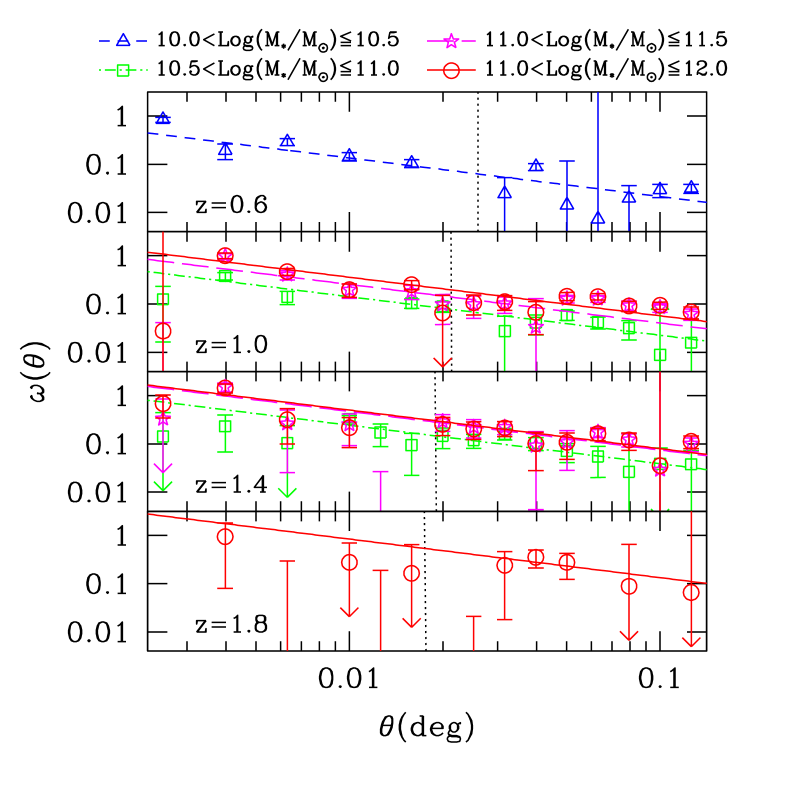
Figure 1: The 2-point angular correlation function as a function of redshift for our mass-selected samples in our field 3 (see text). The open triangle, open square, open star and open circle symbols represent the measurements made for the mass selected samples at stellar masses $10^{10.0}$$M_{\odot}\,$$<M_{*}\leq 10^{10.5}$$M_{\odot}\,$, $10^{10.5}$$M_{\odot}\,$$<M_{*}\leq 10^{11.0}$$M_{\odot}\,$, $10^{11.0}$$M_{\odot}\,$$<M_{*}\leq 10^{11.5}$$M_{\odot}\,$and $10^{11.0}$$M_{\odot}\,$$<M_{*}\leq 10^{12.0}$$M_{\odot}\,$, respectively. The best fitted lines for the correlation function are represented by the short-dashed, dashed-dotted long-dashed and continuous lines, respectively for the different mass samples as described above. The vertical dotted line corresponds to the lower limit at $\sim 1$$h^{-1}$Mpc of the range over which our data are fitted, in order to avoid any excess of pairs due to multiple halo occupation.

3 Clustering properties of massive galaxies

3.1 Angular clustering

The primary goal of this work is to study the clustering properties of galaxies selected according to their stellar mass. A clustering analysis is a study of the distribution of galaxies at all scales. Given its peculiar geometry, the EGS field is not ideally suited for such a study. Indeed, as galaxies are distributed along a strip in the EGS, the clustering properties at the largest scales are difficult to establish given the small numbers of objects we have in each stellar mass and redshift bin in this field. For the other three fields we mask out overlap regions, and other regions which do not have reliable photometry. This masking of regions empty of galaxies is then taken into account in the following analysis. Overall we performed our analyses over a total area of 0.7 deg².

Within our clustering analysis we first measure the 2-point angular correlation function $\omega(\theta)$ for our sample using the Landy & Szalay (1993) estimator:

$$\omega(\theta)={\mbox{DD}-2\mbox{DR}+\mbox{RR}\over\mbox{RR}}$$ (1)

where the DD, DR and RR terms refer to the number of data-data, data-random and random-random galaxy pairs having angular separations between $\theta$ and $\theta+\delta\theta$. Figure 1 shows the correlation function derived from our mass-selected samples in different redshift bins for one of our fields.

The best fit for the angular correlation is assumed to be a power-law of the form (Groth & Peebles, 1977):

$$\omega(\theta)=A_{\omega}(\theta^{-\delta}-C_{\delta})$$ (2)

with $A_{\omega}$ the amplitude at 1 degree, $\delta$ the slope, and $C_{\delta}$ the integral constraint due to the limited area of the survey. For statistical reasons we fix the slope to the commonly used fiducial value of $\delta=0.8$ (Groth & Peebles, 1977). We also estimate the integral constraint ($C_{\delta}$) as follows (Roche et al., 1993),

$$C_{\delta}={1\over{\Omega^{2}}}\int\!\int\theta^{-\delta}d\Omega_{1}d\Omega_{2}$$ (3)

where $\Omega$ is the area subtended by the survey field. To determine $C_{\delta}$ we numerically integrate this expression over each field, excluding masked regions. Assuming a slope of $\delta=0.8$, the unmasked areas ($S_{F}$) covered by the fields, and the corresponding integral constraint values are: $S_{F2}=639.55$ arcmin² and $C_{0.8\,F2}=3.61$, $S_{F3}=777.30$ arcmin² and $C_{0.8\,F3}=3.76$, $S_{F4}=731.04$ arcmin² and $C_{0.8\,F4}=3.69$, for fields 2, 3 and 4 respectively.

In order to fit the clustering reliably, we avoid the small-scale excesses due to possible multiple galaxy occupation of a single dark matter halo, as has been shown to exist in recent studies (e.g. Ouchi et al., 2005). The lower bound on which we fit our correlation was chosen to correspond to $\sim 1$$h^{-1}$Mpc , the observed one-halo term limit established by Zehavi et al. (2004). These lower bounds are shown by the vertical dotted lines on Figure 1, and it is worth noting that no apparent excess is displayed at the smallest scales.

The error-bars shown on Figure 1 are estimated from a jackknife Monte-Carlo method. The error estimation for each scale is made following the bootstrap method. In each sub-sample, objects are randomly removed and duplicated from our position catalogue, and the two-point correlation function is measured again. The value of the correlation function at each scale is estimated from the mean of these bootstrap catalogues, and errors are derived from the variance. We then derive the best fit amplitude for each of our fields at 1 degree using a Marquardt least-linear method, that take into account our bootstrap errors, and provide an estimate of the error on the fitting. We then derive a mean value from our six catalogues and over each of our three fields. Table 2 summarises the values measured for our samples.

As explained in Section 2.2.3, the variance over the six catalogues is used as an estimate for the systematic errors in the photometric redshift determination and the variance over the three field measurements is used as an estimate of the cosmic variance of our samples. Our total error budget is a quadratic sum of the fitting errors, photometric redshift errors, and cosmic variance errors. As discussed in Conselice et al. (2007), using models from Somerville et al. (2004), the cosmic variance on the number counts in the redshift range we use ($0.4<z\leq 2.0$) range from $\sigma_{v}\sim 0.1-0.2$ for our less massive samples, up to $\sigma_{v}\sim 0.3-0.5$ for our most massive ones. This is comparable with the uncertainties we derived based on our field-to-field measurements on the clustering analysis.

Figure 2: (a) Correlation length ($r_{0}$) as a function of redshift. The correlation lengths measured for our different samples are represented by the full circles with the size of the circle increasing with the stellar mass of the samples. We also show measurements performed by Meneux et al. (2008) for two mass ranges (Log $[M_{*}/(h_{100}^{-2}M_{\odot})]=10.22$ and $10.70$). The lines represent predictions from models by Mo & White (2002) for different minimum masses of dark matter haloes (plain lines for $M_{\rm min}=10^{11.0}$$h^{-1}M_{\odot}\,$, $10^{12.0}$$h^{-1}M_{\odot}\,$and $10^{13.0}$$h^{-1}M_{\odot}\,$, and dashed lines for $M_{\rm min}=5\times 10^{11.0}$$h^{-1}M_{\odot}\,$, $5\times 10^{12.0}$$h^{-1}M_{\odot}\,$and $5\times 10^{13.0}$$h^{-1}M_{\odot}\,$) while the dotted lines represent the predictions from models including halo distributions as described in Zheng et al. (2007). (b) Abundance ($n$) as a function of redshift. The abundances measured for our different samples are represented by the full circles with the size of the circle increasing with the mass of the sample. The lines represent predictions from models by Mo & White (2002) and Zheng et al. (2007) for different minimum masses of dark matter haloes (as described above).

Despite the accuracy of our photometric redshifts, as described in Section 2.2.3, our samples, selected in different redshift bins, are possibly contaminated by galaxies at other redshifts. Any contamination will dilute the original clustering signal, and therefore our measurements of the amplitude of the correlation function could be underestimated. From our Monte-Carlo simulations, we estimate the maximum contamination at a level from 20% to 30%, mainly due to galaxies from adjacent lower redshift bins (see Section 2.2.3 for a full description of this). This contamination is stronger at higher redshifts. However, this effect does not significantly alter our results. In the worst case, if the contaminating population is uncorrelated, the value of $A_{\omega}$ is diluted by a factor of $1/(1-f)^{2}$ (with $f$ the contamination fraction), corresponding to an underestimation of our correlation amplitude by a factor between 1.56 and 2.04 (for 20% and 30% contamination by other redshift galaxies). These factors are upper limits, and the true value of $A_{\omega}$ is likely to remain within the error-bars quoted in Table 2. In any case, this contamination will only reduce the strength of the clustering, and again our measures are therefore at worst lower limits. This means that any errors in redshifts and/or stellar masses only dilute our signal, which would make the real clustering strengths even higher than the ones we observe. Furthermore such an effect is included in our error budget as we are taking the average of measurements over six catalogues with perturbed redshift distributions, as described in Section 2.2.3. This method should account for the errors due to interlopers.

Moreover, our samples, divided into different stellar mass bins, are also subject to possible contamination from other stellar mass bins. Given the mass uncertainties of 0.2-0.3 dex (see Section 2.2.2), it is possible that galaxies more or less massive, and therefore more or less clustered, contaminate our stellar mass cuts. As mentioned in the Section 2.2.3, these effects are more difficult to constrain with our Monte-Carlo simulations. However within a given redshift bin, the measurements of the clustering for samples in adjacent stellar mass bins are very similar and overlap within their errorbars. The cross-contamination would therefore only have a minor impact, and in the sense of increasing the segregation.

3.2 Spatial correlation lengths and bias

In order to compare the clustering of galaxy populations at different redshifts we derive the spatial correlations for our galaxy samples. We do this by using the spatial correlation function ($\xi$) (Groth & Peebles, 1977) to derive $r_{0}$, the co-moving galaxy correlation length, as defined by:

$$\xi(r,z)=\left({\frac{r}{r_{0}(z)}}\right)^{-\gamma}$$ (4)

where $\gamma=1+\delta$. The redshift dependence is included in the co-moving correlation length $r_{0}(z)$. In general the larger the correlation length ($r_{0}$), the more clustered the galaxies are.

By measuring the redshift distribution for our samples we can also derive the correlation length $r_{0}$ from the amplitude of the angular correlation $A_{\omega}$ using the relativistic Limber equation (Magliocchetti & Maddox, 1999). We estimate correlation lengths assuming that our galaxies are distributed as Top-Hat functions in each of our narrow redshift bins. Given the derived statistics of our samples and the narrow redshift bins we are using here, and despite the accuracy of our photometric redshifts, changing the shape of the redshift distribution has a negligible impact on the results.

z bin(a)	$M_{*}$ bin(b)	$<z>$(c)	$<M_{*}>$(d)	$N^{(e)}$	$n$(f)	$A_{\omega}$(g)	$r_{0}$(h)	$b$(i)
					$\times 10^{-4}$	$\times 10^{-3}$
0.4–0.8	10.0–10.5	$0.61\pm 0.12$	$10.28^{+0.12}_{-0.17}$	$0.91\pm 0.17$	$35.9\pm 8.1$	$3.8\pm 1.9$	$5.7\pm 1.5$	$1.1\pm 0.3$
0.8–1.2	10.5–11.0	$0.99\pm 0.12$	$10.77^{+0.12}_{-0.17}$	$1.12\pm 0.11$	$25.1\pm 3.1$	$3.3\pm 1.0$	$5.6\pm 1.0$	$1.3\pm 0.2$
–	11.0–11.5	$0.98\pm 0.11$	$11.19^{+0.12}_{-0.16}$	$0.53\pm 0.04$	$11.9\pm 1.1$	$6.6\pm 2.6$	$8.2\pm 1.8$	$1.8\pm 0.4$
–	11.0–12.0	$0.98\pm 0.11$	$11.23^{+0.16}_{-0.23}$	$0.56\pm 0.04$	$12.5\pm 1.0$	$7.2\pm 2.2$	$8.6\pm 1.4$	$1.9\pm 0.3$
1.2–1.6	10.5–11.0	$1.37\pm 0.12$	$10.75^{+0.13}_{-0.18}$	$0.47\pm 0.11$	$8.2\pm 2.3$	$6.1\pm 2.1$	$7.7\pm 1.5$	$2.0\pm 0.4$
–	11.0–11.5	$1.38\pm 0.12$	$11.20^{+0.12}_{-0.17}$	$0.23\pm 0.05$	$4.0\pm 1.0$	$11.8\pm 4.9$	$11.1\pm 2.6$	$2.8\pm 0.6$
–	11.0–12.0	$1.38\pm 0.12$	$11.25^{+0.16}_{-0.25}$	$0.25\pm 0.05$	$4.3\pm 1.1$	$11.5\pm 5.4$	$10.9\pm 3.0$	$2.8\pm 0.7$
1.6–2.0	11.0–12.0	$1.73\pm 0.09$	$11.28^{+0.18}_{-0.28}$	$0.11\pm 0.04$	$1.7\pm 0.7$	$24.0\pm 18.5$	$15.2\pm 6.5$	$4.2\pm 1.6$

^(a)Redshift bin; ^(b)Stellar mass bin in Log$(M/M_{\odot})$; ^(c)Mean redshift; ^(d)Mean stellar mass in Log$(M/M_{\odot})$; ^(e)Density in arcmin^-2; ^(f)Abundance in $h^{3}$Mpc^-3; ^(g)Correlation amplitude at 1 degree; ^(h)Correlation length in $h^{-1}$Mpc ; ⁽ⁱ⁾Bias.

Table 2: Summary of the measurements performed for each sample of galaxies selected in redshift and stellar mass. The mean redshift, the mean stellar mass, surface density, space abundance, amplitude of clustering at 1 degree with a slope of $\delta=0.8$ (according to equation 2), the correlation length (according to equation 4), and the linear bias (according to equation 5) are compiled for each sample.

The correlation length is derived from the amplitude of the angular correlation function in each of our redshift and stellar mass bins, using each of the six catalogues (the original and the simulated versions) for each of our three fields. The mean correlation length is then computed, as well as its associated error budget, as described in Section 3.1. In summary, we find that correlation lengths vary from $5$$h^{-1}$Mpc to $15$$h^{-1}$Mpc for galaxies selected by stellar masses with $M_{*}>10^{10}$$M_{\odot}\,$. The highest correlation lengths are for the most massive galaxies at the highest redshifts $z=1.6-2$ (Figure 2(a)). In general, at lower stellar masses and redshifts, the correlation length becomes smaller.

Table 2 summarises the values we calculate for the correlation length $r_{0}$ measured within our stellar mass selected samples. In Figure 2 we plot the correlation length, and the galaxy number density, as a function of redshift for our stellar-mass-selected galaxy samples. We observe an apparent decrease in the correlation length with decreasing redshift, as is also observed in other previous studies (e.g. Le Fèvre et al., 2005). Here the main effect is the well-known luminosity-segregation, with brighter galaxies (less abundant) having a larger correlation length (Pollo et al., 2006; Coil et al., 2006). As a first rough approximation, this can be directly linked to a mass-segregation effect, with more massive galaxies more clustered. Previously, McCracken et al. (2008) showed that bright red galaxies, that are likely very massive, have clustering lengths that are almost invariant with redshift since $z\sim 1$, while less luminous (likely less massive) galaxies have correlation lengths that decrease with fainter magnitude at all redshifts.

As shown in Figure 2(a), we compare our results with Meneux et al. (2008), who have derived correlation lengths from spatial correlation functions using the VIMOS-VLT Deep Survey (VVDS) data-sets. The mean redshift of their sample is $\overline{z}\simeq 0.85$, and for galaxies with masses Log $[M_{*}/(h_{100}^{-2}M_{\odot})])=10.22$ they derived $r_{0}=5.06\pm 0.49$$h^{-1}$Mpc , and for galaxies with masses Log $[M_{*}/(h_{100}^{-2}M_{\odot})]=10.70$, $r_{0}=6.21\pm 0.67$$h^{-1}$Mpc . We note that these results are in good agreement within the error-bars of our measurements.

As analysed in Section 3.1 a contamination of our different samples by galaxies in adjacent redshift and stellar mass bins will artificially decrease the measured value of their correlation length. This effect is more likely to occur within the higher redshift samples, and thus the values summarised in Table 2 can be considered as lower limits of the real intrinsic correlation length. Such an effect has bin identified in previous analysis as well (e.g. Arnouts et al., 1999; Quadri et al., 2008). The net effect of this is that our estimates of the total masses for these galaxies are also lower limits. However, even with a contamination fraction at the upper limit of 20% and 30%, as quoted in Section 3.1, the values of the correlation lengths we quote in Table 2 are only under-estimated by a factor $\sim 1.28$ and $\sim 1.41$ respectively. The relative uncertainties on our measured correlation length are of the same order as this correction (Table 2). This is an upper limit of the correction that could be applied, and furthermore our correlation length measurements and errors take into account these potential effects from interlopers as described in Sections 2.2.3 and 3.1.

We also note that Hartley et al. (2008) have found that the errors on photometric redshifts can artificially broaden the redshift distribution which leads to an overestimate of the correlation length $r_{0}$. However given the narrow bins we are using in the current analyses, our redshift distributions are more perturbed by objects scattered from one redshift bin to another, than from a broadening effect due to photometric redshift errors.

In addition, we derive the linear bias of our sample, which relates the clustering of galaxies to that of the overall dark matter distribution (Magliocchetti et al., 2000). The rms density fluctuations of haloes ($\sigma_{8,\rm gal}(z)$) are linked to the rms density fluctuations of the underlying mass ($\sigma_{8,\rm m}(z)$) by the bias ($b(z)$) following:

$$b(z)=\frac{\sigma_{8,\rm gal}(z)}{\sigma_{8,\rm m}(z)}$$ (5)

where $\sigma_{8,m}(z)=\sigma_{8}D(z)$ is the variance in $8$$h^{-1}$Mpc spheres, assuming that dark matter behaves as predicted in linear theory (linear growth $D(z)$ - Carroll et al., 1992), renormalised to the fiducial value $\sigma_{8}$ (fixed to $\sigma_{8}=0.9$ in this study). If the galaxy correlation function is fit as a power law, then it can be integrated to give the relative variance in $8$$h^{-1}$Mpc spheres: $\sigma_{8,gal}$ (Peebles, 1980). We find for our sample that the bias varies from $b\sim 1.1$ to $b\sim 4.2$ for galaxies selected by stellar masses $M_{*}>10^{10}$$M_{\odot}\,$. The most massive galaxies at the highest redshifts $z=1.6-2$ are more biased, in good agreement with biased galaxy formation models (Bardeen et al., 1986). Table 2 summarises the values of the bias $b$ measured for our samples.

z bin(a)	$M_{*}$ bin(b)	$<z>$(c)	$<M_{*}>$(d)	$M_{\rm min-r_{0}}$(e)	$f_{r_{0}}$(f)	$M_{\rm min-n}$(g)	$f_{n}$(h)	$M_{\rm DM}$(i)	$M_{*}/M_{\rm DM}$(j)
									$\times 10^{-2}$
0.8–1.2	11.0–11.5	$0.98\pm 0.11$	$11.19^{+0.12}_{-0.16}$	$12.75^{+0.19}_{-0.36}$	$1.13$	$12.69^{+0.11}_{-0.15}$	$0.89$	$12.70^{+0.21}_{-0.43}$	$3.15\pm 2.21$
–	11.0–12.0	$0.98\pm 0.11$	$11.23^{+0.16}_{-0.23}$	$12.85^{+0.15}_{-0.24}$	$1.10$	$12.67^{+0.10}_{-0.13}$	$0.90$	$12.80^{+0.17}_{-0.27}$	$2.63\pm 1.69$
1.2–1.6	10.5–11.0	$1.37\pm 0.12$	$10.75^{+0.13}_{-0.18}$	$12.55^{+0.18}_{-0.30}$	$1.16$	$12.76^{+0.11}_{-0.16}$	$0.92$	$12.49^{+0.19}_{-0.35}$	$1.85\pm 1.21$
–	11.0–11.5	$1.38\pm 0.12$	$11.20^{+0.12}_{-0.17}$	$13.18^{+0.18}_{-0.32}$	$1.04$	$12.98^{+0.12}_{-0.17}$	$0.94$	$13.17^{+0.19}_{-0.34}$	$1.08\pm 0.69$
–	11.0–12.0	$1.38\pm 0.12$	$11.25^{+0.16}_{-0.25}$	$13.16^{+0.21}_{-0.41}$	$1.05$	$12.96^{+0.12}_{-0.18}$	$0.92$	$13.14^{+0.21}_{-0.44}$	$1.29\pm 1.01$
1.6–2.0	11.0–12.0	$1.73\pm 0.09$	$11.28^{+0.18}_{-0.28}$	$13.50^{+0.26}_{-0.74}$	$1.02$	$13.14^{+0.13}_{-0.20}$	$0.96$	$13.50^{+0.26}_{-0.79}$	$0.61\pm 0.60$

^(a)Redshift bin; ^(b)Stellar mass bin in Log$(M/M_{\odot})$; ^(c)Mean redshift; ^(d)Mean stellar mass in Log$(M/M_{\odot})$; ^(e)Minimum mass of the Dark Matter Halo estimated from the correlation length in Log$[M/(h^{-1}M_{\odot})]$; ^(f)Correction factor for accounting of the halo distribution effect (estimated from correlation length); ^(g)Minimum mass of the Dark Matter Halo estimated from the correlation length in Log$[M/(h^{-1}M_{\odot})]$; ^(h)Correction factor for accounting of the halo distribution effect (estimated from abundance); ⁽ⁱ⁾Mass of the Dark Matter Halo as estimated from the correlation length and after correction for the halo occupation in Log$[M/(h^{-1}M_{\odot})]$; ^(j)Stellar-mass-to-Dark-Matter-mass ratio in units of $h$.

Table 3: Summary of the measurements performed for each sample of galaxies selected in redshift and stellar mass. The mean redshift, the mean stellar mass, the minimum masses of associated DMHs as inferred by the comparison between the DMH model and the correlation length,the DMH model and the abundances, and the correction factor to apply to take into account the halo distribution effect are compiled for each sample. In addition we add the value we use as the mass of the DMH and the stellar-mass-to-dark-matter-mass ratio, as inferred by the correlation measurements, and corrected for the halo occupation effect.

4 Total dark matter mass of massive galaxies at z $\mathbf{<2}$

4.1 Modelling the dark matter halo correlation lengths and abundances

The standard CDM model predicts that at any redshift more massive dark matter haloes are on average more clustered than lower mass systems. To model this effect quantitatively, we use the predicted effective bias, and the abundance evolution, as derived from the Mo & White (2002) formalism for different minimum dark matter halo (DMH) mass thresholds. This formalism is based on modelling the effective bias, which relates the mass fluctuations of haloes, to the mass fluctuations in spheres that contain an average mass $M$ of underlying dark matter, according to equation 5. For this purpose, we use the halo abundance distribution as a function of mass and redshift determined by Sheth & Tormen (1999), derived from fits to large N-body simulations, and the linear halo bias for a given mass at a given redshift, calculated using the function of Sheth et al. (2001). We directly derive the effective bias by integrating the ratio of these functions on masses above a given minimum mass $M_{\rm min}$.

A modelling of the correlation length evolution for DMHs of a given minimum mass $M_{\rm min}$ at a given redshift $z$ can be directly derived from the effective bias using the recipes described in Magliocchetti et al. (2000). We use also these recipes in the computation of the linear bias for our sample of galaxies, as described in Section 3.2. Details of this method can be found in the cited papers. The predicted correlation lengths and abundances evolutions as a function of redshift are shown in Figures 2(a) and (b), for different values of the minimum mass of DMHs, $M_{\rm min}$.

We note that this model assumes that there is only one galaxy per DMH. Such an assumption can and often must be incorrect, especially in the case of the less massive galaxies in the lowest redshift bins. If satellite galaxies are taken into account, using the same galaxy bias factor measured from the data, a different $M_{\rm min}$ would be inferred. In order to take into account the Halo Occupation Distribution (HOD) effect we follow the simple recipe provided in Zheng et al. (2007), by summing a step function for central galaxies and a power law for satellite galaxies, $\langle N(M)\rangle=1+M/M_{1}$ for $M>M_{\rm min}$. As inferred in Zheng et al. (2007), and following galaxy formation model predictions (e.g. Zheng et al., 2005) and HOD modelling results (e.g. Zehavi et al., 2005), we use $M_{1}=20M_{\rm min}$. The modified correlation lengths and abundance evolutions are shown in Figures 2(a) and (b) with dotted lines, for different values of the minimum mass $M_{\rm min}$.

4.2 Dark matter masses of massive galaxies

In Figures 2(a) and (b) we show the predicted relation, based on dark matter halo models and on Halo Occupation Distribution, between the correlation lengths and the number densities of dark matter haloes, and how this relation evolves with redshift. These predictions are in good agreement with our observations. As expected, the mass segregation effect is present, with the correlation lengths derived for galaxies with higher stellar mass agreeing well with the predicted correlation lengths of haloes with the highest dark matter masses.

We go a step further than this and associate the observed correlation lengths of our stellar mass selected samples with the predicted value of their host halo masses, thereby providing an estimate of the typical halo mass for each stellar mass selected bin. To do this, we make the assumption that only one galaxy is hosted per halo. Later we apply a correction to take into account the halo occupation effect. Finally, we investigate the stellar masses of all galaxies within these haloes to obtain a measurement of the total stellar to halo mass within dark matter haloes.

This total mass measurement from our clustering analysis gives us a measure of how massive the haloes that host massive galaxies are. To obtain these mass measures, we interpolate masses from a grid of predictions in correlation length/redshift space, from the models described in Section 4.1. Each observed correlation length at a given redshift is then assigned to a model with a given DMH minimum mass. This method has been used previously in papers such as Ouchi et al. (2004); Magliocchetti et al. (2008); Yoshida et al. (2008). The errors on the correlation lengths are propagated to obtain errors on the DMH minimum mass in the same way. A similar approach is used to estimate the mass of DMHs, by comparing model results with the abundances. Table 3 summarises the values derived for the DMH minimum mass $M_{\rm min}$ from their correlation length values and from their abundances.

Our assumption of a single galaxy per halo can result in overestimating the true value of the DMH minimum mass. Following Zheng et al. (2007), we estimate the effect of halo occupation using a simple prediction described in Section 4.1. However as shown by Zheng et al. (2007), the effect of the “one galaxy per halo” assumption on the true measure of the DMH mass can be very important at the lower bias levels found in the lower redshift part of our catalogue. The simple correction we apply is unlikely to be sufficient to correct for this effect, so we later discard these sub-samples from our following analysis, as shown in Table 3.

More detailed models, such as HOD models (e.g. Wechsler et al., 2001; Zehavi et al., 2005), are likely more appropriate to determine the mass of DMHs associated with a sample of galaxies. For instance, in order to have a reliable estimate of the mass of the DMHs, such halo occupation models should fit directly from the angular correlation function determined for the samples in the lower redshift and stellar masses bins. However, for our higher redshift samples with a strong bias, we have estimated our correlation amplitude on scales $>1$$h^{-1}$Mpc , where the effects of any extra halo terms is avoided (see Section 3.1). Zehavi et al. (2004) have shown that one-halo term clustering is only observable on scales smaller than this limit. Therefore, our lower mass galaxies likely reside in the same haloes, but our measurements are made on scales where galaxies are in separate haloes. This should reduce the effect of multiple halo occupation on our estimation of the DMH mass even for the lower mass samples. One advantage in measuring clustering over large areas, such as in this study, is the ability to avoid the one-halo clustering regime, unlike in previous studies using smaller areas.

As shown in Figures 2(a) and (b), the minimum mass of dark matter haloes, for a given sample of galaxies, can differ when estimated from the correlation length measurements or through using abundance measurements. Magliocchetti et al. (2008) raised a similar issue in their analyses, and showed that this discrepancy could also come from an erroneous a priori assumption of the one-parameter halo bias model for a one-to-one correspondence between dark matter haloes and astrophysical sources. When we correct for this effect the two estimations are broadly in agreement. The masses of DMHs derived from the comparisons between the DMH model (without halo occupation effects corrected) and the correlation lengths and abundances are summarised in the Table 3.

Figure 3 shows the mass of DMH inferred by the abundance measurements compared with the one inferred by the correlation length measurements, with both quantities corrected to account for halo distribution effects. The mild residual discrepancy between the masses estimated by comparing the models with the correlation length or the abundances, can be explained by several, likely combined, effects.

First, and most likely, the contamination effects between the different bins of our sample could be at the origin of the discrepancy seen in Figure 3. As seen in Section 3.2, the correlation lengths we are using here are lower limits, due to possible contamination of the samples by interlopers. Therefore the masses of the DMHs we measure from the correlation lengths are also lower limits. However, this is what we want as the models provide the minimum mass of the DMHs, and using the lower-limits is consistent with this. Also, interlopers will affect the measurements of the abundances of our different samples. It is more likely that we are overestimating the number of objects in our less populated samples, which are the more massive systems. In this case, the masses of DMHs derived from the abundances of our most massive stellar samples are likely underestimated. The combination of these two effects is likely the origin of the discrepancy between our two estimates, as shown in Figure 3. These contamination effects are included in our error budget as we discuss in Section 3.2, and, given the difficulty in obtaining a precise evaluation of the contamination, we do not correct our measurements directly for these effects.

A second possible explanation, would be incorrect redshift distributions for our samples. Quadri et al. (2008) found a similar discrepancy between the clustering and the abundance of their colour selected sample, and invoked an incorrect redshift distribution as a likely origin of such discrepancy. In our case as we are using simple Top-Hat functions, given the narrow size of our redshift bins, this effect relates directly to the contamination.

Furthermore, Tinker et al. (2010) claim that such a discrepancy could originate from cosmic variance and incorrect models of the halo mass function and halo bias function. In our case, we take into account cosmic variance in our error budget, through the field-to-field variance, so we can partially reject this explanation. Finally, our models may be incorrect, despite being extensively tested. We recompute the model using a slightly modified halo bias function from the original function of Sheth et al. (2001), as proposed by Tinker et al. (2005). By changing the halo bias function we only modify the masses estimated from the correlation lengths. As shown in Figure 3, the masses inferred by this new model are not in better agreement, and the measurements remain almost within our original errorbars. We decided to keep the measurements made using the Sheth et al. (2001) function, as it is more commonly used. However other inputs in our models, such as the halo mass function, may also be at the origin of the discrepancy.

Gao et al. (2005) have also shown that the clustering of DMHs depends not only on their halo mass but also on their assembly history, and especially on their formation time. This “Halo Assembly bias” implies that, at a given mass, DMHs which assembled earlier are more clustered than DMHs that assembled later. This effect will increase the discrepancy between masses measured from the correlation length matching, and from the abundance matching. Croton et al. (2007a) have shown that the bias induced by the environmental dependence of halo formation history at a fixed halo mass is stronger for faint red central galaxies and weaker for bright red galaxies. The assembly bias enhances the two-point correlation by $\sim 10\%$ for bright galaxies, and suppresses it by the same amount for fainter galaxies. However the relative strength in clustering between our more massive and less massive samples is $\sim 40\%$, much higher than the effect of the assembly bias itself. Furthermore, Gao et al. (2005) report that this effect is weakest for DMHs with masses $M_{\rm DM}>10^{13}$$h^{-1}M_{\odot}\,$which are within our range.

The masses of the DMHs calculated by matching correlation lengths and abundances to the models both suffer from uncertainties. However as shown in Figure 3, the two estimates are broadly in agreement within our errorbars. We decided therefore to use the mass estimated from the correlation lengths corrected from the HOD effect, as we have a more complete error budget in this case.

Figure 3: Comparison between the masses of DMHs, as estimated using correlation lengths (r₀) and abundances (n). The masses are corrected from the Halo Distribution effects. The plain symbol represent the masses estimated from the model using the halo bias function from Sheth et al. (2001), and the dotted symbols from the model using the halo bias function from Tinker et al. (2005).

5 The Ratio of stellar and dark matter mass for massive galaxies between $\mathbf{0<}$ z $\mathbf{<2}$

5.1 History of mass assembly of galaxies in massive DMHs

5.1.1 Stellar mass fraction in the central galaxy

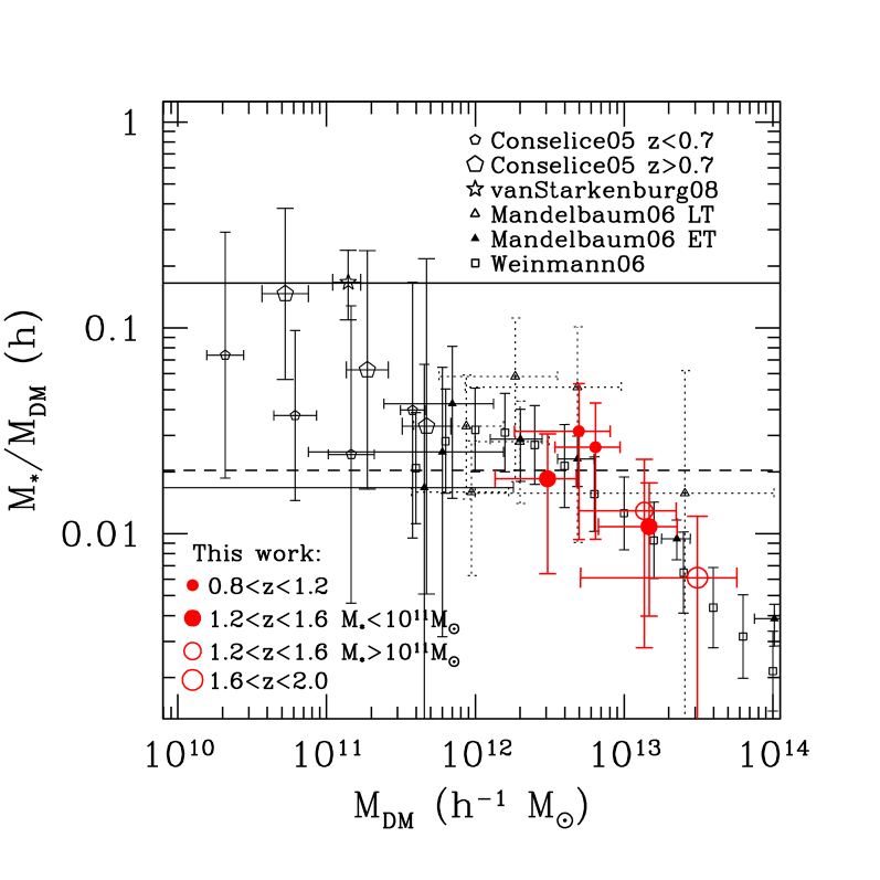
Figure 4: Evolution of the stellar mass fraction for massive galaxies as a function of the dark matter halo mass ($M_{\rm DM}$). The measurements made for this study are shown as red open and filled circles, with bigger size symbols corresponding to higher redshift samples. Different measurements taken from the literature are overplotted, with the size of the symbol bigger for samples with $z>0.7$. The continuous line represents the baryonic fraction measured from WMAP5 (Komatsu et al., 2009), and the dashed line represent the mean stellar fraction in the local Universe estimated by Cole et al. (2001).

Since we know the median stellar mass within each of our sample cuts, and the clustering and hence total masses of these same galaxies, we derive directly the stellar mass fraction as a function of total mass, and as a function of redshift for our sample. We report these values in Table 3, and display the results on Figures 4 and 5.

In order to study the link between luminous and dark matter we make several assumptions. First we assume that the minimum mass of the DMHs, determined as explained in Section 4.2, is an accurate approximation of the median mass of these DMHs ($M_{\rm min}\simeq M_{\rm DM}$). As we are mainly studying DMHs with masses $M_{\rm DM}>10^{12}$$h^{-1}M_{\odot}\,$, and the mass function of DMHs drops rapidly above this limit, we conclude that this assumption is fair (Warren et al., 2006). Our second assumption, for comparison to other work, is that the virial mass of a system is equivalent to the total mass in the DMH, which has been confirmed by Busha et al. (2005) using a large N-body simulation. The third assumption we make, in order to compare our measurements with literature values, is that the mass in dark matter is equivalent to the total mass of the system. Indeed, the Mo & White (2002) models we use to estimate the mass of the DMHs are based on the behaviour of dark matter, and do not take into account presence of baryonic matter. Given that baryonic matter accounts for $\lesssim 15\%$ of the total density in the Universe (Komatsu et al., 2009), this last assumption is justified, as $\gtrsim 85\%$ of the density of the system is made up of dark matter.

As explained in Section 4.2, we corrected our halo masses for multi-occupation of the haloes. We also focus our analysis on the highly biased samples, those most likely to have a one-to-one correspondence between the galaxy and its DMH, sans any outer satellite galaxies, which is an issue we address later. We can therefore assume that we are looking at the stellar mass fraction of the central galaxies, and are mostly free of any effect due to satellite galaxies in the present analysis.

To compare our results to previous work, we collected measurements of stellar and total masses from the literature based on various different methods to estimate the masses of various DMHs. These include total masses of disk-like galaxies based on rotation curves at $0.2<z<1.0$, from Conselice et al. (2005b), as well as at $z\sim 2.0$, from van Starkenburg et al. (2008). The stellar masses used in these studies are estimated from SED fits based on spectroscopically confirmed redshifts, and a wide range of photometry, similar to that described in Section 2.2.2, but by using a Salpeter IMF. We converted all stellar masses into a Chabrier IMF by dividing by a factor of $\sim 1.5$ (Chabrier, 2003).

We also added measurements of nearby early-type (ET) and late-type (LT) galaxies from galaxy-galaxy lensing studies in the Sloan Digital Sky Survey (SDSS) from Mandelbaum et al. (2006). Stellar masses for these SDSS galaxies are obtained from the method described in Kauffmann et al. (2003), based on the strength of the $4000$Å-break and the Balmer absorption index H$\delta_{A}$, for a Kroupa (2001) IMF (which give estimates very close to the Chabrier (2003) IMF). Finally, we use the publicly available catalogue of groups in the SDSS from Weinmann et al. (2006) to estimate the mass ratio for galaxy groups in the local Universe. Total masses of these groups are determined by ranking the completeness-corrected group luminosity, and by assigning to them the mass of the DMHs, ranked according to their abundances predicted by models from Mo & White (2002). The central galaxies of each group are assumed to be the most luminous galaxy in the group. The stellar masses for this sample are determined using the method described in Kauffmann et al. (2003).

We add as a continuous line on Figures 4 and 5 the value of the mean baryonic fraction in the Universe, estimated from WMAP5 (Komatsu et al., 2009), which is $f_{b}=\Omega_{b}/\Omega_{m}=0.165\pm 0.004$. From a study of galaxies in the local Universe, Cole et al. (2001) measure the stellar mass density to be $\Omega_{*}h_{100}=(2.9\pm 0.43)\times 10^{-3}$ for a Salpeter IMF. If we scale this value to a Chabrier (2003) IMF, and combine it with the cosmological parameters from WMAP5 (Komatsu et al., 2009), we derive a mean stellar mass fraction in the Universe of $f_{*}=(2.03\pm 0.04)\times 10^{-2}$, which is shown in Figures 4 and 5 as a dashed line. The remaining part of the baryonic fraction that is not included in stars is possibly present in the form of hot and warm gas, as seen in clusters (e.g. Arnaud & Evrard, 1999).

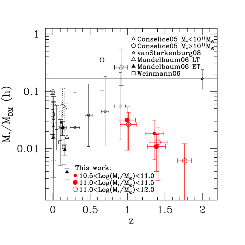
Figure 5: Evolution of the stellar mass fraction of massive galaxies as a function of redshift. The measurements made in this study are shown as red open and filled circles, with bigger sized symbols corresponding to more massive samples. Measurements taken from the literature are overplotted, with larger symbols for samples with $M_{*}>10^{11}$$M_{\odot}\,$. The lines representing the baryonic mass fraction and the local stellar mass fraction are the same as described in Figure 4.

Figure 4 shows that there is a good agreement between these very different mass measurements, especially at the massive end. The $M_{*}/M_{\rm DM}$ ratio, even when estimated from completely different methods, shows a clear decrease at higher halo masses in all studies. However, estimating accurate DMH masses is difficult, especially in the less massive cases. Dynamical estimates (rotation curves, e.g. Sofue & Rubin (2001); velocity dispersions, e.g. Balogh et al. (2007)) trace the innermost region of the galaxy, requiring extrapolation to estimate the total mass of the system. Weak-lensing requires the use of stacking methods to provide an accurate estimate of the total mass, and tend to be difficult to achieve in the case of less massive DMHs (e.g. Hoekstra et al., 2001; Mandelbaum et al., 2006). In our case, galaxies in less massive dark matter haloes are not strongly biased, making the assumption of a one-to-one correspondence between the galaxy and the DMH less appropriate, as mentioned earlier. However our method, based on clustering properties at large scales, is efficient enough to determine the luminous-to-dark matter mass ratio for massive galaxies, and has the advantage of allowing us to estimate masses at higher redshifts, where for instance lensing cannot be used.

Overall, we find that more massive systems have a lower ratio of stellar-to-halo-mass, as shown in Figure 4. This behaviour is seen in all of our measurements at $1.0<z<2.0$, as well as in the local Universe with the SDSS, and thus appears to be independent of redshift, and is perhaps universal. This relation implies that, at fixed total mass, the relationship between the mass of the central galaxy and its DMH does not evolve strongly with cosmic time. Physically this may imply that very massive galaxies struggle to increase their stellar mass in very clustered environments, resulting in a departure in the luminous-to-dark-matter mass ratio in massive DMHs compared to lower mass DMHs, which is below the average value in the local Universe. These observations also imply that there is a limit to how much stellar mass a galaxy can have, with a cut off at a few times $10^{11}$$M_{\odot}\,$. This is consistent with the observed cut-off at high mass of the stellar mass function at low redshift (e.g. Baldry et al., 2008).

Furthermore, a decreasing stellar mass fraction with increasing halo mass has been observed in groups and clusters (e.g. Eke et al., 2004; Lin & Mohr, 2004; Gonzalez et al., 2007; Balogh et al., 2007). Lin & Mohr (2004) show that Brightest Cluster Galaxies (BCGs) contribute a large fraction to the total light of their host cluster, but become progressively less important in the overall luminosity budget in the highest mass clusters. This effect is explained by differential growth between the BCGs and their host clusters, due to clusters accreting nearby galaxies in lower mass groups, while the BCGs grow modestly by merging or cannibalism (Whiley et al., 2008). Similarly we can imagine that the clusters will accrete more dark matter in a similar process while the central galaxy grows more slowly.

5.1.2 The stellar mass fraction in satellite galaxies

In Section 5.1.1 we focussed our analysis on the central galaxy of the DMH. Indeed, as explained in Section 4.2, our clustering measurements are made in a way where we can assume there is only one massive galaxy per DMH, from which we measure the mass of the host halo. However, an overabundance of satellite galaxies has been observed in massive DMHs (e.g. van den Bosch et al., 2005; Yang et al., 2005). It is therefore possible that a non-negligible fraction of the stellar mass in the most massive DMHs resides in satellite galaxies (e.g. Lin & Mohr, 2004; Balogh et al., 2008).

To study this possibility in more detail we use the SDSS group catalogue (Weinmann et al., 2006), as it provides stellar masses for each member of each group. We limit our analysis of these groups to those at $z<0.06$ in order to be complete at stellar masses $M_{*}>10^{10.0}$$M_{\odot}\,$, and at $z<0.045$ for $M_{*}>10^{9.5}$$M_{\odot}\,$. We plot the ratio of the total stellar mass in the SDSS group DMHs to the total mass of the DMHs in Figure 6. As shown in this figure, the limited completeness of the sample does not allow us to conclude if the mass in satellite galaxies can account for the totality of the “missing” stellar mass in the DMH. However, the stellar mass distribution of satellite galaxies in the SDSS, hosted by groups with DMHs masses of $10^{13.0}$$h^{-1}M_{\odot}\,$$<M_{\rm DM}<10^{13.5}$$h^{-1}M_{\odot}\,$, is shown in Figure 7. This study is limited to $z<0.06$, and shows a plateau before reaching the completeness limit of $M_{*}>10^{10.0}$$M_{\odot}\,$. This flattening at the faint end is similar to the observations of the luminosity function of the Local Group (e.g. Pritchet & van den Bergh, 1999).

Furthermore, a decrease in the stellar-mass fraction is also observed in local clusters. Vikhlinin et al. (2006) observed a deficiency of X-ray gas in galaxy groups compared to clusters. Gonzalez et al. (2007) explain these observations by the fact that the missing X-ray gas has cooled in less massive systems to form stars. This implies that a larger fraction of the baryonic matter in clusters is in the form of hot gas in more massive systems (e.g. Arnaud & Evrard, 1999). However, while the total mass can be derived from the virial mass for these massive clusters, the total stellar mass is harder to estimate. A non-negligible amount of the light emitted by a cluster resides in its Intracluster Light (ICL), as dynamical processes can strip stars from galaxies which orbit in the intracluster space (e.g. Lin & Mohr, 2004; Gonzalez et al., 2007, and references therein), making the estimate of the total stellar-mass in a cluster difficult to measure accurately.

In our study of the stellar-mass fraction from the SDSS group catalogue, given the likely incompleteness in establishing group membership, we can only conclude that there is a weak trend in which the stellar-mass fraction in more massive systems is lower than in less massive ones, as shown in Figure 6. Further study of the role of satellite galaxies in the total amount of stellar-mass in a DMH is required to fully understand this result.

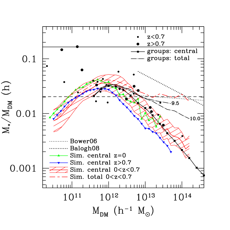
Figure 6: Evolution of the stellar mass fraction for massive galaxies as a function of dark matter mass ($M_{\rm DM}$). The values for our measurements, and previous values from the literature shown in Figure 4, are represented by the dots (small for $z<0.7$ and enlarged for $z>0.7$). The full squares connected by a full line represent the stellar fraction for the central galaxies in SDSS groups, and the long-dash-dotted lines represent the stellar fraction for all galaxies in SDSS groups at different completeness limits of $M_{*}=10^{10.0}$$M_{\odot}\,$and $M_{*}=10^{9.5}$$M_{\odot}\,$, corresponding to redshift limits of $z<0.06$ and $z<0.045$ respectively. The two thick straight dotted lines represent slopes of the evolution of the total stellar fraction (in central and satellite galaxies as well as in the ICL) with DMH masses as detailed in Balogh et al. (2008), and renormalised arbitrarily for more clarity, as we are only interested in comparing slopes. The green, red and blue lines represent the predictions from the De Lucia & Blaizot (2007) model for the central galaxies at different redshifts (resp. $z=0$, $0<z<0.7$ and $z>0.7$). The shaded red region represents the rms scatter of the predicted stellar mass fraction for the central galaxies at $0<z<0.7$. The red short-dash-long-dash line shows the prediction from the model for the total stellar mass fraction estimated from the De Lucia & Blaizot model. The horizontal continuous line represents the baryonic fraction measured from the WMAP5 analysis (Komatsu et al., 2009), and the horizontal dashed line represents the mean stellar fraction in the local Universe as measured by Cole et al. (2001).

5.1.3 “Halo downsizing”: a possible scenario for the formation of massive DMHs

Figure 5 shows that, at fixed stellar mass, the stellar mass fraction increases at lower redshift. In other words, the stellar component apparently grows more rapidly than the dark component between $1.0<z<2.0$ for galaxies with $M_{*}>10^{11.0}$$M_{\odot}\,$. However, as shown in Table 3, the average stellar mass in each stellar mass bin does not change significantly with cosmic time, while the average DMH mass decreases by a factor $\sim 5$ within these stellar mass selected samples. Furthermore, the star-formation rate does not change dramatically in the redshift range $1.0<z<2.0$ (e.g. Pérez-González et al., 2005; Tresse et al., 2007; Reddy et al., 2008), and the high-mass end of the stellar mass function does not evolve significantly below $z\sim 1-2$ (e.g. Drory et al., 2005; Bundy et al., 2006; Fontana et al., 2006; Pozzetti et al., 2007; Marchesini et al., 2009). This suggests that, instead of an increase of the average stellar mass, a statistical process is responsible for an apparent decrease of the average mass of massive DMHs between $z\sim 2.0$ and $z\sim 1.0$ for galaxies with stellar masses $M_{*}>10^{11.0}$$M_{\odot}\,$.

We propose that these observations for very massive galaxies ($M_{*}>10^{11.0}$$M_{\odot}\,$) can be explained by a “halo downsizing” effect (e.g. Neistein et al., 2006). We assume that the most massive galaxies are already in place at $z\sim 2$ in the most massive DMHs, in terms of their stellar material. Gradually the stellar mass bin we select is populated by galaxies that have gained stellar mass with time but that are hosted by less massive DMHs than the older systems we find at higher redshifts. Meanwhile the most massive galaxies do not gain in stellar-mass, nor in DMH mass, due to a quenching of their star formation and a weak merging rate (Drory & Alvarez, 2008). As a consequence the average mass of the DMHs for these galaxies decreases, and the stellar mass ratio increases, which is what we find.

Such an idea is supported by the “Archaeological downsizing” (Thomas et al., 2005), and the observation that the most massive galaxies appear to have assembled their stellar mass earlier than younger galaxies. Galaxies with $M_{*}>10^{11.5}$$M_{\odot}\,$assembled half of their stellar mass before $z\sim 1.5$, and more than 90% of their mass was already in place at $z\sim 0.6$ (Bundy et al., 2006; Pérez-González et al., 2008). Such observations imply that the mechanism responsible for quenching star-formation in galaxies is strongly mass-dependent and that it occurs earlier in the most massive galaxies (Bundy et al., 2006, 2008). Using semi-analytical models, Cattaneo et al. (2008) have shown that the downsizing effect observed for red galaxies, could naturally result from a shutdown in star-formation. More massive central galaxies in today’s Universe formed earlier and over a shorter period of time than less massive galaxies. A critical mass of DMHs of $M_{\rm DM}\sim 10^{12}$$h^{-1}M_{\odot}\,$, above which a shutdown in star-formation occurs, is also observed in these studies, corresponding roughly to the mass where we observe a decline in the stellar-to-dark-matter-mass-ratio in Figure 4.

As mentioned in Section 4.2, the “Assembly bias” effect could also mimic the observed increase of stellar-mass ratio with lower redshifts. Croton et al. (2007a) have shown that, at fixed halo mass, more massive and clustered central galaxies tend to occupy haloes that formed earlier, while less clustered central galaxies occupy haloes that formed later. However, Gao & White (2007) have demonstrated that this effect is unobservable for massive DMHs ($M_{\rm DM}\sim 10^{13}$$h^{-1}M_{\odot}\,$). Although we cannot rule out that assembly bias could artificially increase the ratio of stellar to dark matter mass which we observe, this effect is likely not large enough to account for the observed evolution.

The “halo downsizing” effect could also be used to explain the observation that galaxies in more massive haloes contain a lower stellar-mass fraction than those in less massive haloes, as seen in Figure 4. A tentative explanation of the formation of massive galaxies could be that at higher redshift the most massive DMHs formed rapidly by accretion or mergers (Conselice et al., 2003). This would provide galaxies less time to form stars and become more subject to a shutdown of their star-formation, compared with less massive DMHs (Bundy et al., 2006; Pérez-González et al., 2008). Moreover, the gas accreted in the more massive DMHs is hot, which cannot cool quickly in such massive potentials, suppressing further the star-formation in these massive galaxies, as observed for groups and clusters (Gonzalez et al., 2007).

The main difficulties in testing directly the scenario described above are in measuring accurately the stellar and dark matter masses involved. We assume within our clustering-derived masses, and through the other mass estimations, that masses of DMHs, dynamical masses, and total masses, are equivalent. However, it is not always easy to compare dynamical masses with the often used $M_{500}$ and $M_{200}$ masses, derived for a radius of a system corresponding to overdensities of 500 and 200, relative to the critical density at a given redshift. Furthermore, dynamical masses are extremely difficult to measure in low mass systems, particularly at high redshift. On the other hand, the total amount of stellar mass and gas mass in the most massive systems is also difficult to measure, and requires extensive observations. For instance, a deeper study in the near-infrared bands of local groups and clusters is required to obtain a better measure of the stellar mass fractions in the satellites galaxies and in the ICL. In addition, a better estimate of the gas content of clusters and groups, through very detailed X-ray studies of a large sample, would be extremely valuable.

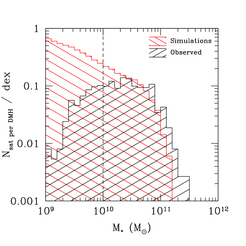
Figure 7: The distribution in stellar mass for satellites in DMHs of masses $10^{13.0}$$h^{-1}M_{\odot}\,$$<M_{\rm DM}<10^{13.5}$$h^{-1}M_{\odot}\,$. The histogram in black represents the distribution as observed in SDSS groups at $z<0.06$, and the histogram in red is the distribution in the Millennium simulation. The vertical dashed line represents the completeness limit in stellar mass of the SDSS at $z<0.06$.

5.2 Modelling the mass assembly of massive DMHs with semi-analytic models

5.2.1 Modelling the history of the central galaxy

Semi-analytic models are known to struggle in reproducing the observed formation of the most massive galaxies, pushing the formation of these systems to very late epochs (e.g. Kauffmann & Charlot, 1998; Conselice et al., 2007). By introducing AGN feedback (e.g. Springel et al., 2005a; Bower et al., 2006; Croton et al., 2006) the most recent models now manage to reproduce a star formation “downsizing” effect, implying that the stars in more massive galaxies form early in the Universe (De Lucia et al., 2006). In order to check if these models are able to reproduce the behaviour we observe between stellar mass fraction and total mass, how this fraction evolves with redshift, and to better understand the underlying physical processes involved, we compare our results to those from one of the current leading models. We use the Millennium simulations (Springel et al., 2005b) in which were implemented the semi-analytic models developed by De Lucia & Blaizot (2007).

The Millennium model predictions for the stellar mass fraction of the central galaxy of DMHs, at different redshifts ($z=0$, $0<z<0.7$, $z>0.7$), are shown in Figure 6, with the dashed area showing the rms for predicted DMHs at $0<z<0.7$. As expected, the peak in the mass ratio vs. halo mass occurs at $M_{\rm DM}\sim 10^{12}$$h^{-1}M_{\odot}\,$, where star formation is known to be the most efficient. In less massive DMHs the infall time of gas clouds is too long to form stars efficiently, while in more massive haloes it is the cooling time of the gas cloud that is too long (White & Frenk, 1991). By construction, the mean value of this ratio in the models is similar to the observed stellar-mass fraction in the local Universe. The model from De Lucia & Blaizot reproduces well the behaviour observed for the central galaxies in the most massive DMHs at low redshifts. However, at higher redshifts the agreement is not as good, with the model showing lower stellar mass fractions compared to our observations. These models seem to not form massive galaxies quickly enough to reproduce the observations (see also Conselice et al., 2007, for this comparison done on stellar mass densities).

Previously, Kitzbichler & White (2007) used De Lucia & Blaizot’s models to study the high-redshift galaxy population. They compared the observed mass functions from Drory et al. (2005) and Fontana et al. (2006) with simulations, and found an overall overprediction by the simulations between $1<z<3$ in the mass range $10^{10}$$M_{\odot}\,$$<M_{*}<10^{11}$$M_{\odot}\,$. On the other hand their prediction shows a deficiency in this redshift range for the most massive galaxies with $M*>10^{11}$$M_{\odot}\,$. Bower et al. (2006) use a different semi-analytic model with a different recipe for reproducing AGN feedback, also based on the Millennium simulation, but find results very similar to the De Lucia & Blaizot model (Kitzbichler & White, 2007). By comparing the mass functions derived from their models with the measurements by Drory et al. (2005), Bower et al. also find an underprediction of the number densities for the most massive galaxies at high redshifts. Using the sample of $K$-band selected galaxies at $z\sim 0.4-2$ presented here, Conselice et al. (2007) confirm this result by studying the mass growth of the most massive galaxies. These underpredictions in the number of massive galaxies at higher redshift by the semi-analytic models is likely responsible for the disagreement seen in Figure 6. On the other hand, observed mass errors in massive systems can be partially responsible for the overestimation at the steep end of the mass function (e.g. Kitzbichler & White, 2007).

Furthermore, Conroy & Wechsler (2009) introduced a simple model based on N-body simulations and abundance matching between galaxies and DMHs that can shed some light on this problem. This model is tuned a posteriori to reproduce the observed evolution of the stellar-mass function and star-formation rate history within galaxies. With this simple model, Conroy & Wechsler (2009) reproduce the shape of the stellar mass fraction as a function of DMH mass as shown in Figure 6. Their model does not address explicitly, by construction, the growth history of galaxies more massive than $M_{*}>10^{11}$$M_{\odot}\,$. However, their model infers a shift in the masses of DMH for which the stellar mass fraction peaks from higher mass at high redshift, to lower mass at lower redshift ($M_{\rm DM}\sim 10^{13}$$h^{-1}M_{\odot}\,$at $z\sim 2$ to $\sim 10^{11.7}$$h^{-1}M_{\odot}\,$at $z\sim 0$), where the Millennium simulation predicts the opposite. This model favours a range of characteristic masses of DMHs for which a shutdown in star-formation occurs, and is not defined for DMH masses of $M_{\rm DM}\sim 10^{12}$$h^{-1}M_{\odot}\,$(e.g. Cattaneo et al., 2008). Our current dataset can not address this issue, but larger and deeper surveys should be able to observe such a phenomenon.

5.2.2 Stellar fraction in massive DMHs

As mentioned in Section 5.1, a non-negligible amount of stellar mass within massive dark matter haloes could be contained in satellite galaxies. We investigate this idea further to determine the actual stellar to halo mass ratio for our most massive systems. We also use the available semi-analytic catalogue derived from De Lucia & Blaizot (2007), in which central and satellite galaxies are differentiated, to estimate the total stellar mass in each simulated DMH. We do this by adding the stellar mass included in satellites to the mass of the central galaxies. We find that in high mass DMHs the stellar mass fraction almost matches the value of the mean stellar fraction in the Universe, as shown by the red long-dash-short-dashed line in Figure 6. This prediction of a nearly constant stellar mass fraction is not surprising, as it is an effect of the construction of the semi-analytical models. The most massive systems (groups and clusters) in the models are built from DMHs with a similar mass distribution, and over a similar time-scale. They will therefore form a similar amount of stars, resulting in a similar stellar-mass fraction.

In Figure 6 we show the predicted evolution of the stellar mass fraction with mass for DMHs derived by Balogh et al. (2008) using the model of Bower et al. (2006), with a nearly horizontal dotted line with a slope of $d$Log$(M_{*}/M_{\rm DM})/d$Log$M_{\rm DM}=-0.05$. The model from Bower et al. (2006) leads to similar conclusions as De Lucia & Blaizot (2007). Furthermore, the trend found within the SDSS groups, with a lower mass completeness limit of $M_{*}=10^{9.5}$$M_{\odot}\,$, seems to converge to the slope determined by the models. On the other hand, Balogh et al. (2008) derived an estimate of total stellar masses and dynamical masses from the sample of clusters from Lin & Mohr (2004) and Gonzalez et al. (2007), both taking into account intracluster light. The slope derived from their conservative model, $d$Log$(M_{*}/M_{\rm DM})/d$Log$M_{\rm DM}=-0.35$, does not match the stellar mass fraction from the SDSS groups. This could indicate an underestimate of the total stellar-mass in their study.

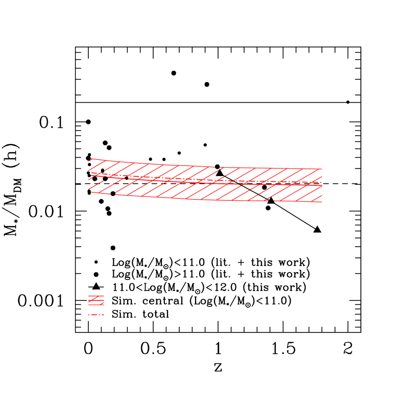
Figure 8: Evolution of the stellar mass fraction for massive galaxies with redshift. The values from our measurements and the literature, as shown in Figure 5, are represented by the dots (small for $M_{*}<10^{11}$$M_{\odot}\,$and enlarged for $M_{*}>10^{11}$$M_{\odot}\,$). The triangle symbols connected by a continuous line represent the measurements made in this study for galaxies with stellar masses $10^{11}$$M_{\odot}\,$$<M_{*}<10^{12}$$M_{\odot}\,$. The red solid line represents the predictions from the De Lucia & Blaizot (2007) model for the central galaxies at $0<z<0.7$ with stellar masses of $M_{*}<10^{11}$$M_{\odot}\,$. The shaded red region is the rms scatter of the observed stellar mass fractions for the central galaxies at $0<z<0.7$. The red dash-dot line shows the prediction from the model for the total stellar mass fraction. The horizontal lines represent the baryonic mass fraction, and the local stellar mass fraction, as described in Figure 6.

In order to verify if the stellar mass fraction derived from the SDSS groups, and the predictions from the De Lucia & Blaizot’s model, are in good agreement, we show in Figure 7 the distribution in stellar mass of satellite galaxies selected in DMHs of masses $10^{13.0}$$h^{-1}M_{\odot}\,$$<M_{\rm DM}<10^{13.5}$$h^{-1}M_{\odot}\,$from the SDSS. This figure shows that the satellite galaxies in the SDSS groups reach a plateau before the completeness limit of $M_{*}=10^{10}$$M_{\odot}\,$, while the number of satellites in the simulations keeps rising. Such a flattening at the faint-end is observed in the luminosity function of the Local Group (e.g. Pritchet & van den Bergh, 1999), confirming that simulations fail to reproduce the luminosity/mass function of satellites galaxies in groups. This is part of the well known missing satellite problem in CDM (e.g. Moore et al., 1999). At the completeness limits of the SDSS data there are twice as many satellites per DMH in the simulations than in the observations. Within the most massive part of this distribution it appears that the simulations lack massive satellite galaxies when compared to the observed SDSS groups. This is more likely due to the limited-volume of the simulations, but could also be due to the lack of massive galaxies in the overall mass functions as discussed above. However, the observations contain many uncertainties as well. Estimating the stellar-masses of faint objects is still tricky, and the group membership of satellite galaxies, especially at the faint end, is difficult to ascertain. To solve this issue, a deeper study of groups and clusters is required to estimate, in a better manner, their total stellar and dark-matter masses.

Finally, Figure 8 shows the variation of the stellar-mass fraction with redshift predicted from the simulation compared to the data themselves. This figure shows that no variation of the stellar mass fraction with redshift is predicted by the simulation for galaxies with stellar masses $M_{*}<10^{11}$$M_{\odot}\,$. The N-body simulations present a very tight correlation between the mass of the DMHs and the number of galaxies hosted by each DMH at any epoch, and are in this sense very close to Smooth Particle Hydrodynamic simulations and analytic Halo Occupation models (e.g. Berlind et al., 2003; Zheng et al., 2005; Weinberg et al., 2008). Therefore, the stellar mass fraction in a given range of stellar mass is constant with epoch, and by construction equal to the mean value in the local Universe, explaining their failure to reproduce the observed increase in stellar mass fraction with lower redshift. Moreover, as shown in Figure 8, the effect of the fraction of mass in satellites is negligible here as well. However, because of the limited volume of the simulations, the number of galaxies with $M_{*}>10^{11}$$M_{\odot}\,$does not allow for a direct comparisons with our observations. Simulations over larger volume are required, and observations of the stellar mass ratio of less massive galaxies at $1.0<z<2.0$ would be very useful as well.

6 Summary

We present in this paper an analysis of the clustering properties of a stellar mass selected sample of galaxies over 0.7 deg² taken from the Palomar Observatory Wide-Field Infrared Survey (POWIR). By utilising information from three separate fields, we measure the two-point correlation function, and based on this we derive the spatial correlation length and bias for our sample of galaxies within various stellar mass bins at $M_{*}>10^{10}$$M_{\odot}\,$. Our major results are:

I. We find that the correlation length ($r_{0}$) varies with both redshift and stellar mass. We find that the largest correlation lengths (most clustered systems) are found for galaxies at the highest stellar masses with $10^{11}$$M_{\odot}\,$$<M_{*}<10^{12}$$M_{\odot}\,$at $z\sim 2$. The correlation length for galaxies at all stellar mass selections are found to decrease at lower redshift.

II. We derive the dark matter halo masses for these stellar mass selected systems utilising the correlation lengths and models from Mo & White (2002). Due to a likely contamination between our samples, the correlation lengths and therefore the dark matter halo masses are lower limit estimates. However we take into account this effect in our error budgets. We find that halo masses for our galaxies selected by $M_{*}>10^{10.5}$$M_{\odot}\,$are a factor of 30 to 170 times the stellar masses of each galaxy. This is in very good agreement with other methods for measuring halo masses, including lensing and kinematics.

III. We find a remarkable relation between dark matter halo mass ($M_{\rm DM}$), and the ratio of stellar-to-dark-matter-mass ($M_{*}/M_{\rm DM}$) for the central galaxy in the halo, and find that this relation does not vary much with redshift. This correlation is such that the more massive a dark matter halo mass $M_{\rm DM}$ is, the lower the ratio of stellar-to-halo-mass ($M_{*}/M_{\rm DM}$). We further find that this correlation exists over at least two orders of magnitude from halo masses $M_{\rm DM}=10^{12.0}$ to $10^{14.0}$$h^{-1}M_{\odot}\,$. This is true for all methods of determining halo masses, from lensing, kinematics, and clustering.

IV. Within our massive galaxy sample at $z\sim 1-2$ we find that the ratio of stellar-to-halo-mass increases from high to low redshifts. This correlation implies that at a given stellar mass selection, the average underlying mass of the host halo decreases at lower redshifts. This may imply that the most stellar massive systems at the highest redshifts are hosted by very massive haloes, but at lower redshift they stop forming new stars, and therefore do not increase their stellar mass, while other systems in the lower mass dark matter haloes grow to reach similar stellar mass. This is an example of “Halo downsizing”. The ‘Halo Assembly bias’ implying that clustering depends not only on the mass of the dark matter halo, but also on the assembly history and environment of the galaxy, can also contribute partially to this observed increase in the stellar mass fraction with redshift.

V. We compare our results to the semi-analytic models built using the Millennium simulation. We find that there is roughly a good agreement between models and the data for the central galaxy. The predicted value of the total-stellar-to-total-halo mass ratio decreases only slightly with increasing halo mass, also in rough agreement with our observational results. We use the SDSS group catalogue from Weinmann et al. (2006) to examine whether the missing stellar mass can be accounted for by observed satellite galaxies. We find that, even though the overall agreement is good, the model marginally overpredicts the number of faint galaxies in comparison to the SDSS catalogue. Moreover the Millennium simulation fails to reproduce the “halo downsizing” effect we observe. We argue that this missing mass, in the more massive haloes, is most probably in the form of baryons in a warm/hot phase.

References

- Arnaud & Evrard (1999) Arnaud, M. & Evrard, A. E. 1999, MNRAS, 305, 631
- Arnouts et al. (1999) Arnouts, S., Cristiani, S., Moscardini, L., et al. 1999, MNRAS, 310, 540
- Baldry et al. (2008) Baldry, I. K., Glazebrook, K., & Driver, S. P. 2008, MNRAS, 388, 945
- Balogh et al. (2008) Balogh, M. L., McCarthy, I. G., Bower, R. G., & Eke, V. R. 2008, MNRAS, 385, 1003
- Balogh et al. (2007) Balogh, M. L., Wilman, D., Henderson, R. D. E., et al. 2007, MNRAS, 374, 1169
- Bamford et al. (2006) Bamford, S. P., Aragón-Salamanca, A., & Milvang-Jensen, B. 2006, MNRAS, 366, 308
- Bardeen et al. (1986) Bardeen, J. M., Bond, J. R., Kaiser, N., & Szalay, A. S. 1986, ApJ, 304, 15
- Bell et al. (2007) Bell, E. F., Zheng, X. Z., Papovich, C., et al. 2007, ApJ, 663, 834
- Benítez (2000) Benítez, N. 2000, ApJ, 536, 571
- Berlind et al. (2003) Berlind, A. A., Weinberg, D. H., Benson, A. J., et al. 2003, ApJ, 593, 1
- Bertin & Arnouts (1996) Bertin, E. & Arnouts, S. 1996, A&A, 117, 393
- Böhm & Ziegler (2007) Böhm, A. & Ziegler, B. L. 2007, ApJ, 668, 846
- Böhm et al. (2004) Böhm, A., Ziegler, B. L., Saglia, R. P., et al. 2004, A&A, 420, 97
- Borch et al. (2006) Borch, A., Meisenheimer, K., Bell, E. F., et al. 2006, A&A, 453, 869
- Bouwens et al. (2007) Bouwens, R. J., Illingworth, G. D., Franx, M., & Ford, H. 2007, ApJ, 670, 928
- Bower et al. (2006) Bower, R. G., Benson, A. J., Malbon, R., et al. 2006, MNRAS, 370, 645
- Bruzual & Charlot (2003) Bruzual, G. & Charlot, S. 2003, MNRAS, 344, 1000
- Bundy et al. (2005) Bundy, K., Ellis, R. S., & Conselice, C. J. 2005, ApJ, 625, 621
- Bundy et al. (2006) Bundy, K., Ellis, R. S., Conselice, C. J., et al. 2006, ApJ, 651, 120
- Bundy et al. (2008) Bundy, K., Georgakakis, A., Nandra, K., et al. 2008, ApJ, 681, 931
- Busha et al. (2005) Busha, M. T., Evrard, A. E., Adams, F. C., & Wechsler, R. H. 2005, MNRAS, 363, L11
- Carroll et al. (1992) Carroll, S. M., Press, W. H., & Turner, E. L. 1992, ARA&A, 30, 499
- Cattaneo et al. (2008) Cattaneo, A., Dekel, A., Faber, S. M., & Guiderdoni, B. 2008, MNRAS, 389, 567
- Chabrier (2003) Chabrier, G. 2003, PASP, 115, 763
- Chiu et al. (2007) Chiu, K., Bamford, S. P., & Bunker, A. 2007, MNRAS, 377, 806
- Cirasuolo et al. (2010) Cirasuolo, M., McLure, R. J., Dunlop, J. S., et al. 2010, MNRAS, 401, 1166
- Cirasuolo et al. (2007) —. 2007, MNRAS, 380, 585
- Coil et al. (2006) Coil, A. L., Newman, J. A., Cooper, M. C., et al. 2006, ApJ, 644, 671
- Coil et al. (2004) Coil, A. L., Newman, J. A., Kaiser, N., et al. 2004, ApJ, 617, 765
- Cole et al. (2001) Cole, S., Norberg, P., Baugh, C. M., et al. 2001, MNRAS, 326, 255
- Collister & Lahav (2004) Collister, A. A. & Lahav, O. 2004, PASP, 116, 345
- Conroy et al. (2009) Conroy, C., Gunn, J. E., & White, M. 2009, ApJ, 699, 486
- Conroy & Wechsler (2009) Conroy, C. & Wechsler, R. H. 2009, ApJ, 696, 620
- Conselice et al. (2003) Conselice, C. J., Bershady, M. A., Dickinson, M., & Papovich, C. 2003, AJ, 126, 1183
- Conselice et al. (2005a) Conselice, C. J., Blackburne, J. A., & Papovich, C. 2005a, ApJ, 620, 564
- Conselice et al. (2005b) Conselice, C. J., Bundy, K., Ellis, R. S., et al. 2005b, ApJ, 628, 160
- Conselice et al. (2007) Conselice, C. J., Bundy, K., Trujillo, I., et al. 2007, MNRAS, 381, 962
- Conselice et al. (2008) Conselice, C. J., Bundy, K., U, V., et al. 2008, MNRAS, 383, 1366
- Cowie & Barger (2008) Cowie, L. L. & Barger, A. J. 2008, ApJ, 686, 72
- Cresswell & Percival (2009) Cresswell, J. G. & Percival, W. J. 2009, MNRAS, 392, 682
- Croton et al. (2007a) Croton, D. J., Gao, L., & White, S. D. M. 2007a, MNRAS, 374, 1303
- Croton et al. (2007b) Croton, D. J., Norberg, P., Gaztañaga, E., & Baugh, C. M. 2007b, MNRAS, 379, 1562
- Croton et al. (2006) Croton, D. J., Springel, V., White, S. D. M., et al. 2006, MNRAS, 365, 11
- Davis et al. (2003) Davis, M., Faber, S. M., Newman, J., et al. 2003, in Discoveries and Research Prospects from 6- to 10-Meter-Class Telescopes II. Edited by Guhathakurta, Puragra. Proceedings of the SPIE, Volume 4834, pp. 161-172 (2003)., 161–172
- Davis et al. (2007) Davis, M., Guhathakurta, P., Konidaris, N. P., et al. 2007, ApJ, 660, L1
- De Lucia & Blaizot (2007) De Lucia, G. & Blaizot, J. 2007, MNRAS, 375, 2
- De Lucia et al. (2006) De Lucia, G., Springel, V., White, S. D. M., Croton, D., & Kauffmann, G. 2006, MNRAS, 366, 499
- Drory & Alvarez (2008) Drory, N. & Alvarez, M. 2008, ApJ, 680, 41
- Drory et al. (2003) Drory, N., Bender, R., Feulner, G., et al. 2003, ApJ, 595, 698
- Drory et al. (2005) Drory, N., Salvato, M., Gabasch, A., et al. 2005, ApJ, 619, L131
- Eke et al. (2004) Eke, V. R., Frenk, C. S., Baugh, C. M., et al. 2004, MNRAS, 355, 769
- Faber et al. (2003) Faber, S. M., Phillips, A. C., Kibrick, R. I., et al. 2003, in Presented at the Society of Photo-Optical Instrumentation Engineers (SPIE) Conference, Vol. 4841, Society of Photo-Optical Instrumentation Engineers (SPIE) Conference Series, ed. M. Iye & A. F. M. Moorwood, 1657–1669
- Fernández Lorenzo et al. (2009) Fernández Lorenzo, M., Cepa, J., Bongiovanni, A., et al. 2009, A&A, 496, 389
- Fontana et al. (2006) Fontana, A., Salimbeni, S., Grazian, A., et al. 2006, A&A, 459, 745
- Förster Schreiber et al. (2006) Förster Schreiber, N. M., Genzel, R., Lehnert, M. D., et al. 2006, ApJ, 645, 1062
- Foucaud et al. (2007) Foucaud, S., Almaini, O., Smail, I., et al. 2007, MNRAS, 376, L20
- Gao et al. (2005) Gao, L., Springel, V., & White, S. D. M. 2005, MNRAS, 363, L66
- Gao & White (2007) Gao, L. & White, S. D. M. 2007, MNRAS, 377, L5
- Gonzalez et al. (2007) Gonzalez, A. H., Zaritsky, D., & Zabludoff, A. I. 2007, ApJ, 666, 147
- Groth & Peebles (1977) Groth, E. J. & Peebles, P. J. E. 1977, ApJ, 217, 385
- Guzzo et al. (1997) Guzzo, L., Strauss, M. A., Fisher, K. B., Giovanelli, R., & Haynes, M. P. 1997, ApJ, 489, 37+
- Hartley et al. (2008) Hartley, W. G., Lane, K. P., Almaini, O., et al. 2008, MNRAS, 391, 1301
- Hoekstra et al. (2001) Hoekstra, H., Franx, M., Kuijken, K., et al. 2001, ApJ, 548, L5
- Ilbert et al. (2005) Ilbert, O., Tresse, L., Zucca, E., et al. 2005, A&A, 439, 863
- Kassin et al. (2007) Kassin, S. A., Weiner, B. J., Faber, S. M., et al. 2007, ApJ, 660, L35
- Kauffmann & Charlot (1998) Kauffmann, G. & Charlot, S. 1998, MNRAS, 297, L23
- Kauffmann et al. (2003) Kauffmann, G., Heckman, T. M., White, S. D. M., et al. 2003, MNRAS, 341, 33
- Kitzbichler & White (2007) Kitzbichler, M. G. & White, S. D. M. 2007, MNRAS, 376, 2
- Komatsu et al. (2009) Komatsu, E., Dunkley, J., Nolta, M. R., et al. 2009, ApJS, 180, 330
- Kroupa (2001) Kroupa, P. 2001, MNRAS, 322, 231
- Landy & Szalay (1993) Landy, S. D. & Szalay, A. S. 1993, ApJ, 412, 64
- Le Fèvre et al. (2005) Le Fèvre, O., Guzzo, L., Meneux, B., et al. 2005, A&A, 439, 877
- Li et al. (2006) Li, C., Kauffmann, G., Jing, Y. P., et al. 2006, MNRAS, 368, 21
- Lin & Mohr (2004) Lin, Y.-T. & Mohr, J. J. 2004, ApJ, 617, 879
- Magliocchetti et al. (2000) Magliocchetti, M., Bagla, J. S., Maddox, S. J., & Lahav, O. 2000, MNRAS, 314, 546
- Magliocchetti et al. (2008) Magliocchetti, M., Cirasuolo, M., McLure, R. J., et al. 2008, MNRAS, 383, 1131
- Magliocchetti & Maddox (1999) Magliocchetti, M. & Maddox, S. J. 1999, MNRAS, 306, 988
- Mandelbaum et al. (2006) Mandelbaum, R., Seljak, U., Kauffmann, G., Hirata, C. M., & Brinkmann, J. 2006, MNRAS, 368, 715
- Marchesini et al. (2009) Marchesini, D., van Dokkum, P. G., Förster Schreiber, N. M., et al. 2009, ApJ, 701, 1765
- McCracken et al. (2008) McCracken, H. J., Ilbert, O., Mellier, Y., et al. 2008, A&A, 479, 321
- McLure et al. (2009) McLure, R. J., Cirasuolo, M., Dunlop, J. S., Foucaud, S., & Almaini, O. 2009, MNRAS, 395, 2196
- Meneux et al. (2008) Meneux, B., Guzzo, L., Garilli, B., et al. 2008, A&A, 478, 299
- Mo & White (2002) Mo, H. J. & White, S. D. M. 2002, MNRAS, 336, 112
- Moore et al. (1999) Moore, B., Ghigna, S., Governato, F., et al. 1999, ApJ, 524, L19
- More et al. (2009) More, S., van den Bosch, F. C., & Cacciato, M. 2009, MNRAS, 392, 917
- Neistein et al. (2006) Neistein, E., van den Bosch, F. C., & Dekel, A. 2006, MNRAS, 372, 933
- Noeske et al. (2007) Noeske, K. G., Faber, S. M., Weiner, B. J., et al. 2007, ApJ, 660, L47
- Norberg et al. (2002) Norberg, P., Baugh, C. M., Hawkins, E., et al. 2002, MNRAS, 332, 827
- Norberg et al. (2001) —. 2001, MNRAS, 328, 64
- Ouchi et al. (2005) Ouchi, M., Hamana, T., Shimasaku, K., et al. 2005, ApJ, 635, L117
- Ouchi et al. (2004) Ouchi, M., Shimasaku, K., Okamura, S., et al. 2004, ApJ, 611, 685
- Peebles (1980) Peebles, J. 1980, The Large-Scale Structure of the Universe (Princeton)
- Pérez-González et al. (2005) Pérez-González, P. G., Rieke, G. H., Egami, E., et al. 2005, ApJ, 630, 82
- Pérez-González et al. (2008) Pérez-González, P. G., Rieke, G. H., Villar, V., et al. 2008, ApJ, 675, 234
- Pollo et al. (2006) Pollo, A., Guzzo, L., Le Fèvre, O., et al. 2006, A&A, 451, 409
- Pozzetti et al. (2007) Pozzetti, L., Bolzonella, M., Lamareille, F., et al. 2007, A&A, 474, 443
- Pritchet & van den Bergh (1999) Pritchet, C. J. & van den Bergh, S. 1999, AJ, 118, 883
- Puech et al. (2008) Puech, M., Flores, H., Hammer, F., et al. 2008, A&A, 484, 173
- Quadri et al. (2007) Quadri, R., van Dokkum, P., Gawiser, E., et al. 2007, ApJ, 654, 138
- Quadri et al. (2008) Quadri, R. F., Williams, R. J., Lee, K., et al. 2008, ApJ, 685, L1
- Reddy et al. (2006) Reddy, N. A., Steidel, C. C., Erb, D. K., Shapley, A. E., & Pettini, M. 2006, ApJ, 653, 1004
- Reddy et al. (2008) Reddy, N. A., Steidel, C. C., Pettini, M., et al. 2008, ApJS, 175, 48
- Roche et al. (1993) Roche, N., Shanks, T., Metcalfe, N., & Fong, R. 1993, MNRAS, 263, 360
- Sheth et al. (2001) Sheth, R. K., Mo, H. J., & Tormen, G. 2001, MNRAS, 323, 1
- Sheth & Tormen (1999) Sheth, R. K. & Tormen, G. 1999, MNRAS, 308, 119
- Skibba et al. (2006) Skibba, R., Sheth, R. K., Connolly, A. J., & Scranton, R. 2006, MNRAS, 369, 68
- Skrutskie et al. (2006) Skrutskie, M. F., Cutri, R. M., Stiening, R., et al. 2006, AJ, 131, 1163
- Sofue & Rubin (2001) Sofue, Y. & Rubin, V. 2001, ARA&A, 39, 137
- Somerville et al. (2004) Somerville, R. S., Lee, K., Ferguson, H. C., et al. 2004, ApJ, 600, L171
- Springel et al. (2005a) Springel, V., Di Matteo, T., & Hernquist, L. 2005a, MNRAS, 361, 776
- Springel et al. (2005b) Springel, V., White, S. D. M., Jenkins, A., et al. 2005b, Nat, 435, 629
- Steidel et al. (2004) Steidel, C. C., Shapley, A. E., Pettini, M., et al. 2004, ApJ, 604, 534
- Swinbank et al. (2006) Swinbank, A. M., Bower, R. G., Smith, G. P., et al. 2006, MNRAS, 368, 1631
- Thomas et al. (2005) Thomas, D., Maraston, C., Bender, R., & Mendes de Oliveira, C. 2005, ApJ, 621, 673
- Tinker et al. (2010) Tinker, J. L., Wechsler, R. H., & Zheng, Z. 2010, ApJ, 709, 67
- Tinker et al. (2005) Tinker, J. L., Weinberg, D. H., Zheng, Z., & Zehavi, I. 2005, ApJ, 631, 41
- Tresse et al. (2007) Tresse, L., Ilbert, O., Zucca, E., et al. 2007, A&A, 472, 403
- Trujillo et al. (2007) Trujillo, I., Conselice, C. J., Bundy, K., et al. 2007, MNRAS, 382, 109
- van den Bosch et al. (2005) van den Bosch, F. C., Yang, X., Mo, H. J., & Norberg, P. 2005, MNRAS, 356, 1233
- van Starkenburg et al. (2008) van Starkenburg, L., van der Werf, P. P., Franx, M., et al. 2008, A&A, 488, 99
- Vikhlinin et al. (2006) Vikhlinin, A., Kravtsov, A., Forman, W., et al. 2006, ApJ, 640, 691
- Warren et al. (2006) Warren, M. S., Abazajian, K., Holz, D. E., & Teodoro, L. 2006, ApJ, 646, 881
- Wechsler et al. (2001) Wechsler, R. H., Somerville, R. S., Bullock, J. S., et al. 2001, ApJ, 554, 85
- Weinberg et al. (2008) Weinberg, D. H., Colombi, S., Davé, R., & Katz, N. 2008, ApJ, 678, 6
- Weiner et al. (2006) Weiner, B. J., Willmer, C. N. A., Faber, S. M., et al. 2006, ApJ, 653, 1049
- Weinmann et al. (2006) Weinmann, S. M., van den Bosch, F. C., Yang, X., & Mo, H. J. 2006, MNRAS, 366, 2
- Whiley et al. (2008) Whiley, I. M., Aragón-Salamanca, A., De Lucia, G., et al. 2008, MNRAS, 387, 1253
- White & Frenk (1991) White, S. D. M. & Frenk, C. S. 1991, ApJ, 379, 52
- Yang et al. (2005) Yang, X., Mo, H. J., van den Bosch, F. C., & Jing, Y. P. 2005, MNRAS, 357, 608
- Yoshida et al. (2008) Yoshida, M., Shimasaku, K., Ouchi, M., et al. 2008, ApJ, 679, 269
- Zehavi et al. (2004) Zehavi, I., Weinberg, D. H., Zheng, Z., et al. 2004, ApJ, 608, 16
- Zehavi et al. (2005) Zehavi, I., Zheng, Z., Weinberg, D. H., et al. 2005, ApJ, 630, 1
- Zheng et al. (2005) Zheng, Z., Berlind, A. A., Weinberg, D. H., et al. 2005, ApJ, 633, 791
- Zheng et al. (2007) Zheng, Z., Coil, A. L., & Zehavi, I. 2007, ApJ, 667, 760