Neutral weak currents in nucleon superfluid Fermi liquids:
Larkin-Migdal and Leggett approaches

Abstract

Neutrino emission in processes of breaking and formation of nucleon Cooper pairs is calculated in the framework of the Larkin-Migdal and the Leggett approaches to the description of superfluid Fermi liquids at finite temperatures. We explain peculiarities of both approaches and explicitly demonstrate that they lead to the same expression for the emissivity in pair breaking and formation processes.

I Introduction

One of important mechanisms for cooling of superfluid neutron star interiors is nucleon Cooper pair breaking and formation (PBF) with a radiation of neutrino-antineutrino pairs, $"N"\to"N"+\nu+\bar{\nu}$ (see FRS76 ; VS87 ; SV87 ; MSTV90 ; SVSWW97 ; Minimal ; KHY ; YKL99 ; YLS99 ; V01 ; BGV04 ; GV05 ; PGW ; Sedr07 ; KR ; LP ; SMS ; KV08 ; L08 ; SR09 ; LeinsonWrong and references therein). Neutrinos are produced in weak interactions in which the lepton current $l_{\mu}=\bar{\nu}(1-\gamma_{5})\nu$ is coupled to the vector ($V_{\mu}=g_{V}\,\bar{\Psi}\,\gamma^{\mu}\,\Psi$) and the axial-vector ($A_{\mu}=g_{A}\,\bar{\Psi}\,\gamma^{\mu}\gamma_{5}\,\Psi$) nucleon currents; $\mathcal{L}=-\frac{G}{2\,\sqrt{2}}\,(V^{\mu}-A^{\mu})\,l_{\mu}$, where $G\approx 1.2\times 10^{-5}$ GeV^-2 is the weak interaction coupling, $g_{V}=-1$ and $g_{A}=1.26$. For the nuclear vector current holds $\partial_{\mu}V^{\mu}=0$ that corresponds to the conservation of the baryon charge. Early works FRS76 ; VS87 ; SV87 ; MSTV90 ; SVSWW97 ; Minimal ; KHY ; YKL99 ; YLS99 ; V01 ; BGV04 ; GV05 ; PGW ; Sedr07 did not care about the vector-current conservation. The latter is fulfilled only if in-medium renormalization of the vector current is performed together with a corresponding renormalization of Green’s functions. This problem was tackled in Refs. KR ; LP ; SMS ; KV08 ; L08 ; SR09 ; PLPS . Reference LP indicated that the emissivity of the $1S_{0}$ PBF processes on the vector current should be dramatically suppressed ($\propto v_{\rm F}^{4}$, where $v_{\rm F}$ is the Fermi velocity of non-relativistic nucleons) provided the vector current conservation is fulfilled. Reference LP used expressions derived within the standard BCS formalism of the superconductivity theory Nambu ; Schriffer for low excitation energies $\omega,|\vec{q}|\ll\Delta$, where $\Delta$ is the nucleon pairing gap and $\omega$ is the net $\nu\bar{\nu}$ energy, whereas the PBF reaction kinematics permits only $\omega>2\Delta$, $|\vec{q}|<\omega$. The correlation effects in the particle-hole channel were neglected and processes induced by the axial-vector current were disregarded.

The consistent calculation of the PBF emissivity induced by the vector and axial-vector currents was performed in Ref. KV08 within the Larkin-Migdal-Leggett Fermi liquid approach. The latter takes properly into account of the correlation effects in both particle-particle and particle-hole channels. It was demonstrated that the neutrino emissivity is actually controlled by the axial-vector current and is suppressed only by the factor $\propto v_{\rm F}^{2}$, rather than $\propto v_{\rm F}^{4}$ as was stated in Ref. LP . This result was supported in the subsequent work L08 , which however continued to work out the vector current contribution neglecting the correlation effects in the particle-hole channel.

The convenient Nambu-Gorkov formalism developed for the description of metallic superconductors, cf. Refs. Nambu ; Schriffer , does not distinguish interactions in particle-particle and particle-hole channels. These interactions can be, however, essentially different in strongly interacting matter, like in nuclear matter and in liquid He³. The adequate methods for Fermi liquids with pairing were developed for zero temperature by Larkin and Migdal in Ref. LM63 (see also M67 ) and for a finite temperature by Leggett in Ref. Leg65a ; L66 . The problem of calculation of a response function of a Fermi system to an external interaction becomes tractable at cost of introduction of a set of Landau-Migdal parameters for quasiparticle interactions. Parameters can be either evaluated microscopically or extracted from analysis of experimental data, see M67 . The technical difference of the mentioned approaches is that Larkin and Migdal worked out equations for full in-medium vertices, whereas Leggett calculated directly a response function. The former approach was aimed at the study of transitions in nuclei, and the latter on the analyzes of collective modes in superfluid Fermi liquid. The principal equivalence of both approaches was emphasized by Leggett in Ref. Leg65a ; L66 .

In Ref. KV08 we used the Larkin-Migdal approach. More specifically, we solved the Larkin-Migdal equations for the vertices induced by the weak vector and axial-vector currents and calculated the current-current correlation function $\chi_{a}$, $a=\{V,A\}$, and the PBF emissivity. The explicit expression for $\chi_{a}$ was obtained at $T=0$. It is sufficient to calculate emissivity of the process for $T\ll 2\Delta$ since small exponential factor $e^{-2\Delta/T}$ comes already from the phase space volume and the temperature correction to $\chi_{a}(T=0)$ is small in this limit. Despite Larkin-Migdal equations were derived in their original paper for $T=0$, actually the results can be generalized for arbitrary $T$. In Ref. KV08 we sketched which expressions should be modified at finite temperatures.

Recent paper LeinsonWrong tried to adopt the Leggett formalism to calculate the PBF emissivity for the $1S_{0}$ neutron pairing and came to different results compared to those derived in Ref. KV08 , even in case $T\ll\Delta$. One of the points of Ref. LeinsonWrong was to find the PBF emissivity for arbitrary $T\neq 0$. In view of the explicit claim by Leggett in Ref. L66 on the equivalence of his approach to that of Larkin and Migdal, this difference looks worrisome and requires a clarification.

The aim of this paper is to reveal the correspondence between the Larkin-Migdal and Leggett approaches and to generalize the results of Ref. KV08 to arbitrary temperatures. We argue also that the results of the work LeinsonWrong are based on misinterpretation and wrong solution of the Leggett equations.

The paper is organized as follows. In Section II we introduce the Fermi liquid approach to the problem of the neutrino emissivity from nucleon matter. We focus on the emissivity via the PBF reactions. The main expressions are presented in the diagrammatic form valid at arbitrary temperatures. Then in Section III we demonstrate how the Larkin-Migdal equations and the Leggett equations follow from the same set of diagrams. In Section IV we solve the Larkin-Migdal equations for the vertices induced by the vector and axial-vector currents and, then, present expressions for the PBF emissivity recovering the results of Ref. KV08 formulated now for arbitrary temperatures. In Section V we demonstrate how the same results can be obtained within the Leggett formalism. In Section VI we discuss the flaws in Ref. LeinsonWrong . We conclude with Section VII.

II General expressions for neutrino emissivity and current-current correlators

In this section we recall the main expressions for the neutrino emissivity obtained in Ref. KV08 , writing them in the form valid at arbitrary temperatures. To be specific we consider a neutron system with the s-wave pairing. The neutrino emissivity

$$\varepsilon_{\nu\bar{\nu}}=\frac{G^{2}}{4}\intop\prod_{i=1}^{2}\frac{d^{3}{q}_{i}}{(2\pi)^{3}\,2\,\omega_{i}}\frac{(\omega_{1}+\omega_{2})\,\Im\sum\chi(q_{1}+q_{2})}{e^{(\omega_{1}+\omega_{2})/T}-1}$$ (1)

is expressed through the imaginary part of the Fourier-transform of the current-current correlator $\chi(q)=\chi_{V}(q)+\chi_{A}(q)=\int{\rm d}^{4}xe^{-i\,(q\cdot x)}\langle N|\big{(}V^{\mu}(x)\,V^{\nu}(0)+A^{\mu}(x)\,A^{\nu}(0)\big{)}\,l_{\mu}(x)l_{\nu}^{\dagger}(0)|N\rangle$ , where $q=(\omega_{1}+\omega_{2},\vec{q}_{1}+\vec{q}_{2})$. The averaging is done over the vector of state, $|N\rangle$, of the fermion system with pairing at thermal equilibrium. The summation runs over the lepton spins.

We use non-relativistic limit for nucleons since the nucleon Fermi energy $\epsilon_{{\rm F}}\ll m$, where $m$ is the nucleon mass. The bare vertices for the nucleon currents as they follow from the expansion of the Lagrangian are $V^{0\mu}\approx\psi^{\dagger}\big{(}{p}^{\prime})\,(1,\,(\vec{p\,}^{\prime}+\vec{p\,})/2\,m\big{)}\,\psi(p)$ and $A^{0\mu}\approx\psi^{\dagger}(p^{\prime})\,\big{(}\vec{\sigma}(\vec{p\,}^{\prime}+\vec{p\,})/2\,m,\,\vec{\sigma}\big{)}\,\psi(p)$ , where $\vec{\sigma}=(\sigma_{1},\sigma_{2},\sigma_{3})$ are the Pauli matrices acting on free nucleon spinors $\psi$, and $\vec{p\,}^{\prime}$ and $\vec{p\,}$ are outgoing and incoming momenta.

In a system with pairing a particle can transit into a hole and a condensate pair and vice versa. The one-particle one-hole irreducible amplitudes of such processes are depicted in Fig. 1.

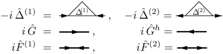
Figure 1: Amplitudes of the transition of a particle into a hole and a condensate pair, $\Delta^{(1)}$ and vice versa, $\Delta^{(2)}$, and normal, $G$, and anomalous, $F$, Green’s functions.

Besides the normal Green’s function $\,\hat{G}$  one introduces anomalous Green’s functions $\hat{F}^{(1)}$ , and $\hat{F}^{(2)}$ , which diagrammatic notations are given in Fig. 1. The Green’s function for the hole is defined as $\hat{G}^{h}(p)=\hat{G}^{\rm T}(-p)$ . Superscript $\rm T$ denotes matrix transposition. The normal and anomalous Green’s functions are related by Gor’kov equations. The normal Green’s function is diagonal in spin space $\hat{G}(p)=G(p)\,\hat{1}$, but the anomalous Green’s functions are equal to $\hat{F}^{(1)}(p)=\hat{F}^{(2)}(p)=\hat{F}(p)=F(p)\,i\sigma_{2}$. We will not discuss here the details of the Fermi liquid renormalization procedure, see Refs. Migdal63 ; LM63 ; Leg65a ; M67 . The latter allows to separate contributions from the pole and regular parts of the Green’s functions in all relevant quantities. We assume that this procedure is properly done and we deal further only with the pole parts of the Green’s functions characterized by the effective mass $m^{*}$ and the residue $a$:

$$G(p)=\frac{a\,(\epsilon+\epsilon_{p})}{\epsilon^{2}-E_{p}^{2}+i0{\rm sgn}\epsilon},\,F(p)=\frac{-a\,\Delta}{\epsilon^{2}-E_{p}^{2}+i0{\rm sgn}\epsilon}\,,$$ (2)

where $E_{p}^{2}=\epsilon_{p}^{2}+\Delta^{2}$ with the pairing gap $\Delta$, and $\epsilon_{p}=p^{2}/(2\,m^{*})-\mu(T)$, $\mu$ is the chemical potential, $\mu(T=0)=\epsilon_{\rm F}=p_{\rm F}^{2}/(2\,m^{*})$. At finite temperature one can use the Matsubara techniques with the replacement $\epsilon\to i\,\epsilon_{n}=i\,\pi(2n+1)$ .

The amplitude in the particle-particle channel is parameterized as

$$\big{[}\widehat{\Gamma}^{\xi}\big{]}^{ac}_{bd}=\Gamma_{0}^{\xi}(\vec{n},\vec{n\,}^{\prime})(i\sigma_{2})^{a}_{b}(i\sigma_{2})^{c}_{d}+\Gamma^{\xi}_{1}(\vec{n},\vec{n\,}^{\prime})(i\sigma_{2}\,\vec{\sigma})^{a}_{b}(\vec{\sigma}\,i\sigma_{2})^{c}_{d},$$

and the interaction in the particle-hole channel is

$$\big{[}\widehat{\Gamma}^{\omega}\big{]}^{ac}_{bd}=\Gamma_{0}^{\omega}(\vec{n},\vec{n\,}^{\prime})\,\delta^{a}_{b}\,\delta^{c}_{d}+\Gamma^{\omega}_{1}(\vec{n},\vec{n\,}^{\prime})\,(\vec{\sigma})^{a}_{b}\,(\vec{\sigma})^{c}_{d}.$$

Here and below $\vec{n}=\vec{p}/|\vec{p\,}|$ and $\vec{n\,}^{\prime}=\vec{p\,}^{\prime}/|\vec{p\,}^{\prime}|$ . Superscript ”$\omega$” indicates that the amplitude is taken for $|\vec{q\,}\vec{v\,}_{{\rm F}}|\ll\omega$ and $\omega\ll\epsilon_{{\rm F}}$, where $\omega$ and $\vec{q}$ are transferred energy and momentum. We use that $\epsilon_{\vec{p}+\vec{q}/2}\approx\epsilon_{p}+\vec{v}\,\vec{q}/2$, where $\vec{v}$ is the nucleon velocity at the Fermi surface, $\vec{v}=v_{\rm F}\,\vec{n}(1+O(T^{2}/\epsilon_{\rm F}^{2}))$. Since in the PBF processes $|\vec{q}\,|\stackrel{{\scriptstyle\scriptstyle<}}{{\phantom{}{}_{\sim}}}\Delta$, $\omega\sim 2\Delta$, the terms neglected are of the order of $O(\Delta^{2}/p_{\rm F}^{2})$. Actually, the denominators of the Green’s functions are $|\omega\pm(\epsilon_{\vec{p}+\vec{q}/2}-\epsilon_{\vec{p}-\vec{q}/2})|\ll\epsilon_{{\rm F}}$. Moreover, the terms $\propto\vec{v}\,\vec{q}$ may vanish under the angular integrations. Taking this into account we estimate that the neglected terms are at most of the order of $\Delta/\epsilon_{\rm F}\ll 1$ compared to the retained terms. Such corrections are usually omitted in most calculations within the Fermi liquid theory for superfluids.

The empirical information is usually expressed in terms of dimensionless parameters

$$\Gamma_{0}^{\omega,\xi}(\vec{n},\vec{n\,}^{\prime})=\frac{f^{\omega,\xi}(\vec{n},\vec{n\,}^{\prime})}{a^{2}\rho(n_{0})}\,,\,\,\Gamma_{1}^{\omega,\xi}(\vec{n},\vec{n\,}^{\prime})=\frac{g^{\omega,\xi}(\vec{n},\vec{n\,}^{\prime})}{a^{2}\rho(n_{0})}\,,$$ (3)

where $\rho=\frac{m^{*}\,p_{{{\rm F}}}}{\pi^{2}}$ is the density of states at the Fermi surface.

The pairing gap is determined by the $\Gamma_{0}^{\xi}$ term in the particle-particle interaction, and the gap equation reads

$$\Delta(\vec{n})=-\langle\Gamma_{0}^{\xi}(\vec{n},\vec{n}^{\prime})\,A_{0}(\Delta(\vec{n\,}^{\prime}))\,\Delta(\vec{n\,}^{\prime})\rangle_{\vec{n}^{\prime}}\,,$$ (4)

$$A_{0}(\Delta)=\int{\rm d}\Phi_{T}G_{0}(p)\,G^{h}(p)\,\theta(\xi-\epsilon_{p}),$$ (5)

where $G_{0}(p)=1/(\epsilon-\epsilon_{p}+i0{\rm sgn}\epsilon)$ is the Green’s function for the Fermi system without pairing ($\Delta=0$), and $\xi\sim\mu$ is the cutting parameter. Usually the gap is determined with $\xi=\mu$. We use the following notations for the angular integration

$$\langle\dots\rangle_{\vec{n}} = \int\frac{{\rm d}\Omega_{\vec{n}}}{4\pi}\,(\dots)\,,$$ (6)

and for the integration

$$\int{\rm d}\Phi_{T}\,f(\epsilon,\epsilon_{p})=\left\{\begin{array}[]{cc}\displaystyle\rho\,\int_{-\infty}^{+\infty}\frac{{\rm d}\epsilon}{2\pi i}\int_{-\infty}^{+\infty}{\rm d}\epsilon_{p}f(\epsilon,\epsilon_{p})&\mbox{for}~{}T=0\\ \displaystyle\rho\,T\sum_{n=-\infty}^{\infty}\int_{-\infty}^{+\infty}{\rm d}\epsilon_{p}f(i\epsilon_{n},\epsilon_{p})&\mbox{for}~{}T\neq 0\end{array}\right.\,.$$ (9)

Note that the same value $A_{0}$ can be introduced as $A_{0}=\int{\rm d}\Phi_{T}\,(G(p)\,G^{h}(p)+F(p)\,F(p))\,\theta(\xi-\epsilon_{p})$, cf. Ref. L66 .

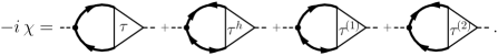
Figure 2: Diagrams contributing to the susceptibility $\chi$ in (1).

The diagrammatic representation for the current-current correlator entering (1) is shown in Fig. 2. The dash line relates to the $Z$-boson coupled to the neutral lepton currents. In terms of the Green’s functions and the quasiparticle interactions we write it as

$$\chi_{a}(\omega,\vec{q}\,)=\frac{1}{2}{\rm Tr}\Big{\langle}\int d\Phi_{T}\hat{\tau}_{a}^{\omega}\,\Big{\{}\hat{G}_{+}\,\hat{\tau}_{a}\,\hat{G}_{-}+\hat{F}_{+}\,\hat{\tau}_{a}^{h}\,\hat{F}_{-}+\hat{G}_{+}\,\hat{\tau}_{a}^{(1)}\hat{F}_{-}+\hat{F}_{+}\,\hat{\tau}_{a}^{(2)}\hat{G}_{-}\Big{\}}\Big{\rangle}_{\vec{n}}\,,$$ (10)

$a=V$ for the vector current and $a=A$ for the axial-vector currents. The trace is taken in the nucleon spin space. Doing calculations in Matsubara technique, we use notations: $G_{+}=G(p_{0}+\omega,\vec{p}+\vec{q}/2)$ and $G_{-}=G(p_{0},\vec{p}-\vec{q}/2)$, and similarly for $F_{\pm}$ functions. For continues frequencies we use the symmetrical 4-vector notations, i.e. $G_{\pm}=G(p\pm q/2)$ and, analogously, $F_{\pm}=F(p\pm q/2)$. The left vertices in Fig. 2 are the bare vertices generated by the weak currents

$$\hat{\tau}^{\omega}_{V}(\vec{n},q) = g_{V}\,\big{(}\tau^{\omega}_{V,0}\,l_{0}-\vec{\tau}^{\omega}_{V,1}\,\vec{l}\,\,\big{)}\hat{1}\,,\quad\tau^{\omega}_{V,0}=\frac{e_{V}}{a}\,\,,\quad\vec{\tau\,}^{\omega}_{V,1}=\frac{e_{V}}{a}\,\vec{v},$$ (11a)

$$\hat{\tau}^{\omega}_{A}(\vec{n},q) = -g_{A}\,\big{(}\vec{\tau\,}^{\omega}_{A,1}\,\vec{\sigma}\,l_{0}-\tau^{\omega}_{A,0}\,\vec{\sigma}\vec{l}\,\,\big{)}\,,\quad\tau^{\omega}_{A,0}=\frac{e_{A}}{a}\,,\quad\vec{\tau\,}^{\omega}_{A,1}=\frac{e_{A}}{a}\,\vec{v}\,,$$ (11b)

$e_{V}$ and $e_{A}$ are effective charges of the vector and axial-vector currents, cf. KV08 . The corresponding vertices for holes are defined as

$$\hat{\tau}^{\omega,h}_{V}(\vec{n},q) = [\hat{\tau}^{\omega}_{V}(-\vec{n},q)]^{\rm T}=g_{V}\,\big{(}\tau^{\omega}_{V,0}\,l_{0}+\vec{\tau\,}^{\omega}_{V,1}\,\vec{l}\,\,\big{)}\hat{1},$$ (12a)

$$\hat{\tau}^{\omega,h}_{A}(\vec{n},q) = [\hat{\tau}^{\omega}_{A}(-\vec{n},q)]^{\rm T}=-g_{A}\,\big{(}-\vec{\tau\,}^{\omega}_{A,1}\,\vec{\sigma\,}^{\rm T}\,l_{0}-\tau^{\omega}_{A,0}\,\vec{\sigma\,}^{\rm T}\vec{l}\,\,\big{)}\,.$$ (12b)

We used here explicitly that $\tau^{\omega}_{a,0}(-p,q)=\tau^{\omega}_{a,0}(p,q)$ and $\vec{\tau\,}^{\omega}_{a,1}(-p,q)=-\vec{\tau\,}^{\omega}_{a,1}(p,q)$.

The right vertices in Fig. (2) are the full in-medium-dressed vertices, which are functions of the out-going frequency $\omega$ and momentum $\vec{q}$, and the nucleon velocity $\vec{v}\simeq v_{\rm F}\,\vec{n}$, $\vec{n}=\vec{p}/p$ . In absence of external magnetic field the spin structure of the full vertex is the same as the spin structure of the bare vertex. Therefore, we write

$$\hat{\tau}_{V} = g_{V}\,\big{(}\tau_{V,0}\,l_{0}-\vec{\tau}_{V,1}\,\vec{l\,}\big{)}\,\hat{1}\,,\quad\hat{\tau}^{h}_{V}=g_{V}\,\big{(}\tau_{V,0}^{h}\,l_{0}-\vec{\tau\,}_{V,1}^{h}\,\vec{l}\,\,\big{)}\,\hat{1}\,,$$ (13a)

$$\hat{\tau}_{V}^{(1)} = (\hat{\tau}_{V}^{(2)})^{\dagger}=-g_{V}\,\big{(}\widetilde{\tau}_{V,0}\,l_{0}-\vec{\widetilde{\tau}}_{V,1}\,\vec{l}\,\,\big{)}\,i\,\sigma_{2}\,,$$ (13b)

$$\hat{\tau}_{A} = -g_{A}\,\big{(}\vec{\tau}_{A,1}\vec{\sigma}\,l_{0}-\tau_{A,0}\,\vec{\sigma}\vec{l}\,\,\big{)}\,,\quad\hat{\tau}^{h}_{A}=-g_{A}\,\big{(}\vec{\tau\,}_{A,1}^{h}\vec{\sigma}^{\rm T}\,l_{0}-\tau_{A,0}^{h}\,\vec{\sigma\,}^{\rm T}\vec{l}\,\,\big{)}\,,$$ (13c)

$$\hat{\tau}^{(1)}_{A} = (\hat{\tau}^{(2)}_{A})^{\dagger}=+g_{A}\,\big{(}\vec{\widetilde{\tau}}_{A,1}\,\vec{\sigma}\,l_{0}-\widetilde{\tau}_{A,0}\,\vec{\sigma}\,\vec{l}\,\,\big{)}\,i\,\sigma_{2}\,.$$ (13d)

We anticipate here the relation between the vertices $\hat{\tau}^{(1)}$ and $\hat{\tau}^{(2)}$, which will be proven later. The full vertices are determined by the diagramatic equations depicted in Fig. 3.

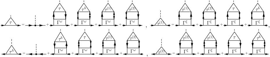
Figure 3: Graphical representation of dressed vertices in Fig. 2.

These graphical equations were first introduced by Larkin and Migdal LM63 . The blocks in Fig. 3 correspond to the two-particle irreducible interaction in the particle-particle channel, $\Gamma^{\xi}$, and the particle-hole irreducible interaction in the particle-hole channel, $\Gamma^{\omega}$. We emphasize that only chains of bubble diagrams are summed up in this particular formulation. Thus, the imaginary part of $\chi$ accounts only for one-nucleon processes. To include two-nucleon processes within a quasi-particle approximation, one should add diagrams with self-energy insertions to the Green’s functions and iterate the Landau-Migdal amplitudes $\Gamma^{\omega,\xi}$ in Fig. 3 in the horizontal channel KV95 .

Working out the spin structure in (10) we obtain

$$\chi_{V}(q)=g_{V}^{2}\,\big{\langle}\big{(}\tau_{V,0}^{\omega}\,l_{0}-\vec{\tau\,}^{\omega}_{V,1}\,\vec{l}\,\big{)}\,\big{(}l_{0}\,\chi_{V,0}(\vec{n},q)-\vec{\chi}_{V,1}(\vec{n},q)\,\vec{l}\,\,\big{)}\big{\rangle}_{\vec{n}},$$ (14a)

$$\chi_{A}(q)=g_{A}^{2}\,\big{\langle}\big{(}\vec{\tau\,}^{\omega}_{A,1}\,l_{0}-\tau_{A,0}^{\omega}\,\vec{l}\,\big{)}\,\big{(}l_{0}\,\vec{\chi}_{A,1}(\vec{n},q)-\chi_{A,0}(\vec{n},q)\vec{l}\,\,\big{)}\big{\rangle}_{\vec{n}},$$ (14b)

where we introduced new scalar and vector response functions

$$\chi_{a,0}(\vec{n},q)=\intop{\rm d}\Phi_{T}\big{(}G_{+}\,G_{-}\,\tau_{a,0}-F_{+}\,F_{-}\,\tau^{h}_{a,0}+(G_{+}\,F_{-}-F_{+}\,G_{-})\,\widetilde{\tau}_{a,0}\big{)}\,,$$ (15a)

$$\vec{\chi}_{a,1}(\vec{n},q)=\intop{\rm d}\Phi_{T}\big{(}G_{+}\,G_{-}\,\vec{\tau}_{a,1}+F_{+}\,F_{-}\,\vec{\tau\,}^{h}_{a,1}+(G_{+}\,F_{-}-F_{+}\,G_{-})\,\widetilde{\vec{\tau}}_{a,0}\big{)}\,.$$ (15b)

It is instructive to express susceptibilities (14a) and (14b) in terms of the polarization tensors

$$\chi_{a}(q)=l_{\mu}\,\Pi_{a}^{\mu\nu}(q)\,l_{\nu}\,.$$

The polarization tensors can be written through the auxiliary bare and dressed currents, $\hat{J}_{a,\mu}^{\omega}(\vec{n},q)$ and $\hat{J}_{a,\mu}(\vec{n},q)$, respectively,

$$\Pi_{a}^{\mu\nu}(q)=\frac{1}{2}\langle{\rm Tr}\{\hat{J}_{a}^{\omega,\mu}(\vec{n},q)\,\hat{J}_{a}^{\nu}(\vec{n},q)\}\rangle_{\vec{n}}\,,$$ (16)

where the vector currents are

$$\hat{J}_{V}^{\omega,\mu}(\vec{n},q)=\big{(}\tau_{V,0}^{\omega},\vec{\tau\,}^{\omega}_{V,1}\big{)}\,\hat{1}\,,\quad\hat{J}_{V}^{\mu}(\vec{n},q)=\big{(}\chi_{V,0},\vec{\chi}_{V,1}\big{)}\,\hat{1}\,,$$ (17)

and the axial-vector currents are

$$\hat{J}_{A}^{\omega,\mu}(\vec{n},q)=\big{(}\vec{\sigma\,}\vec{\tau\,}^{\omega}_{A,1},\vec{\sigma\,}\tau_{A,0}^{\omega}\big{)}\,,\quad\hat{J}_{A}^{\mu}(\vec{n},q)=\big{(}\vec{\sigma\,}\vec{\chi\,}_{A,1},\vec{\sigma\,}\chi_{A,0}\big{)}\,.$$ (18)

Thus, the polarization tensors can be cast as

$$\Pi_{V}^{\mu\nu} = \left(\begin{array}[]{cc}\Pi_{V}^{00},&\Pi_{V}^{0j}\\ \Pi_{V}^{i0},&\Pi_{V}^{ij}\end{array}\right)=\left(\begin{array}[]{cc}\langle\tau^{\omega}_{V,0}\,\chi_{V,0}\rangle_{\vec{n}},&\langle\tau^{\omega}_{V,0}\,(\vec{\chi\,}_{V,1})_{j}\rangle_{\vec{n}}\\ \langle(\vec{\tau\,}^{\omega}_{V,1})_{i}\,\chi_{V,0}\rangle_{\vec{n}},&\langle(\vec{\tau\,}^{\omega}_{V,1})_{i}\,(\vec{\chi}_{V,1})_{j}\rangle_{\vec{n}}\end{array}\right)\,,$$ (23)

$$\Pi_{A}^{\mu\nu} = \left(\begin{array}[]{cc}\Pi_{A}^{00},&\Pi_{A}^{0j}\\ \Pi_{A}^{i0},&\Pi_{A}^{ij}\\ \end{array}\right)=\left(\begin{array}[]{cl}\langle\vec{\tau\,}^{\omega}_{A,1}\vec{\chi}_{A,1}\rangle_{\vec{n}},&\langle\tau^{\omega}_{A,0}\,(\vec{\chi\,\,}_{A,1})_{j}\rangle_{\vec{n}}\\ \langle(\vec{\tau\,}^{\omega}_{A,1})_{i}\,\chi_{A,0}\rangle_{\vec{n}},&\langle\tau^{\omega}_{A,0}\,\chi_{A,0}\rangle_{\vec{n}}\,\delta^{ij}\\ \end{array}\right)\,.$$ (28)

The integration over the lepton phase space can be performed analytically, cf. KV08 , and the neutrino emissivity is then cast in terms of the polarization tensor as

$$\varepsilon_{\nu\nu} = \varepsilon_{\nu\nu,V}+\varepsilon_{\nu\nu,A}\,,$$

$$\varepsilon_{\nu\nu,a} = \frac{G^{2}}{48\,\pi^{4}}\,\int^{\infty}_{0}\!\!{\rm d}\omega\int_{0}^{\omega}\!\!{\rm d}|\vec{q\,}|\frac{\omega\,\vec{q\,}^{2}}{e^{\omega/T}-1}\,K_{a}(q)\,,$$ (29)

$$K_{a}(q) = \big{(}q_{\mu}\,q_{\nu}-g_{\mu\nu}\,q^{2}\big{)}\,\Im\Pi_{a}^{\mu\nu}(q)\,.$$ (30)

The polarization tensor for the conserving vector current must be transverse $\Pi_{V}^{\mu\nu}q_{\nu}=q_{\mu}\,\Pi_{V}^{\mu\nu}=0$. This property will be explicitly proven below in Section IV and in Appendix B. Taking it into account and using (23,28) we find

$$K_{V}(q) = \frac{e_{V}\,g_{V}^{2}}{a}(\vec{q\,}^{2}-\omega^{2})\,\Im\langle\chi_{V,0}(\vec{n},q)-\vec{v}\,\vec{\chi}_{V,1}(\vec{n},q)\rangle_{\vec{n}}\,,$$ (31)

$$K_{A}(q) = \frac{e_{A}\,g_{A}^{2}}{a}\Im\big{[}\vec{q\,}^{2}\langle\vec{v}\,\vec{\chi}_{A,1}(\vec{n},q)\rangle_{\vec{n}}+(3\,\omega^{2}-2\,\vec{q\,}^{2})\,\langle\chi_{A,0}(\vec{n},q)\rangle_{\vec{n}}$$ (32)

$$- \omega\langle\vec{q}\,\vec{\chi}_{A,1}(\vec{n},q)\rangle_{\vec{n}}-\omega\,\langle(\vec{q}\,\vec{v}\,)\,\chi_{A,0}(\vec{n},q)\rangle_{\vec{n}}\big{]}\,.$$

Finally, once the full in-medium vertices (13a,13b,13c,13d) are known, expressions (29,31,32) together with (15a,15b) solve the problem of neutrino emission from superfluid neutron matter via the PBF reactions.

In the rest of the paper we demonstrate two methods for the calculation of the full vertices.

III Correspondence between Larkin-Migdal and Leggett formalisms

The coupling of an external field to the non-relativistic fermion is described by the $2\times 2$ matrix acting in the fermion spin space. Any rank-2 matrix can be decomposed into a unity matrix and Pauli matrices $\vec{\sigma}$. Thus, we have

$$\hat{\tau}(\vec{n},q) = t_{0}(\vec{n},q)\,\hat{1}+\vec{\sigma}\,\vec{t}_{1}(\vec{n},q)\,,$$

$$\hat{\tau}^{(1)}(\vec{n},q) = \big{(}t_{0}^{(1)}(\vec{n},q)\,\hat{1}+\vec{\sigma}\,\vec{t}_{1}^{\,\,(1)}(\vec{n},q)\big{)}\,i\sigma_{2},$$

$$\hat{\tau}^{(2)}(\vec{n},q) = i\sigma_{2}\,\big{(}t_{0}^{(2)}(\vec{n},q)\,\hat{1}+\vec{\sigma}\,\vec{t}_{1}^{\,\,(2)}(\vec{n},q)\big{)}\,.$$ (33)

The hole-vertex is decomposed as

$$\hat{\tau}^{h}(\vec{n},q)=t_{0}^{h}(\vec{n},q)\,\hat{1}+\vec{\sigma}^{\,\rm T}\vec{t}_{1}^{\,h}(\vec{n},q)=t_{0}(-\vec{n},q)\,\hat{1}+\vec{\sigma}^{\,\rm T}\vec{t}(-\vec{n},q).$$ (34)

The spin structures of the weak coupling vertices (11) and (13), we primarily deal with, demonstrate that the vector current contributes only to the vertices with subscript 0 and the axial-vector current couples only to the vertices with subscript 1. E.g., for the vector current

$$t_{0}^{\omega} = g_{V}\,\big{(}\tau_{V,0}^{\omega}\,l_{0}-\vec{\tau\,}_{V,1}^{\omega}\,\vec{l\,}\big{)}\,,$$

$$t_{0} = g_{V}\,\big{(}\tau_{V,0}\,l_{0}-\vec{\tau\,}_{V,1}\,\vec{l\,}\big{)}\,,$$

$$\vec{t\,}_{1}^{\omega} = \vec{t}_{1}=0\,,$$ (35)

and for the axial-vector current

$$t_{0}^{\omega} = t_{0}=0\,,$$

$$\vec{t\,}_{1}^{\omega} = -g_{A}\,\big{(}\vec{\tau\,}_{A,1}^{\omega}\,l_{0}-\tau_{A,0}^{\omega}\,\vec{l\,}\big{)}\,,$$

$$\vec{t}_{1} = -g_{A}\,\big{(}\vec{\tau\,}_{A,1}\,l_{0}-\tau_{A,0}\,\vec{l\,}\big{)}\,.$$ (36)

After opening the spin structure of the diagrams in Fig. 3 we arrive at the following set of equations for $t_{0}$, $t_{0}^{h}$, $t_{0}^{(1)}$ and $t_{0}^{(2)}$ (for brevity we omit the dependence of the vertices on $\vec{n}$, $\omega$ and $\vec{q\,}$):

$$t_{0}-t_{0}^{\omega} = \phantom{-}\Big{\langle}\int{\rm d}\Phi_{T}\,\Gamma_{0}^{\omega}\,\Big{[}G_{+}\,G_{-}\,t_{0}-F_{+}\,F_{-}\,t^{h}_{0}-G_{+}\,F_{-}\,t^{(1)}_{0}-F_{+}\,G_{-}\,t^{(2)}_{0}\Big{]}\Big{\rangle}_{\vec{n\,}^{\prime}}\,,$$ (37a)

$$t^{h}_{0}-t^{h\omega}_{0} = \phantom{-}\Big{\langle}\int{\rm d}\Phi_{T}\,\Gamma_{0}^{\omega}\,\Big{[}G^{h}_{+}\,G^{h}_{-}\,t^{h}_{0}-F_{+}\,F_{-}\,t_{0}-F_{+}\,G^{h}_{-}\,t^{(1)}_{0}-G_{+}^{h}\,F_{-}\,t^{(2)}_{0}\Big{]}\Big{\rangle}_{\vec{n\,}^{\prime}}\,,$$ (37b)

$$t^{(1)}_{0} = -\Big{\langle}\int{\rm d}\Phi_{T}\,\Gamma_{0}^{\xi}\,\Big{[}G_{+}\,G^{h}_{-}\,t^{(1)}_{0}-F_{+}\,F_{-}\,t^{(2)}_{0}+G_{+}\,F_{-}\,t_{0}+F_{+}\,G^{h}_{-}\,t^{h}_{0}\Big{]}\Big{\rangle}_{\vec{n\,}^{\prime}}\,,$$ (37c)

$$t^{(2)}_{0} = -\Big{\langle}\int{\rm d}\Phi_{T}\,\Gamma_{0}^{\xi}\,\Big{[}G^{h}_{+}\,G_{-}\,t^{(2)}_{0}-F_{+}\,F_{-}\,t^{(1)}_{0}+F_{+}\,G_{-}\,t_{0}+G^{h}_{+}\,F_{-}\,t^{h}_{0}\Big{]}\Big{\rangle}_{\vec{n\,}^{\prime}}\,.$$ (37d)

The similar set of equations for 3-vector vertices $\vec{t}_{1}$, $\vec{t}_{1}^{\,h}$, $\vec{t}_{1}^{\,(1)}$ and $\vec{t}_{1}^{\,(2)}$ is written with the only differences that $\Gamma_{0}^{\omega,\xi}$ is replaced by $\Gamma_{1}^{\omega,\xi}$ and in front of all terms with $t^{h}$ the sign must be changed. The origin of this sign change is the identity $\sigma_{2}\,\vec{\sigma}^{\rm T}\,\sigma_{2}=-\vec{\sigma}$ .

For the sake of convenience we introduce brief notations, e.g.,

$$\int{\rm d}\Phi_{T}\,G^{h}_{+}\,F_{-}=G^{h}_{+}\cdot F_{-}.$$ (38)

The details of calculations of these products within the Matsubara techniques are deferred to Appendix A. E.g., we recover useful relations

$$G_{+}\!\cdot\!G^{h}_{-}=G^{h}_{+}\!\cdot\!G_{-}\,,\quad G_{+}\!\cdot\!F_{-}=-F_{+}\!\cdot\!G_{-}\,,\quad F_{+}\!\cdot\!G^{h}_{-}=-G^{h}_{+}\!\cdot\!F_{-}\,,$$ (39)

see Eqs. (167), (169) and (172) in  L66 . From (37) we can immediately find relations between the vertices $t^{(1)}_{0}$ and $t^{(2)}_{0}$. Taking the sum of Eqs. (37c) and (37d) and making use of Eq. (39) we obtain the homogeneous equation for the sum $t^{(1)}_{0}+t^{(2)}_{0}$,

$$t^{(1)}_{0}+t^{(2)}_{0} = -\Big{\langle}\int{\rm d}\Phi_{T}\,\Gamma^{\xi}\,\Big{[}G_{+}\,G^{h}_{-}\,-F_{+}\,F_{-}\Big{]}\,(t^{(1)}_{0}+t^{(2)}_{0})\Big{\rangle}_{\vec{n\,}^{\prime}}\,,$$ (40)

which implies

$$t^{(1)}_{0}+t^{(2)}_{0}=0\,.$$ (41)

The latter relation justifies the parameterization of the full in-medium vertices in Eqs. (13b) and (13d). The same relation is valid for $\vec{t\,\,}^{(1)}_{1}$ and $\vec{t\,\,}^{(2)}_{1}$ vertices.

III.1 Larkin-Migdal equations

In their original paper LM63 Larkin and Migdal presented Eqs. (37) in somewhat different form. They noted that the vertices for the holes, $t^{h}$, can be obtained from the particle vertices with the change $\vec{n}\to-\vec{n}$,

$$t_{0}^{h}(\vec{n},q)=t_{0}(-\vec{n},q)\,,\quad\vec{t\,}_{1}^{h}(\vec{n},q)=\vec{t}_{1}(-\vec{n},q)\,.$$ (42)

Therefore, one can introduce the operator $\hat{\pi}$, which performs this change of $\vec{n}$ in the vertex

$$\hat{\pi}\,t_{0}(\vec{n},q)=t_{0}^{h}(\vec{n},q)\,,\quad\hat{\pi}\,\vec{t}_{1}(\vec{n},q)=\vec{t\,}_{1}^{h}(\vec{n},q)\,.$$ (43)

In view of relation (41), Eqs. (37c,37d) reduce to one equation for the vertex

$$\widetilde{t}_{0}=-t_{0}^{(1)}=t_{0}^{(2)}.$$

Analogously we introduce $\widetilde{\vec{t}}_{1}=-\vec{t}_{1}^{\,(1)}=\vec{t\,}_{1}^{(2)}$ . Then four Eqs. (37) for scalar vertices ’0’ and four equations for 3-vector vertices $\vec{t}_{1}$ can be cast in terms of four equations

$$t_{0}-t_{0}^{\omega} = \Big{\langle}\Gamma_{0}^{\omega}\big{(}L(\hat{\pi})\,t_{0}+M\,\widetilde{t}_{0}\big{)}\Big{\rangle}_{\vec{n\,}^{\prime}}\,,$$ (44a)

$$\widetilde{t}_{0} = -\Big{\langle}\Gamma_{0}^{\xi}\,\Big{(}\big{(}N+A_{0}\big{)}\,\widetilde{t}_{0}+O(\hat{\pi})\,t_{0}\Big{)}\Big{\rangle}_{\vec{n\,}^{\prime}}\,,$$ (44b)

$$\vec{t}_{1}-\vec{t}^{\omega}_{1} = \Big{\langle}\Gamma_{1}^{\omega}\big{(}L(-\hat{\pi})\,\vec{t}_{1}+M\,\widetilde{\vec{t\,}}_{1}\big{)}\Big{\rangle}_{\vec{n\,}^{\prime}}\,,$$ (44c)

$$\widetilde{\vec{t}}_{1} = -\Big{\langle}\Gamma^{\xi}_{1}\,\Big{(}\big{(}N+A_{0}\big{)}\,\widetilde{\vec{t\,}}_{1}+O(-\hat{\pi})\,\vec{t}_{1}\Big{)}\Big{\rangle}_{\vec{n\,}^{\prime}}\,.$$ (44d)

We shall call this set of equations the Larkin-Migdal equations. In Ref. LM63 these four equations are further reduced to only two equations with the help of the operator $\hat{P}$ (defined by Eq. (31) in Ref. LM63 ), which includes additionally the change of the sign between Eqs. (44a) and (44c) and between Eqs. (44b) and (44d). Functions $L$, $M$, $N$, and $O$ are defined as in Ref. LM63

$$L(\vec{n},q;\hat{\pi}) = G_{+}\!\cdot\!G_{-}-F_{+}\!\cdot\!F_{-}\,\hat{\pi}\,,$$

$$M(\vec{n},q) = G_{+}\!\cdot\!F_{-}-F_{+}\!\cdot\!G_{-}\,,$$

$$N(\vec{n},q) = G_{+}\!\cdot\!G^{h}_{-}+F_{+}\!\cdot\!F_{-}-A_{0}\,,$$

$$O(\vec{n},q;\hat{\pi}) = -G_{+}\!\cdot\!F_{-}-F_{+}\!\cdot\!G^{h}_{-}\hat{\pi}\,.$$ (45)

We emphasize that Eqs. (44) are valid at arbitrary temperature. The temperature dependence is hidden in the convolutions of the Green’s functions (45). In Ref. LM63 the latter ones were calculated explicitly only for $T=0$ using the method of Ref. VGL61 . The extension to $T\neq 0$ is straightforward within the Matsubara technique, see Appendix A.

III.2 Leggett equations for vertices and correlation functions

In this section, starting from Eqs. (37), we derive the equations obtained by Leggett in Refs. Leg65a ; L66 , thus, demonstrating interrelation of Larkin-Migdal and Leggett approaches and their principal equivalence.

The primary goal of works Leg65a ; L66 was to calculate the response function of the superfluid Fermi liquid to the source of an external field $\hat{\tau}^{\omega}(\vec{n},q)$ at $\omega,q\ll\Delta$ and to study collective modes in a superfluid. The excitations of the density, spin-density, current and spin current fluctuations with $\hat{\tau}^{\omega}=\hat{1}$, $\sigma_{3}$, $\vec{n}$ and $\vec{n}\,\sigma_{3}$, respectively, were considered. In Refs. Leg65a ; L66 it was explicitly assumed that the source is diagonal in the spin space and the vertex is characterized by the directions of $\vec{n}$ and of the projection of the spin $s$. Then the vertices can be classified as ”even” and ”odd” depending on whether they change the sign at the simultaneous replacement $\vec{n}\to-\vec{n}$ and $s\to-s$ . So the vertices $\vec{1}$ and $\vec{n}\,\sigma_{3}$ are ”even”, whereas $\sigma_{3}$ and $\vec{n}$ are ”odd”.

Using relations (39) we are able to present Eqs. (37) in the matrix form

$$\hat{\mathcal{T}}_{0}(\vec{n},q)=\hat{\mathcal{T}}_{0}^{\omega}(\vec{n},q)+\langle\hat{\Gamma}_{0}(\vec{n},\vec{n\,}^{\prime})\,\hat{\mathcal{G}}_{4}(\vec{n^{\prime}},q)\,\hat{\mathcal{T}}_{0}(\vec{n^{\prime}},q)\rangle_{\vec{n\,}^{\prime}}\,,$$ (46)

$$\hat{\mathcal{T}}_{0}=\left[\begin{array}[]{l}\phantom{-}t_{0}^{(1)}\\ -t_{0}^{(2)}\\ \phantom{-}t_{0}^{h}\\ \phantom{-}t_{0}\end{array}\right],\,\,\hat{\mathcal{T}}_{0}^{\omega}=\left[\begin{array}[]{l}0\\ 0\\ t_{0}^{h\omega}\\ t_{0}^{\omega}\end{array}\right],\,\,\hat{\Gamma}_{0}=\left[\begin{array}[]{cccc}\Gamma_{0}^{\xi}&0&0&0\\ 0&\Gamma_{0}^{\xi}&0&0\\ 0&0&\Gamma_{0}^{\omega}&0\\ 0&0&0&\Gamma_{0}^{\omega}\end{array}\right],$$ (59)

$$\hat{\mathcal{G}}_{4}=\left[\begin{array}[]{rrrr}-G_{+}^{h}\cdot G_{-}&-F_{+}\cdot F_{-}&G^{h}_{+}\cdot F_{-}&F_{+}\cdot G_{-}\\ -F_{+}\cdot F_{-}&-G_{+}\cdot G_{-}^{h}&-F_{+}\cdot G_{-}^{h}&-G_{+}\cdot F_{-}\\ G^{h}_{+}\cdot F_{-}&-F_{+}\cdot G^{h}_{-}&G_{+}^{h}\cdot G^{h}_{-}&-F_{+}\cdot F_{-}\\ F_{+}\cdot G_{-}&-G_{+}\cdot F_{-}&-F_{+}\cdot F_{-}&G_{+}\cdot G_{-}\end{array}\right]\,.$$ (64)

The matrix $\hat{\mathcal{G}}_{4}$ is precisely the matrix used by Leggett in Eq. (3) of Ref. L66 . The same matrix enters the equation for the vector vertices in (33)

$$\hat{\vec{\mathcal{T}}}_{1}(\vec{n},q)=\hat{\vec{\mathcal{T}}}_{1}^{\omega}(\vec{n},q)+\langle\hat{\Gamma}_{1}(\vec{n},\vec{n\,}^{\prime})\,\hat{\mathcal{G}}_{4}(\vec{n^{\prime}},q)\,\hat{\vec{\mathcal{T}}}_{1}(\vec{n^{\prime}},q)\rangle_{\vec{n\,}^{\prime}}\,,$$ (65)

$$\hat{\vec{\mathcal{T}}}_{1}=\left[\begin{array}[]{l}\phantom{-}\vec{t\,}_{1}^{(1)}\\ -\vec{t\,}_{1}^{(2)}\\ -\vec{t\,}_{1}^{h}\\ \phantom{-}\vec{t\,}_{1}\end{array}\right],\,\,\hat{\vec{\mathcal{T}}}_{1}^{\omega}=\left[\begin{array}[]{l}0\\ 0\\ -\vec{t\,}^{h\omega}\\ \phantom{-}\vec{t\,}^{\omega}\end{array}\right],\,\,\hat{\Gamma}_{1}=\left[\begin{array}[]{cccc}\Gamma_{1}^{\xi}&0&0&0\\ 0&\Gamma_{1}^{\xi}&0&0\\ 0&0&\Gamma_{1}^{\omega}&0\\ 0&0&0&\Gamma_{1}^{\omega}\end{array}\right].$$ (78)

These equations elucidate the meaning of the ”arrow space” introduced by Leggett in Ref. Leg65a in application to the in-medium vertices.

To proceed further we introduce even and odd vertices. In our case the even vertices are

$$t^{+}={\textstyle\frac{1}{2}}(t_{0}+t_{0}^{h})\,,\quad\vec{t}^{\,+}={\textstyle\frac{1}{2}}(\vec{t}_{1}-\vec{t}_{1}^{\,h})\,,$$ (79)

and the odd ones are

$$t^{-}={\textstyle\frac{1}{2}}(t_{0}-t_{0}^{h})\,,\quad\vec{t}^{\,-}={\textstyle\frac{1}{2}}(\vec{t}_{1}+\vec{t}_{1}^{\,h})\,.$$ (80)

With these definitions the bare vertices $\hat{1}$ and $\vec{n}\,\sigma_{3}$, considered by Leggett in Ref. L66 , contribute only to the even vertices, whereas $\vec{n}$ and $\sigma_{3}$ to the odd vertices.

Equations for the even and odd amplitudes follow from Eqs. (37) if we take the half-sum and the half-difference of Eqs. (37a,37b). Taking the half-difference of Eqs. (37c,37d) and making use of Eq. (41) we obtain the equation for the anomalous vertex $\frac{1}{2}(t^{(2)}-t^{(1)})=t^{(2)}=\widetilde{t}$. The systems (46) and (65) acquire then the same matrix form

$$\hat{\mathcal{T}}(\vec{n},q)=\hat{\mathcal{T}}^{\omega}(\vec{n},q)+\big{\langle}\hat{\Gamma}(\vec{n},\vec{n\,})\hat{\mathcal{G}}_{3}(\vec{n\,}^{\prime},q)\,\hat{\mathcal{T}}(\vec{n\,}^{\prime},q)\big{\rangle}_{\vec{n\,}^{\prime}}$$ (81)

$$\hat{\mathcal{T}}=\left[\begin{array}[]{l}-\widetilde{t}\\ -t^{-}\\ \phantom{-}t^{+}\end{array}\right]\,,\quad\hat{\mathcal{T}}^{\omega}=\left[\begin{array}[]{l}\phantom{-}0\\ -t^{-\omega}\\ \phantom{-}t^{+\omega}\end{array}\right]\,,\quad\hat{\Gamma}=\left[\begin{array}[]{ccc}\Gamma^{\xi}&0&0\\ 0&\Gamma^{\omega}&0\\ 0&0&\Gamma^{\omega}\end{array}\right]\,,$$ (91)

$$\hat{\mathcal{G}}_{3}=\left[\begin{array}[]{ccc}-(G_{\scriptstyle+}\!\cdot\!G^{h}_{\scriptstyle-}+F_{+}\!\cdot\!F_{-})&G^{h}_{+}\!\cdot\!F_{-}-F_{+}\!\cdot\!G_{-}&G^{h}_{+}\!\cdot\!F_{-}+F_{+}\!\cdot\!G_{-}\\ G^{h}_{+}\!\cdot\!F_{-}-F_{+}\!\cdot\!G_{-}&{\textstyle\frac{1}{2}}\big{(}G_{+}\!\cdot\!G_{-}+G^{h}_{+}\!\cdot\!G^{h}_{-}\big{)}+F_{+}\!\cdot\!F_{-}&{\textstyle\frac{1}{2}}\big{(}G^{h}_{+}\!\cdot\!G^{h}_{-}-G_{+}\!\cdot\!G_{-}\big{)}\\ G^{h}_{+}\!\cdot\!F_{-}+F_{+}\!\cdot\!G_{-}&{\textstyle\frac{1}{2}}\big{(}G^{h}_{+}\!\cdot\!G^{h}_{-}-G_{+}\!\cdot\!G_{-}\big{)}&{\textstyle\frac{1}{2}}\big{(}G_{+}\!\cdot\!G_{-}+G^{h}_{+}\!\cdot\!G^{h}_{-}\big{)}-F_{+}\!\cdot\!F_{-}\end{array}\right]\,$$ (95)

and we do not distinguish here the vertices with subscripts 0 and 1. In Eq. (81) we have to use $\Gamma^{\omega(\xi)}=\Gamma^{\omega(\xi)}_{0}$ for the vertices without $\sigma$ matrices (subscript 0) and $\Gamma^{\omega(\xi)}=\Gamma^{\omega(\xi)}_{1}$ for the vertices with $\sigma$ matrices (subscript 1). In Eq. (95) we recognize the minor of the matrix $\hat{g}$ introduced by Leggett, see Eq. (12) in Ref. L66 . Actually, Leggett in Ref. L66 presented these equations in a different form. To reproduce this form, following L66 we introduce new quantities

$$\kappa(\vec{n\,},q)={\textstyle\frac{1}{2}}\big{(}G_{+}^{h}\!\cdot\!G^{h}_{-}+G_{+}\!\cdot\!G_{-}\big{)}+F_{+}\cdot F_{-}\,,\qquad\lambda(\vec{n\,},q)=F_{+}\!\cdot\!F_{-}.$$ (96)

All entries in the matrix (95) can be expressed through these two functions

$$G^{h}_{+}\cdot F_{-}-F_{+}\cdot G_{-} = -\frac{\vec{v\,}\vec{q}}{\Delta}\,\lambda(\vec{n\,},q)\,,$$ (97a)

$$G^{h}_{+}\cdot F_{-}+F_{+}\cdot G_{-} = \phantom{-}\frac{\omega}{\Delta}\,\lambda(\vec{n\,},q)\,,$$ (97b)

$$G_{+}\cdot G^{h}_{-}+F_{+}\cdot F_{-} = A_{0}+\frac{\omega^{2}-(\vec{v\,}\vec{q\,})^{2}}{2\,\Delta^{2}}\,\lambda(\vec{n\,},q),$$ (97c)

$${\textstyle\frac{1}{2}}\big{(}G_{+}^{h}\cdot G^{h}_{-}-G_{+}\cdot G_{-}\big{)} = -\frac{\omega}{\vec{v\,}\vec{q}}\,\kappa(\vec{n\,},q).$$ (97d)

In L66 Leggett emphasized that relations (97a,97b,97c)) are valid for any $\omega$, $\vec{q}$ and $T$, whereas relation (97d) holds only in the limit $v_{\rm F}\,|\vec{q\,}|,\,\omega\ll\Delta$. In Appendix A we re-derive these relations and demonstrate that, actually, Eq. (97d) is valid for arbitrary $\omega$ and $\vec{q}$. Thereby, we prove that one may use these conditions in kinematic region of the PBF reactions.

With the help of Eq. (97) we rewrite the system of equations (81) as

$$\left[\begin{array}[]{l}-\widetilde{t}\\ -t^{-}\\ \phantom{-}t^{+}\end{array}\right]=\left[\begin{array}[]{l}\phantom{-}0\\ -t^{-\omega}\\ \phantom{-}t^{+\omega}\end{array}\right]+\left\langle\left[\begin{array}[]{ccc}\Gamma^{\xi}&0&0\\ 0&\Gamma^{\omega}&0\\ 0&0&\Gamma^{\omega}\end{array}\right]\,\left[\begin{array}[]{ccc}-A_{0}+\frac{\omega^{2}-(\vec{v\,}\vec{q})^{2}}{2\,\Delta^{2}}\,\lambda&-\frac{\vec{v\,}\vec{q}}{\Delta}\,\lambda&\frac{\omega}{\Delta}\,\lambda\\ -\frac{\vec{v\,}\vec{q}}{\Delta}\,\lambda&\kappa&-\frac{\omega}{\vec{v\,}\vec{q}}\,\kappa\\ \frac{\omega}{\Delta}\,\lambda&-\frac{\omega}{\vec{v\,}\vec{q}}\,\kappa&\kappa-2\,\lambda\end{array}\right]\left[\begin{array}[]{l}-\widetilde{t}\\ -t^{-}\\ \phantom{-}t^{+}\end{array}\right]\right\rangle_{\vec{n\,}^{\prime}}\,.$$ (113)

Here we recognize Eq. (22) of Ref. L66 , if we identify

$$t^{+\omega}\rightarrow\xi^{+}\,,\quad-t^{-\omega}\rightarrow\xi^{-}\,,\quad-\widetilde{t}\rightarrow\psi_{1}\,,\quad-t^{-}\rightarrow\psi_{2}\,,\quad t^{+}\rightarrow\psi_{3}\,.$$ (114)

Note that according to these assignments the quantities $\xi^{\pm}$ introduced in (22) by Leggett ought to be defined as $\xi^{\pm}(\vec{n})=\frac{1}{2}[\xi(-\vec{p},-s)\pm\xi(\vec{p},s)]$ . Leggett defined $\xi^{-}$ with opposite sign. It has no influence on the correctness of his results, since the quantities $\psi_{1,2,3}$ were not identified in L66 with in-medium vertices and the final expressions for the correlation functions, Eq. (23) in Ref. L66 depend quadratically on $\xi^{\pm}$ . Further, we shall name the system of equations (113), the Leggett equations.

Now we formulate the current-current correlation function in terms of the Leggett notations (using $t^{\pm}$ and $\widetilde{t}$ vertices). First, we express correlation functions (10) in terms of vertices $t$, $t^{h}$ and $\widetilde{t}$, cf. Eq. (33),

$$\chi=\chi_{0}+\chi_{1}\,,$$

$$\chi_{0}=\Big{\langle}\intop{\rm d}\Phi_{T}\,t_{0}^{\omega}(\vec{n},q)\,\Big{(}G_{+}\,G_{-}\,t_{0}(\vec{n},q)-F_{+}\,F_{-}\,t_{0}^{h}(\vec{n},q)+(G_{+}\,F_{-}-F_{+}\,G_{-})\,\widetilde{t}_{0}(\vec{n},q)\Big{)}\Big{\rangle}_{\vec{n}}\,,$$

$$\chi_{1}=\Big{\langle}\intop{\rm d}\Phi_{T}\,\vec{t}_{1}^{\,\omega}(\vec{n},q)\,\Big{(}G_{+}\,G_{-}\,\vec{t}_{1}(\vec{n},q)+F_{+}\,F_{-}\,\vec{t}_{1}^{\,h}(\vec{n},q)+(G_{+}\,F_{-}-F_{+}\,G_{-})\,\widetilde{\vec{t}}_{1}(\vec{n},q)\Big{)}\Big{\rangle}_{\vec{n}}\,.$$

Further transformations we illustrate at hand of $\chi_{0}$. We do replacements $\epsilon_{p}\to-\epsilon_{p}$ and $\epsilon_{n}\to-\epsilon_{n}$ ($\epsilon\to-\epsilon$ for $T=0$), which do not change the integrals and the Matsubara sums, but induce replacements $F_{\pm}\to F_{\mp}$ , $G_{\pm}\leftrightarrow G^{h}_{\mp}$ and $t\leftrightarrow t^{h}$. Then we add the resulting expression to the initial one, divide by two and obtain

$$\chi_{0} = \frac{1}{2}\Big{\langle}\intop{\rm d}\Phi_{T}\,t_{0}^{\omega}(\vec{n},q)\,\Big{(}G_{+}\,G_{-}\,t_{0}(\vec{n},q)-F_{+}\,F_{-}\,t_{0}^{h}(\vec{n},q)+(G_{+}\,F_{-}-F_{+}\,G_{-})\,\widetilde{t}_{0}(\vec{n},q)\Big{)}\Big{\rangle}_{\vec{n}}$$

$$+ \frac{1}{2}\Big{\langle}\intop{\rm d}\Phi_{T}\,t_{0}^{h\omega}(\vec{n},q)\,\Big{(}G^{h}_{+}\,G^{h}_{-}\,t^{h}_{0}(\vec{n},q)-F_{+}\,F_{-}\,t_{0}(\vec{n},q)+(F_{+}\,G^{h}_{-}-G^{h}_{+}\,F_{-})\,\widetilde{t}_{0}(\vec{n},q)\Big{)}\Big{\rangle}_{\vec{n}}\,.$$

The latter expression can be easily rewritten in terms of the even and odd vertices $t_{0}^{\pm}$ with the result

$$\chi_{0} = \Big{\langle}t^{+\omega}_{0}\,\Big{[}(G^{h}_{+}\!\cdot\!F_{-}+F_{+}\!\cdot\!G_{-})\,(-\widetilde{t\,}_{0})+{\textstyle\frac{1}{2}}(G^{h}_{+}\!\cdot\!G^{h}_{-}-G_{+}\!\cdot\!G_{-})\,(-t_{0}^{-})+\big{(}{\textstyle\frac{1}{2}}(G_{+}\!\cdot\!G_{-}+G^{h}_{+}\!\cdot\!G^{h}_{-})-F_{+}\!\cdot\!F_{-}\big{)}\,t_{0}^{+}\Big{]}\Big{\rangle}_{\vec{n}}$$

$$+ \Big{\langle}(-t^{-\omega}_{0})\,\Big{[}(G^{h}_{+}\!\cdot\!F_{-}-F_{+}\!\cdot\!G_{-})\,(-\widetilde{t\,}_{0})+\big{(}{\textstyle\frac{1}{2}}(G_{+}\!\cdot\!G_{-}+G^{h}_{+}\!\cdot\!G^{h}_{-})+F_{+}\!\cdot\!F_{-}\big{)}\,(-t^{-}_{0})+{\textstyle\frac{1}{2}}(G^{h}_{+}\!\cdot\!G^{h}_{-}-G_{+}\!\cdot\!G_{-})\,t^{+}_{0}\Big{]}\Big{\rangle}_{\vec{n}}$$

which in the Leggett’s notations (96) turns into

$$\chi_{0} = \chi_{0+}+\chi_{0-},$$

$$\chi_{0+} = \Big{\langle}t^{+\omega}_{0}\,\Big{[}\frac{\omega}{\Delta}\lambda\,(-\widetilde{t\,}_{0})-\frac{\omega}{\vec{v}\,\vec{q}}\,\kappa\,(-t^{-}_{0})+(\kappa-2\lambda)\,t^{+}_{0}\Big{]}\Big{\rangle}_{\vec{n}},$$

$$\chi_{0-} = \Big{\langle}(-t^{-\omega}_{0})\,\Big{[}-\frac{\vec{v}\,\vec{q}}{\Delta}\,\lambda\,(-\widetilde{t\,}_{0})+\kappa\,(-t^{-}_{0})-\frac{\omega}{\vec{v}\,\vec{q}}\,\kappa\,t^{+}_{0}\Big{]}\Big{\rangle}_{\vec{n}}.$$ (115)

With replacements (114) we recover Eqs. (23a), and (23b) of Ref. L66 . Note that the current-current correlator $\chi$ is given by the sum of the even and odd terms, whereas Ref. L66 presents two independent expressions, one $\propto\xi^{+}$ and another one $\propto\xi^{-}$. For the vertices considered in Ref. L66 either the term $\propto\xi^{+}$ is zero or that $\propto\xi^{-}$. But in general case the correct expression is given by Eq. (115). Similar equation holds also for the vertices with subscript 1:

$$\chi_{1} = \chi_{1+}+\chi_{1-},$$

$$\chi_{1+} = \Big{\langle}\vec{t\,\,}^{+\omega}_{1}\,\Big{[}\frac{\omega}{\Delta}\lambda\,(-\widetilde{\vec{t\,}}_{1})-\frac{\omega}{\vec{v}\,\vec{q}}\,\kappa\,(-\vec{t\,}^{-}_{1})+(\kappa-2\lambda)\,\vec{t\,}^{+}_{1}\Big{]}\Big{\rangle}_{\vec{n}},$$

$$\chi_{1-} = \Big{\langle}(-\vec{t\,\,}^{-\omega}_{1})\,\Big{[}-\frac{\vec{v}\,\vec{q}}{\Delta}\,\lambda\,(-\widetilde{\vec{t\,}}_{1})+\kappa\,(-\vec{t\,}^{-}_{1})-\frac{\omega}{\vec{v}\,\vec{q}}\,\kappa\,\vec{t\,}^{+}_{1}\Big{]}\Big{\rangle}_{\vec{n}}.$$ (116)

Concluding this section we stress that both Larkin-Migdal and Leggett equations for the vertices and the current-current correlators follow from the same set of equations, and, hence, the results of the calculation of the emissivity in both approaches should be the same, provided calculations are performed correctly. Now we will focus on the solution of these equations.

IV Solution of Larkin-Migdal equations and correlation functions

We apply the Larkin-Migdal equations (44) for the case of the weak-current vertices (12,13). For the weak vector current vertices we use Eqs. (44a,44b) and for the weak axial-vector current vertices, Eqs. (44c,44d). Then we separate the parts proportional to the scalar $l_{0}$ and to the vector $\vec{l}$ and obtain altogether 8 equations for vector and axial-vector current vertices. We cast these sets of equations in the following form KV08 ,

$$\tau_{a,0}(\vec{n},q)=\tau^{\omega}_{a,0}(\vec{n},q) + \big{\langle}\Gamma_{a}^{\omega}(\vec{n},\vec{n^{\prime}})\,\big{[}L(\vec{n^{\prime}},q;\hat{\mathcal{P}}_{a,0})\,\tau_{a,0}(\vec{n^{\prime}},q)+M(\vec{n^{\prime}},q)\,\widetilde{\tau}_{a,0}(\vec{n^{\prime}},q)\big{]}\big{\rangle}_{\vec{n}^{\prime}}\,,$$ (117a)

$$\widetilde{\tau}_{a,0}(\vec{n},q)= - \big{\langle}\Gamma_{a}^{\xi}(\vec{n},\vec{n^{\prime}})\,\big{[}(N(\vec{n^{\prime}},q)+A_{0})\,\widetilde{\tau}_{a,0}(\vec{n^{\prime}},q)+O(\vec{n^{\prime}},q;\hat{\mathcal{P}}_{a,0})\,{\tau}_{a,0}(\vec{n^{\prime}},q)\big{]}\big{\rangle}_{\vec{n}^{\prime}}\,,$$ (117b)

$$\vec{\tau}_{a,1}(\vec{n},q)=\vec{\tau}^{\omega}_{a,1}(\vec{n},q) + \big{\langle}\Gamma_{a}^{\omega}(\vec{n},\vec{n^{\prime}})\,\big{[}L(\vec{n^{\prime}},q;\hat{\mathcal{P}}_{a,1})\,\vec{\tau}_{a,1}(\vec{n^{\prime}},q)+M(\vec{n^{\prime}},q)\,\vec{\widetilde{\tau}}_{a,1}(\vec{n^{\prime}},q)\big{]}\big{\rangle}_{\vec{n}^{\prime}}\,,$$ (117c)

$$\vec{\widetilde{\tau}}_{a,1}(\vec{n},q)= - \big{\langle}\Gamma_{a}^{\xi}(\vec{n},\vec{n^{\prime}})\,\big{[}(N(\vec{n^{\prime}},q)+A_{0})\,\vec{\widetilde{\tau}}_{a,1}(\vec{n^{\prime}},q)+O(\vec{n^{\prime}},q;\hat{\mathcal{P}}_{a,1})\,\vec{\tau}_{a,1}(\vec{n^{\prime}},q)\big{]}\big{\rangle}_{\vec{n}^{\prime}}\,.$$ (117d)

To write one set of equations for both vector and axial-vector weak currents we introduced the notation for the effective interaction $\Gamma_{a}^{\omega,\xi}=\Gamma_{0}^{\omega,\xi}$, if $a=V$, and $\Gamma_{a}^{\omega,\xi}=\Gamma_{1}^{\omega,\xi}$, if $a=A$. Operators $\hat{\mathcal{P}}_{a,i}$ are defined as follows

$$\hat{\mathcal{P}}_{a,i}=(-1)^{i}\,P_{a,i}\,\hat{\pi}\,,\quad i=0,1\,$$ (118)

with parameters

$$P_{V,0}=1\,,\quad P_{V,1}=-1\,,\quad P_{A,0}=-1\,,\quad P_{A,1}=1\,,$$ (119)

which are eigenvalues of operators $\hat{\mathcal{P}}_{a,i}$, when the latter are acting on the bare vertices

$$\hat{\mathcal{P}}_{a,0}\,\tau_{a,0}^{\omega}=P_{a,0}\,\tau_{a,0}^{\omega}\,,\quad\hat{\mathcal{P}}_{a,1}\,\vec{\tau}_{a,1}^{\omega}=P_{a,1}\,\vec{\tau}_{a,1}^{\omega}\,.$$ (120)

To proceed let us for simplicity assume that $\Gamma_{a}^{\omega}$ and $\Gamma_{a}^{\xi}$ contain only zero-th Legendre harmonics. Extension to higher harmonics will be done elsewhere KVfuture . From (117b) we find

$$\widetilde{\tau}_{a,0}(q)=-\eta^{\xi}_{a}\,\frac{\big{\langle}O(\vec{n},q;P_{a,0})\big{\rangle}_{\vec{n}}}{\big{\langle}N(\vec{n},q)\big{\rangle}_{\vec{n}}}\,{\tau}_{a,0}(q),$$ (121)

where

$$\eta^{\xi}_{a}=\frac{\Gamma_{a}^{\xi}\,\langle N(\vec{n},q)\rangle_{\vec{n}}}{1+\Gamma_{a}^{\xi}[A_{0}+\langle N(\vec{n},q)\rangle_{\vec{n}}]}.$$ (122)

For the channel $a$, for which the gap equation $1=-A_{0}\,\Gamma_{a}^{\xi}$ is valid, we obtain $\eta_{a}^{\xi}=1$. For another channel, $\eta_{a}^{\xi}\neq 1$. For the s-wave pairing we consider in the present paper, it holds $1=-A_{0}\,\Gamma_{V}^{\xi}$. In Ref. KV08 we have put $\eta_{a}^{\xi}=1$ in both channels since owing to the identity $\big{\langle}O(\vec{n^{\prime}},q;-1)\big{\rangle}_{\vec{n}^{\prime}}\equiv 0$ one gets $\widetilde{\tau}_{A,0}=0$ independently on the assumed value of $\eta^{\xi}_{A}$, provided only zeroth harmonics of the interaction are retained. Substituting Eq. (121) in Eq. (117a) we obtain

$$\tau_{a,0}(q)=\gamma_{a}(q;P_{a,0})\,\tau^{\omega}_{a,0}\,,$$

$$\gamma_{a}^{-1}(q;P)=1-\Gamma^{\omega}_{a}\,\langle\mathcal{L}_{a}(\vec{n},q;P)\rangle_{\vec{n}}\,,$$ (123)

where we introduce the notation

$$\mathcal{L}_{a}(\vec{n},q;P)=L(\vec{n},q;P)-\eta_{a}^{\xi}\,\frac{\langle O(\vec{n},q;P)\rangle_{\vec{n}}}{\langle N(\vec{n},q)\rangle_{\vec{n}}}\,M(\vec{n},q)\,.$$ (124)

Solving the second pair of the Larkin-Migdal equations (117c,117d) we first note that for the constant $\Gamma_{a}^{\omega}$ and $\Gamma_{a}^{\xi}$ the angular averages on the right-hand sides of equations do not depend on $\vec{n}$. Therefore, the component of the bare vertex proportional to $\vec{v}$ is not renormalized in medium. However, in view of the identity

$$\langle f(\vec{n},\vec{q\,})\,\vec{n}\rangle_{\vec{n}}=\langle f(\vec{n},\vec{q\,})\,(\vec{n\,}\vec{q})\rangle_{\vec{n}}\,\vec{q}/\vec{q\,}^{2}$$ (125)

valid for an arbitrary scalar function $f$ of $\vec{n}$ and $\vec{q}$, the full vertices gain a component proportional to $\vec{q}$. Thus we decompose 3-vectors $\vec{\tau}_{a,1}(\vec{n},q)$ and $\vec{\widetilde{\tau}}_{a,1}(\vec{n},q)$  into the parts proportional to the $\vec{n}$, $\vec{n}_{q}=\vec{q}/|\vec{q}|$ vectors and introduce new scalar form factors

$$\vec{\tau}_{a,1}(\vec{n},q)={\tau}^{\omega}_{a,1}\,\vec{n}+{\tau}^{(q)}_{a,1}(q)\,\vec{n}_{q},\quad\vec{\widetilde{\tau}}_{a,1}(\vec{n},q)={\widetilde{\tau}}^{(q)}_{a,1}(q)\,\vec{n}_{q}\,$$ (126)

with the bare vertex ${\tau}^{\omega}_{a,1}=(\vec{n}\,\vec{\tau\,}^{\omega}_{a,1})$ . Action of the operator $\hat{\mathcal{P}}_{a,1}$ on the vertices (126) is given by

$$\hat{\mathcal{P}}_{a,1}\,\vec{\tau}_{a,1}(\vec{n},q)=P_{a,1}\,\tau_{a,1}^{\omega}\,\vec{n}+(-P_{a,1})\,\vec{n}_{q}\,\tau_{a,1}^{(q)}(q),$$

$$\hat{\mathcal{P}}_{a,1}\,\vec{\widetilde{\tau}}_{a,1}(\vec{n},q)=(-P_{a,1})\,\vec{n}_{q}\,\widetilde{\tau}_{a,1}^{(q)}(q)\,.$$

Then, from Eq. (117d) we recover

$$\widetilde{\tau}_{a,1}^{(q)}=-\eta_{a}^{\xi}\,\frac{\langle O(\vec{n},q;-P_{a,1})\rangle_{\vec{n}}}{\langle N(\vec{n},q)\rangle_{\vec{n}}}\,{\tau}_{a,1}^{(q)}-\eta_{a}^{\xi}\frac{\langle O(\vec{n},q;P_{a,1})(\vec{n\,}\vec{n}_{q})\rangle_{\vec{n}}}{\langle N(\vec{n},q)\rangle_{\vec{n}}}\,\tau_{a,1}^{\omega}\,.$$ (127)

From Eq. (117c), substituting there Eq. (127), we find

$$\tau^{(q)}_{a,1} = \gamma_{a}(q;-P_{a,1})\,\Gamma_{a}^{\omega}\,\langle\widetilde{\mathcal{L}}_{a}(\vec{n},q;P_{a,1})(\vec{n\,}\cdot\vec{n}_{q})\rangle_{\vec{n}}\,\tau_{a,1}^{\omega}\,.$$ (128)

Here we introduce the quantity

$$\widetilde{\mathcal{L}}_{a}(\vec{n},q;P)=L(\vec{n},q;P)-\eta^{\xi}_{a}\frac{\langle M(\vec{n},q)\rangle_{\vec{n}}}{\langle N(\vec{n},q)\rangle_{\vec{n}}}\,O(\vec{n},q;P)$$ (129)

and use the identity

$$\langle\widetilde{\mathcal{L}}_{a}(\vec{n},q;P_{a,1})\rangle_{\vec{n}}=\langle{\mathcal{L}}_{a}(\vec{n},q;P_{a,1})\rangle_{\vec{n}}\,,$$ (130)

which allows to use for the vector vertices the same function $\gamma_{a}$  as for the scalar vertex .

In terms of the loop-functions (45) the response functions (15a,15b) can be expressed as

$$\chi_{a,0}(\vec{n},q)=L(\vec{n},q;\hat{\mathcal{P}}_{a,0})\,\tau_{a,0}(\vec{n},q)+M(\vec{n},q)\,\widetilde{\tau}_{a,0}(\vec{n},q),$$

$$\vec{\chi}_{a,1}(\vec{n},q)=L(\vec{n},q;\hat{\mathcal{P}}_{a,1})\,\vec{\tau}_{a,1}(\vec{n},q)+M(\vec{n},q)\,\vec{\widetilde{\tau}}_{a,1}(\vec{n},q).$$

Using solutions (121) and (123) for the scalar vertices we find

$$\chi_{a,0}(\vec{n},q)=\gamma_{a}(q;P_{a,0})\,\tau_{a,0}^{\omega}\,\mathcal{L}(\vec{n},q;P_{a,0})\,.$$ (131)

With the help of Eq. (126) we construct

$$\vec{\chi}_{a,1}(\vec{n},q)=L(\vec{n},q;P_{a,1})\vec{n}\,\tau_{a,1}^{\omega}+L(\vec{n},q;-P_{a,1})\,\vec{n}_{q}\,\tau^{(q)}_{a,1}(\vec{n},q)+M(\vec{n},q)\,\vec{n}_{q}\,\widetilde{\tau}^{(q)}_{a,1}(\vec{n},q)\,.$$ (132)

Using solutions (127) and (128) for the three-vector vertices we obtain

$$\vec{\chi}_{a,1}(\vec{n},q) = \Big{(}L(\vec{n},q;P_{a,1})\,\vec{n}-M(\vec{n},q)\,\eta^{\xi}_{a}\,\frac{\langle O(\vec{n},q;P_{a,1})(\vec{n\,}\vec{n}_{q})\rangle_{\vec{n}}}{\langle N(\vec{n},q)\rangle_{\vec{n}}}\,\vec{n}_{q}\Big{)}\,\tau_{a,1}^{\omega}\,$$ (133)

$$+ \mathcal{L}_{a}(\vec{n},q;-P_{a,1})\,\gamma_{a}(q;-P_{a,1})\,\Gamma_{a}^{\omega}\,\langle\widetilde{\mathcal{L}}_{a}(\vec{n},q;P_{a,1})(\vec{n\,}\vec{n}_{q})\rangle_{\vec{n}}\,\vec{n}_{q}\,\tau_{a,1}^{\omega}\,,$$

and, then, rewrite it as follows

$$\vec{\chi}_{a,1}(\vec{n},q) = \vec{\tau}^{\omega}_{a,1}\,\gamma_{a}(q;-P_{a,1})\,{\mathcal{L}}_{a}(\vec{n},q;P_{a,1})+\delta\vec{\chi}_{a,1}(\vec{n},q)\,,$$ (134)

$$\delta\vec{\chi}_{a,1}(\vec{n},q) = \eta^{\xi}_{a}\,\frac{M(\vec{n},q)}{\langle N(\vec{n},q)\rangle_{\vec{n}}}\,\langle O(\vec{n^{\prime}},q;P_{a,1})(\vec{n}-\vec{n\,}^{\prime})\rangle_{\vec{n^{\prime}}}\,\tau_{a,1}^{\omega}$$

$$+ \gamma_{a}(q;-P_{a,1})\,\tau_{a,1}^{\omega}\,\Gamma_{a}^{\omega}\,\Big{(}\mathcal{L}_{a}(\vec{n},q;-P_{a,1})\,\langle\widetilde{\mathcal{L}}_{a}(\vec{n},q;P_{a,1})\vec{n\,}\rangle_{\vec{n}}-\mathcal{L}_{a}(\vec{n},q;P_{a,1})\,\vec{n}\,\langle\widetilde{\mathcal{L}}_{a}(\vec{n},q;-P_{a,1})\rangle_{\vec{n}}\Big{)}\,.$$

Please, pay attention to some misprints in Eqs. (16,17) of Ref. KV08 , which are now corrected in Eqs. (127,128,131) and (134). The final expressions for the emissivity in KV08 remain unchanged.

In KV08 we have demonstrated the vector current conservation up to terms $\propto v_{\rm F}^{6}$ for $T=0$. In the present work we are able to prove that the vector current is exactly conserved for arbitrary temperatures. In Appendix B we prove relations

$$\langle\omega\,\chi_{V,0}-\vec{q}\,\vec{\chi}_{V,1}\rangle_{\vec{n}}=0,$$

$$\Im\langle(\vec{q}\,\vec{v}\,)\,(\omega\,\chi_{V,0}-\vec{q}\,\vec{\chi}_{V,1})\rangle_{\vec{n}}=0\,.$$ (135)

These relations ensure the transversality of the polarization tensor for the weak vector current (23), $\Pi_{V}^{\mu\nu}q_{\nu}=0=q_{\mu}\,\Pi_{V}^{\mu\nu}$ .

The averages entering the quantities $K_{V}$ and $K_{A}$, Eqs. (31) and (32), which determine the neutrino emissivities (29), acquire now the following form

$$\langle\chi_{a,0}(\vec{n},q)\rangle_{\vec{n}} = \gamma_{a}(q;P_{a,0})\,\tau_{a,0}^{\omega}\,\langle\mathcal{L}(\vec{n},q;P_{a,0})\rangle_{\vec{n}}\,,$$ (136a)

$$\langle\chi_{a,0}(\vec{n},q)\,(\vec{q\,}\vec{v})\rangle_{\vec{n}} = \gamma_{a}(q;P_{a,0})\,\tau_{a,0}^{\omega}\,\langle\mathcal{L}(\vec{n},q;P_{a,0})(\vec{q\,}\vec{v})\rangle_{\vec{n}}\,,$$ (136b)

$$\langle\vec{q\,}\vec{\chi}_{a,1}(\vec{n},q)\rangle_{\vec{n}} = \gamma_{a}(q;-P_{a,1})\,\langle\widetilde{\mathcal{L}}_{a}(\vec{n},q;P_{a,1})\,(\vec{\tau\,}_{a,1}^{\omega}\,\vec{q}\,)\rangle_{\vec{n}}\,.$$ (136c)

$$\langle\vec{v\,}\vec{\chi}_{a,1}(\vec{n},q)\rangle_{\vec{n}} = \langle L(\vec{n},q;P_{a,1})\,(\vec{v\,}\,\vec{\tau\,}_{a,1}^{\omega})\rangle_{\vec{n}}-\langle M(\vec{n},q)\,(\vec{v\,}\vec{n}_{q})\rangle_{\vec{n}}\,\eta^{\xi}_{a}\,\frac{\langle O(\vec{n},q;P_{a,1})(\vec{\tau\,}_{a,1}^{\omega}\,\vec{n}_{q})\rangle_{\vec{n}}}{\langle N(\vec{n},q)\rangle_{\vec{n}}}$$ (136d)

$$+ \gamma_{a}(q;-P_{a,1})\,\Gamma_{a}^{\omega}\,\langle\mathcal{L}_{a}(\vec{n},q;-P_{a,1})\,(\vec{v\,}\vec{n}_{q})\rangle_{\vec{n}}\,\langle\widetilde{\mathcal{L}}_{a}(\vec{n},q;P_{a,1})(\vec{\tau\,}_{a,1}^{\omega}\vec{n}_{q})\rangle_{\vec{n}}\,.$$

Let us now find the neutrino emissivity at the condition $v_{\rm F}\ll 1$, being valid in the region of the $1S$ neutron pairing in neutron stars FRS76 ; VS87 ; SV87 ; MSTV90 ; SVSWW97 ; Minimal ; KHY ; YKL99 ; YLS99 ; V01 ; BGV04 ; GV05 ; PGW ; Sedr07 ; KR ; LP ; SMS ; KV08 . First, we expand the averages of the $\mathcal{L}$ and $\widetilde{\mathcal{L}}$ functions

$$\frac{1}{a^{2}\,\rho}\,\langle\mathcal{L}_{a}(\vec{n},q;+1)\rangle_{\vec{n}} \approx \frac{\vec{q\,}^{2}v_{\rm F}^{2}}{3\,\omega^{2}}\,\Big{(}1+\frac{3\vec{q\,}^{2}v_{\rm F}^{2}}{5\,\omega^{2}}\Big{)}\,g_{T}(0,0,0)+\frac{v_{\rm F}^{4}\,q^{4}}{5\,\omega^{2}}\,\Big{(}\frac{\partial g_{T}(0,0,0)}{\partial\omega^{2}}+\frac{\partial g_{T}(0,0,0)}{\partial(\vec{v\,}\vec{q})^{2}}\Big{)}$$ (137a)

$$- \frac{4\,\vec{q}^{\,4}v_{\rm F}^{4}}{45\,\omega^{4}}\,g_{T}(0,\omega,0)+(\eta_{a}^{\xi}-1)\,\frac{\vec{q\,}^{4}v_{\rm F}^{4}}{10}\,\frac{\partial^{2}g_{T}(0,0,0)}{\partial(\vec{v\,}\vec{q})^{4}}$$

$$+ (\eta_{a}^{\xi}-1)\,\Big{(}1+\frac{\vec{q\,}^{2}v_{\rm F}^{2}}{3\,\omega^{2}}+\frac{\vec{q\,}^{4}v_{\rm F}^{4}}{9\,\omega^{4}}\Big{)}\,g_{T}(0,\omega,0)$$

$$+ (\eta_{a}^{\xi}-1)\,\Big{(}1+\frac{3\vec{q\,}^{2}v_{\rm F}^{2}}{5\,\omega^{2}}\Big{)}\,\frac{\vec{q\,}^{2}v_{\rm F}^{2}}{3}\,\frac{\partial g_{T}(0,\omega,0)}{\partial(\vec{v\,}\vec{q})^{2}}+O(\vec{q\,}^{6}\,v_{\rm F}^{6}/\omega^{6})\,,$$

$$\frac{1}{a^{2}\,\rho}\,\langle\mathcal{L}_{a}(\vec{n},q;-1)\rangle_{\vec{n}} = \frac{1}{a^{2}\,\rho}\,\langle L(\vec{n},q;-1)\rangle_{\vec{n}}$$ (137b)

$$\approx \frac{\vec{q\,}^{2}v_{\rm F}^{2}}{3\,\omega^{2}}\,\Big{(}1+\frac{3\,\vec{q\,}^{2}v_{\rm F}^{2}}{5\,\omega^{2}}\Big{)}\,\big{(}g_{T}(0,0,0)-g_{T}(0,\omega,0)\big{)}$$

$$+ \frac{v_{\rm F}^{4}\,q^{4}}{5\,\omega^{2}}\,\Big{(}\frac{\partial g_{T}(0,0,0)}{\partial\omega^{2}}+\frac{\partial g_{T}(0,0,0)}{\partial(\vec{v\,}\vec{q})^{2}}\Big{)}$$

$$- \frac{\vec{q\,}^{4}v_{\rm F}^{4}}{5\,\omega^{2}}\,\frac{\partial g_{T}(0,\omega,0)}{\partial(\vec{v\,}\vec{q})^{2}}+O(\vec{q\,}^{6}\,v_{\rm F}^{6}/\omega^{6})\,,$$

$$\frac{1}{a^{2}\,\rho}\,\langle\mathcal{L}_{a}(\vec{n},q;+1)\,(\vec{n\,}\vec{n\,}_{q})\rangle_{\vec{n}} = \frac{1}{a^{2}\,\rho}\,\langle\widetilde{\mathcal{L}}_{a}(\vec{n},q;-1)\,(\vec{n\,}\vec{n\,}_{q})\rangle_{\vec{n}}$$ (137c)

$$\approx \frac{|\vec{q}\,|\,v_{\rm F}}{3\,\omega}\,\Big{(}1+\frac{3\,\vec{q\,}^{2}\,v_{\rm F}^{2}}{5\,\omega^{2}}\Big{)}\,g_{T}(0,0,0)-\frac{4\,|\vec{q}\,|^{3}\,v_{\rm F}^{3}}{45\,\omega^{3}}\,g_{T}(0,\omega,0)$$

$$+ \frac{v_{\rm F}^{3}\,q^{3}}{5\,\omega}\,\Big{(}\frac{\partial g_{T}(0,0,0)}{\partial\omega^{2}}+\frac{\partial g_{T}(0,0,0)}{\partial(\vec{v\,}\vec{q})^{2}}\Big{)}$$

$$+ (\eta_{a}^{\xi}-1)\,\frac{|\vec{q}\,|\,v_{\rm F}}{3\,\omega}\,\Big{(}1+\frac{\vec{q\,}^{2}\,v_{\rm F}^{2}}{3\,\omega^{2}}\Big{)}\,g_{T}(0,\omega,0)$$

$$+ (\eta_{a}^{\xi}-1)\,\frac{|\vec{q}\,|^{3}\,v_{\rm F}^{3}}{5\,\omega}\,\frac{\partial g_{T}(0,\omega,0)}{\partial(\vec{v\,}\vec{q})^{2}}+O(\vec{q\,}^{5}\,v_{\rm F}^{5}/\omega^{5})\,,$$

$$\frac{1}{a^{2}\,\rho}\,\langle\mathcal{L}_{a}(\vec{n},q;-1)\,(\vec{n\,}\vec{n\,}_{q})\rangle_{\vec{n}} = \frac{1}{a^{2}\,\rho}\,\langle\widetilde{\mathcal{L}}_{a}(\vec{n},q;+1)\,(\vec{n\,}\vec{n\,}_{q})\rangle_{\vec{n}}$$ (137d)

$$\approx \frac{|\vec{q}\,|\,v_{\rm F}}{3\,\omega}\,\Big{(}1+\frac{3\,\vec{q\,}^{2}\,v_{\rm F}^{2}}{5\,\omega^{2}}\Big{)}\,\big{(}g_{T}(0,0,0)-g_{T}(0,\omega,0)\big{)}$$

$$+ \frac{v_{\rm F}^{3}\,q^{3}}{5\,\omega}\,\Big{(}\frac{\partial g_{T}(0,0,0)}{\partial\omega^{2}}+\frac{\partial g_{T}(0,0,0)}{\partial(\vec{v\,}\vec{q})^{2}}\Big{)}$$

$$- \frac{|\vec{q}\,|^{3}\,v_{\rm F}^{3}}{5\,\omega}\,\frac{\partial g_{T}(0,\omega,0)}{\partial(\vec{v\,}\vec{q})^{2}}+O(\vec{q\,}^{5}\,v_{\rm F}^{5}/\omega^{5})\,,$$

where $g_{T}(\vec{n},\omega,\vec{q})$ function is determined by Eqs. (158) of Appendix A and

$$g_{T}(0,0,0)=1-\intop_{1}^{\infty}\frac{{\rm d}y}{y^{2}\,\sqrt{y^{2}-1}}\,\frac{2}{e^{y\,\Delta/T}+1}\,.$$

From these results we immediately see that the correlation functions $\gamma_{a}$ differ from unity only in the second order in $v_{\rm F}\,|\vec{q}\,|$, i.e.

$$\gamma_{a}(q;P)\approx 1+O(\Gamma_{a}^{\omega}\,a^{2}\,\rho\,\vec{q\,}^{2}\,v_{\rm F}^{2}/\omega^{2})\,.$$ (138)

From (137a) and (137b) we obtain that in the expression for the emissivity induced by the vector currents (31) both scalar and vector components, (136a) and (136d), contribute at the order $v_{\rm F}^{4}$,

$$\Im\langle\chi_{V,0}(\vec{n},q)\rangle \approx -\frac{4\,\vec{q\,}^{4}v_{\rm F}^{4}}{45\,\omega^{4}}\,e_{V}a\,\rho\,\Im g_{T}(0,\omega,0)\,,$$

$$\Im\langle\vec{v}\,\vec{\chi}_{V,1}(\vec{n},q)\rangle\, \approx -\frac{2\,\vec{q\,}^{2}v_{\rm F}^{4}}{9\,\omega^{2}}\,e_{V}a\,\rho\,\Im g_{T}(0,\omega,0)\,.$$

Working in the leading order in $v_{\rm F}$ we have to put $\gamma_{V}\to 1$ in view of Eq. (138). Thus, generalization of the corresponding result of Ref. KV08 to arbitrary temperatures reduces in the leading order to the replacement $\Im g\to\Im g_{T}(0,\omega,0)$ with

$$\Im g_{T}(0,\omega,0)=-\frac{2\,\pi\,\Delta^{2}\,\theta(\omega-2\,\Delta)}{\omega\,\sqrt{\omega^{2}-4\,\Delta^{2}}}\,\left(1-2\,n\big{(}\frac{\omega}{2T}\big{)}\right).$$ (139)

Finally, for the neutron PBF emissivity on the vector current we obtain (for one neutrino flavor)

$$\epsilon_{\nu\nu,V}^{\rm nPBF} \simeq \epsilon_{\nu\nu}^{(0n)}\,g_{V}^{2}\,e_{V}^{2}\frac{4}{81}v_{{\rm F},n}^{4}\,,\quad g_{V}^{2}e_{V}^{2}=1.$$ (140)

This is precisely the result derived in Ref. KV08 . The coefficient $\frac{4}{81}v_{{\rm F},n}^{4}$ distinguishes this result form that previously obtained in Ref. FRS76 with the bare vertices,

$$\epsilon_{\nu\nu}^{(0n)}=\frac{4\rho\,G^{2}\Delta^{7}_{n}}{15\,\pi^{3}}I(\frac{\Delta}{T}),\,I(z)=\!\intop^{\infty}_{1}\!\frac{{\rm d}y\,y^{5}}{\sqrt{y^{2}-1}}\frac{1}{(e^{zy}+1)^{2}}\,.$$ (141)

Expression (140) deviates only slightly from the corresponding result obtained in Ref. LP with bare vertices.

Now let us turn to neutrino emissivity induced by the axial-vector current. In the expansion $v_{\rm F}\ll 1$ the leading term contributing to the emissivity is of the order $v_{\rm F}^{2}$. Keeping only the leading terms we cast Eq. (32) as

$$K_{A}\approx-g_{A}^{2}e_{A}^{2}\,\rho\,v_{\rm F}^{2}\,\vec{q\,}^{2}\,\big{[}1+(1-{\textstyle\frac{2}{3}\,\frac{\vec{q}^{\,2}}{\omega^{2}}})-{\textstyle\frac{2}{3}}\big{]}\,\Im g_{T}(0,\omega,0).$$ (142)

The correlation factors $\gamma_{a}$ contribute at the sub-leading order $\sim v_{\rm F}^{4}$, therefore we neglected these terms in approximate expression (142). We emphasize that the last two cross terms in the squared brackets in Eq. (32) cannot be eliminated.

Finally, for the neutron PBF emissivity induced by the axial-vector current we obtain (for one neutrino flavor)

$$\epsilon_{\nu\nu,A}^{\rm nPBF} \simeq \left(1+\frac{11}{21}-\frac{2}{3}\right)\,g_{A}^{\,2}\,e_{A}^{2}v_{{\rm F},n}^{2}\,\epsilon_{\nu\nu}^{(0n)}\,.$$ (143)

This again coincides with the result derived in KV08 . The resulting emissivity is the sum of contributions (140) and (143). We stress that Eqs. (140) and (143) are approximate expressions obtained in the leading order in $v_{{\rm F}}$. General result looks more cumbersome but it is easily recovered with the help of Eqs. (136). The latter equations are derived in the present paper at arbitrary temperature.

V Solution of Leggett equations and correlation functions: Axial-vector current

In this section on example of the weak axial-vector current we will show how to correctly apply the Leggett formalism to calculate the current-current correlators. We operate with equations (113) and demonstrate explicitly how one should exploit the even and odd vertices (79,80).

The bare vertex generated by the axial-vector current (11b) gives rise only to the contribution to the $\vec{t}_{1}$ vertex. E.g., from (36) we have

$$\vec{t\,\,}^{\omega}_{1}=-g_{A}\frac{e_{A}}{a}\,\big{(}\vec{v\,}\,l_{0}-\vec{l\,}\big{)}\,,\quad\vec{t\,}_{1}=-g_{A}\,\big{(}\vec{\tau}_{A,1}(\vec{n},q)\,l_{0}-\tau_{A,0}(\vec{n},q)\,\vec{l\,}\big{)}\,,$$ (144)

and the anomalous vertex is given by

$$\widetilde{\vec{t\,}}_{1}=-g_{A}\,\big{(}\widetilde{\vec{\tau}}_{A,1}(\vec{n},q)\,l_{0}-\widetilde{\tau}_{A,0}(\vec{n},q)\,\vec{l\,}\big{)}\,.$$ (145)

In accordance with Eqs. (79,80) the even and odd vertices are

$$\vec{t\,\,}^{+\omega}_{1}=-g_{A}\,\frac{e_{A}}{a}\,\vec{v\,}\,l_{0}\,,\quad\vec{t\,\,}^{+}_{1}=-g_{A}\,\big{(}\vec{\tau\,}_{A,1}^{-}(\vec{n},q)\,l_{0}-\tau_{A,0}^{-}(\vec{n},q)\,\vec{l\,\,}\big{)}\,,$$

$$\vec{t\,\,}^{-\omega}_{1}=\phantom{-}g_{A}\,\frac{e_{A}}{a}\,\vec{l\,}\,,\quad\vec{t\,\,}^{-}_{1}=-g_{A}\,\big{(}\vec{\tau\,}_{A,1}^{+}(\vec{n},q)\,l_{0}-\tau_{A,0}^{+}(\vec{n},q)\,\vec{l\,\,}\big{)}\,;$$

$$\vec{\tau\,}_{A,1}^{\pm}(\vec{n},q)={\textstyle\frac{1}{2}}\big{(}\vec{\tau\,}_{A,1}(\vec{n},q)\pm\vec{\tau\,}_{A,1}(-\vec{n},q)\big{)}\,,$$

$$\tau_{A,0}^{\pm}(\vec{n},q)={\textstyle\frac{1}{2}}\big{(}\tau_{A,0}(\vec{n},q)\pm\tau_{A,0}(-\vec{n},q)\big{)}\,.$$ (146)

Substituting these vertices in (113) and separating the parts proportional to $l_{0}$ and $\vec{l}$ we arrive at two sets of equations for the scalar and vector vertices. The set for the $\tau_{A,0}^{\pm}$ and $\widetilde{\tau}_{A,0}^{\pm}$ vertices is

$$\widetilde{\tau}_{A,0}=\Gamma_{1}^{\xi}\,\Big{(}-A_{0}\,\widetilde{\tau}_{A,0}+\big{\langle}{\textstyle\frac{\omega^{2}-(\vec{v\,}^{\prime}\vec{q})^{2}}{2\,\Delta^{2}}}\,\lambda(\vec{n\,}^{\prime},q)\big{\rangle}_{\vec{n\,}^{\prime}}\,\widetilde{\tau}_{A,0}\,-\big{\langle}{\textstyle\frac{\vec{v\,}^{\prime}\vec{q}}{\Delta}}\,\lambda(\vec{n\,}^{\prime},q)\big{\rangle}_{\vec{n\,}^{\prime}}\,\tau_{A,0}^{+}-\big{\langle}{\textstyle\frac{\omega}{\Delta}}\,\lambda(\vec{n\,}^{\prime},q)\big{\rangle}_{\vec{n\,}^{\prime}}\,\tau_{A,0}^{-}\Big{)}\,,$$

$$\tau_{A,0}^{+}=\frac{e_{A}}{a}+\Gamma_{1}^{\omega}\,\Big{(}-\big{\langle}{\textstyle\frac{\vec{v\,}^{\prime}\vec{q}}{\Delta}}\,\lambda(\vec{n\,}^{\prime},q)\big{\rangle}_{\vec{n\,}^{\prime}}\,\widetilde{\tau}_{A,0}+\langle\kappa(\vec{n\,}^{\prime},q)\rangle_{\vec{n\,}^{\prime}}\,\tau_{A,0}^{+}+\big{\langle}{\textstyle\frac{\omega}{\vec{v\,}^{\prime}\vec{q}}}\,\kappa(\vec{n\,}^{\prime},q)\big{\rangle}_{\vec{n\,}^{\prime}}\,\tau_{A,0}^{-}\Big{)}\,,$$

$$\tau_{A,0}^{-}=\Gamma_{1}^{\omega}\,\Big{(}-\big{\langle}{\textstyle\frac{\omega}{\Delta}}\,\lambda(\vec{n\,}^{\prime},q)\big{\rangle}_{\vec{n\,}^{\prime}}\,\widetilde{\tau}_{A,0}+\big{\langle}{\textstyle\frac{\omega}{\vec{v\,}\vec{q}}}\,\kappa(\vec{n\,}^{\prime},q)\big{\rangle}_{\vec{n\,}^{\prime}}\,\tau_{A,0}^{+}+\langle\big{(}\kappa(\vec{n\,}^{\prime},q)-2\lambda(\vec{n\,}^{\prime},q)\big{)}\rangle_{\vec{n\,}^{\prime}}\,\tau_{A,0}^{-}\Big{)}\,.$$ (147)

Here we explicitly take into account that the vertices do not depend on $\vec{n}$, provided the interaction constants $\Gamma_{1}^{\omega}$ and $\Gamma_{0}^{\xi}$ contain only the zeroth Legendre harmonics. Since $\lambda$ and $\kappa$ are even functions of $\vec{v\,}\vec{q}$, these equations are simplified as

$$\widetilde{\tau}_{A,0}=\Gamma_{1}^{\xi}\,\Big{(}-A_{0}\,\widetilde{\tau}_{A,0}+\big{\langle}{\textstyle\frac{\omega^{2}-(\vec{v\,}^{\prime}\vec{q})^{2}}{2\,\Delta^{2}}}\,\lambda(\vec{n\,}^{\prime},q)\big{\rangle}_{\vec{n\,}^{\prime}}\,\widetilde{\tau}_{A,0}-\big{\langle}{\textstyle\frac{\omega}{\Delta}}\,\lambda(\vec{n\,}^{\prime},q)\big{\rangle}_{\vec{n\,}^{\prime}}\,\tau_{A,0}^{-}\Big{)}\,,$$

$$\tau_{A,0}^{+}=\frac{e_{A}}{a}+\Gamma_{1}^{\omega}\,\langle\kappa(\vec{n\,}^{\prime},q)\rangle_{\vec{n\,}^{\prime}}\,\tau_{A,0}^{+},$$

$$\tau_{A,0}^{-}=\Gamma_{1}^{\omega}\,\Big{(}-\big{\langle}{\textstyle\frac{\omega}{\Delta}}\,\lambda(\vec{n\,}^{\prime},q)\big{\rangle}_{\vec{n\,}^{\prime}}\,\widetilde{\tau}_{A,0}+\langle\big{(}\kappa(\vec{n\,}^{\prime},q)-2\lambda(\vec{n\,}^{\prime},q)\big{)}\rangle_{\vec{n\,}^{\prime}}\,\tau_{A,0}^{-}\Big{)}\,.$$ (148)

The equation for $\tau_{A,0}^{+}$ decouples from equations for $\tau_{A,0}^{-}$ and $\widetilde{\tau}_{A,1}$. Then the solution is

$${\tau\,}_{A,0}(\vec{n\,},q)={\tau\,}_{A,0}^{+}(\vec{n\,},q)+{\tau\,}_{A,0}^{-}(\vec{n\,},q)=\tau_{A,0}^{+}={\textstyle\frac{e_{A}}{a}}\,\big{[}1-\Gamma_{1}^{\omega}\,\langle\kappa(\vec{n\,}^{\prime},q)\rangle_{\vec{n\,}^{\prime}}\big{]}^{-1}\,,\quad\tau_{A,0}^{-}=\widetilde{\tau}_{A,0}=0\,.$$ (149)

Taking into account Eq. (184) we have $\langle\kappa(\vec{n\,}^{\prime},q)\rangle_{\vec{n\,}^{\prime}}=\langle L(\vec{n\,}^{\prime},q;-1)\rangle_{\vec{n\,}^{\prime}}\equiv\langle\mathcal{L}_{A}(\vec{n\,}^{\prime},q;-1)\rangle_{\vec{n\,}^{\prime}}$, since $\big{\langle}O(\vec{n},q;-1)\big{\rangle}_{\vec{n}}\equiv 0$. Thus, we recover Eq. (123) with $P_{A,0}=-1$ . The anomalous vertex (121) vanishes for $P_{A,0}=-1$ in agreement with Eq. (148).

The second set of equations is for the vector vertices $\vec{\tau\,}_{A,1}^{\pm}$ and $\widetilde{\vec{\tau}}_{A,1}$:

$$\widetilde{\vec{\tau}}_{A,1}(\vec{n\,},q)=\Gamma_{1}^{\xi}\,\Big{(}-\langle A_{0}\,\widetilde{\vec{\tau}}_{A,1}(\vec{n\,}^{\prime},q)\rangle_{\vec{n\,}^{\prime}}+\big{\langle}{\textstyle\frac{\omega^{2}-(\vec{v\,}^{\prime}\vec{q})^{2}}{2\,\Delta^{2}}}\,\lambda(\vec{n\,}^{\prime},q)\,\widetilde{\vec{\tau}}_{A,1}(\vec{n\,}^{\prime},q)\big{\rangle}_{\vec{n\,}^{\prime}}-\big{\langle}{\textstyle\frac{\vec{v\,}^{\prime}\vec{q}}{\Delta}}\,\lambda(\vec{n\,}^{\prime},q)\,\vec{\tau\,}_{A,1}^{+}(\vec{n\,}^{\prime},q)\big{\rangle}_{\vec{n\,}^{\prime}}$$

$$\qquad\qquad-\big{\langle}{\textstyle\frac{\omega}{\Delta}}\,\lambda(\vec{n\,}^{\prime},q)\,\vec{\tau\,}_{A,1}^{-}(\vec{n\,}^{\prime},q)\big{\rangle}_{\vec{n\,}^{\prime}}\Big{)}\,,$$

$$\vec{\tau\,}_{A,1}^{+}(\vec{n\,},q)=\Gamma_{1}^{\omega}\,\Big{(}\big{\langle}{\textstyle\frac{\vec{v\,}^{\prime}\vec{q}}{\Delta}}\,\lambda(\vec{n\,}^{\prime},q)\,\widetilde{\vec{\tau}}_{A,1}(\vec{n\,}^{\prime},q)\big{\rangle}_{\vec{n\,}^{\prime}}+\langle\kappa(\vec{n\,}^{\prime},q)\,\vec{\tau\,}_{A,1}^{+}(\vec{n\,}^{\prime},q)\rangle_{\vec{n\,}^{\prime}}+\big{\langle}{\textstyle\frac{\omega}{\vec{v\,}^{\prime}\vec{q}}}\,\kappa(\vec{n\,}^{\prime},q)\,\vec{\tau\,}_{A,1}^{-}(\vec{n\,}^{\prime},q)\big{\rangle}_{\vec{n\,}^{\prime}}\Big{)}\,,$$

$$\vec{\tau\,}_{A,1}^{-}(\vec{n\,},q)=\frac{e_{A}}{a}\,\vec{v}+\Gamma_{1}^{\omega}\,\Big{(}\big{\langle}{\textstyle\frac{\omega}{\Delta}}\,\lambda(\vec{n\,}^{\prime},q)\,\widetilde{\vec{\tau}}_{A,1}(\vec{n\,}^{\prime},q)\big{\rangle}_{\vec{n\,}^{\prime}}+\big{\langle}{\textstyle\frac{\omega}{\vec{v\,}\vec{q}}}\,\kappa(\vec{n\,}^{\prime},q)\,\vec{\tau\,}_{A,1}^{+}(\vec{n\,}^{\prime},q)\big{\rangle}_{\vec{n\,}^{\prime}}$$

$$\qquad\qquad+\langle\big{(}\kappa(\vec{n\,}^{\prime},q)-2\lambda(\vec{n\,}^{\prime},q)\big{)}\,\vec{\tau\,}_{A,1}^{-}(\vec{n\,}^{\prime},q)\rangle_{\vec{n\,}^{\prime}}\Big{)}\,.$$

The inspection of these equations reveals that the first and the third equations have trivial solutions $\vec{\tau\,}_{A,1}^{-}=\frac{e_{A}}{a}\,\vec{v}$ and $\widetilde{\vec{\tau}}_{A,1}=0$ . Presenting the solution for the second equation in the form $\vec{\tau\,}_{A,1}^{+}=\tau^{+}_{q}\,\vec{n}_{q}$ we obtain

$$\tau^{+}_{q} = \Gamma_{1}^{\omega}\,\big{(}\langle\kappa(\vec{n\,}^{\prime},q)\rangle_{\vec{n\,}^{\prime}}\tau^{+}_{q}+\langle\kappa(\vec{n\,}^{\prime},q)\rangle_{\vec{n\,}^{\prime}}{\textstyle\frac{\omega}{|\vec{q}|}\,\frac{e_{A}}{a}}\big{)}$$ (150)

$$= \Gamma_{1}^{\omega}\,{\textstyle\frac{e_{A}}{a}\,\frac{\omega}{|\vec{q\,}|}}\,\langle\kappa(\vec{n\,}^{\prime},q)\rangle_{\vec{n\,}^{\prime}}\Big{[}1-\Gamma_{1}^{\omega}\,\langle\kappa(\vec{n\,}^{\prime},q)\rangle_{\vec{n\,}^{\prime}}\Big{]}^{-1}\,.$$

In the last expression using first Eq. (184) and then Eqs. (130,185) we obtain

$$\frac{\omega}{|\vec{q\,}|}\,\langle\kappa(\vec{n\,}^{\prime},q)\rangle_{\vec{n\,}^{\prime}}=\frac{\omega}{|\vec{q\,}|}\,\langle\mathcal{L}_{a}(\vec{n\,}^{\prime},q;-1)\rangle_{\vec{n\,}^{\prime}}=\frac{\omega}{|\vec{q\,}|}\,\langle\widetilde{\mathcal{L}}_{a}(\vec{n\,}^{\prime},q;-1)\rangle_{\vec{n\,}^{\prime}}=\langle\widetilde{\mathcal{L}}_{a}(\vec{n\,}^{\prime},q;-1)\,(\vec{v\,}^{\prime}\vec{n\,}_{q})\rangle_{\vec{n\,}^{\prime}}.$$ (151)

Thus, we recover expressions (126,128), which we have derived above within the Larkin-Migdal formalism.

Now we shortly dwell on the axial-vector current-current correlators, as they follow from the Leggett formalism. Substituting the vertices (146) in Eqs. (116) for the correlators and the corresponding polarization tensor terms we obtain

$$\chi_{1}^{A} = \chi_{1+}^{A}+\chi_{1-}^{A},$$

$$\chi_{1+}^{A} = g_{A}^{2}\frac{e_{A}}{a}l_{0}^{2}\,\Big{\langle}\vec{v}\Big{[}\frac{\omega}{(\vec{v}\,\vec{q\,})}\,\kappa(\vec{n},q)\,\vec{\tau\,}_{A,1}^{+}(\vec{n},q)+(\kappa(\vec{n},q)-2\lambda(\vec{n},q))\,\vec{\tau\,}_{A,1}^{-}(\vec{n},q)-\frac{\omega}{\Delta}\lambda(\vec{n},q)\,\widetilde{\vec{\tau}}_{A,1}(\vec{n},q)\Big{]}\Big{\rangle}_{\vec{n}}$$

$$- g_{A}^{2}\frac{e_{A}}{a}l_{0}\,\vec{l}\,\Big{\langle}\vec{v}\Big{[}\frac{\omega}{(\vec{v}\,\vec{q\,})}\,\kappa(\vec{n},q)\,\tau_{A,0}^{+}(\vec{n},q)+(\kappa(\vec{n},q)-2\lambda(\vec{n},q))\,\tau_{A,0}^{-}(\vec{n},q)-\frac{\omega}{\Delta}\lambda(\vec{n},q)\,\widetilde{\tau}_{A,0}(\vec{n},q)\Big{]}\Big{\rangle}_{\vec{n}}$$

$$= l_{0}^{2}\,\Pi_{00}^{A}(\omega,\vec{q\,})+l_{0}\,\vec{l}_{i}\,\Pi_{i0}^{A}(\omega,\vec{q\,}),$$

$$\chi_{1-}^{A} = -g_{A}^{2}\,\frac{e_{A}}{a}\,\vec{l}\,l_{0}\,\Big{\langle}\,\Big{[}\kappa(\vec{n},q)\,\vec{\tau\,}_{A,1}^{+}(\vec{n},q)+\frac{\omega}{(\vec{v}\,\vec{q\,})}\,\kappa(\vec{n},q)\,\vec{\tau\,}_{A,1}^{-}(\vec{n},q)-\frac{(\vec{v}\,\vec{q\,})}{\Delta}\,\lambda(\vec{n},q)\,\widetilde{\vec{\tau}}_{A,1}(\vec{n},q)\Big{]}\Big{\rangle}_{\vec{n}}$$ (152)

$$+ g_{A}^{2}\,\frac{e_{A}}{a}\,\vec{l\,}^{2}\Big{\langle}\,\Big{[}\kappa(\vec{n},q)\,\tau_{A,0}^{+}(\vec{n},q)+\frac{\omega}{(\vec{v}\,\vec{q\,})}\,\kappa(\vec{n},q)\,\tau_{A,0}^{-}(\vec{n},q)-\frac{(\vec{v}\,\vec{q\,})}{\Delta}\,\lambda(\vec{n},q)\,\widetilde{\tau}_{A,0}(\vec{n},q)\Big{]}\Big{\rangle}_{\vec{n}}$$

$$= l_{0}\,\vec{l}_{i}\,\Pi_{0i}^{A}(\omega,\vec{q\,})+\vec{l}_{i}\,\vec{l}_{j}\,\Pi_{ij}^{A}(\omega,\vec{q\,}).$$

The elements of the polarization tensor $\Pi_{A}$ derived here agree with those defined in Eq. (28) with the correlators obtained within the Larkin-Migdal approach, (136), and the bare vertices (11b)

We bring attention to the presence of the cross-terms $\Pi_{i0}^{A}$ and $\Pi_{0i}^{A}$, which were introduced in Ref. KV08 . These terms survive, even if we omit for simplicity all correlation effects and put $\Gamma_{1}^{\omega}=0$. In the latter case we get

$$\Pi_{0i}^{A}(\omega,\vec{q\,}) = \Pi_{i0}^{A}(\omega,\vec{q\,})=-g_{A}^{2}\frac{e_{A}^{2}}{a^{2}}\Big{\langle}\frac{\omega\vec{v}_{i}}{(\vec{v}\,\vec{q\,})}\,\kappa(\vec{n},q)\Big{\rangle}_{\vec{n}}$$ (153)

$$= -g_{A}^{2}\frac{e_{A}^{2}}{a^{2}}\frac{\omega\,\vec{q}_{i}}{\vec{q\,}^{2}}\langle\kappa(\vec{n},q)\rangle_{\vec{n}}\,.$$

Thus, we see that the cross-terms do not vanish, in contradiction with the claim of Ref. LeinsonWrong . The same cross-terms are obtained from Eqs. (11), (28), (131) and (134) within Larkin-Migdal formalism.

VI Critical remarks to Ref. LeinsonWrong

The results of Ref. KV08 were criticized by Leinson in Ref. LeinsonWrong , where the emissivity of the PBF processes in the neutron superfluid with s-wave paring was recalculated in the framework of the Leggett approach. The Fermi liquid amplitude of the $NN$ interaction considered in Ref. LeinsonWrong included the zero and first Legendre harmonics in the particle-hole channel. Comparison of the results of Ref. LeinsonWrong with our results obtained in Ref. KV08 and here in Section IV reveals essential differences, even if one keeps only zeroth harmonics in the particle-hole interaction and also in the absence of such interactions. Therefore we are forced to do some relevant comments.

(i) In Ref. LeinsonWrong the spatial component of the weak vector current (the bare vertex $\propto\vec{v}$) does not contain the induced term $\propto\vec{q}/|\vec{q}\,|$. It can be directly seen that such a term should appear in Eq. (31) of Ref. LeinsonWrong , if we substitute $\vec{\mathcal{T}}^{-}\propto\vec{v}$ in the third term of Eq. (31) and use the relation (125) above. In the same way the anomalous vertex $\vec{\tilde{\mathcal{T}}}$ gets the component $\propto\vec{q}/|\vec{q}\,|$ . The presence of these induced components of the in-medium vertices is essential for establishing of the transversality of the polarization tensor and proving of the vector current conservation. Without these terms the Ansatz (39) in LeinsonWrong is invalid.

(ii) The temporal part of the axial-vector current (the bare vertex $\propto\vec{v}\vec{\sigma}$) gets in Ref. LeinsonWrong the renormalization factor

$$\frac{1}{1-\frac{g_{0}}{4}\langle\kappa(\vec{n})-2\lambda(\vec{n})\rangle_{\vec{n}}}\approx\frac{1}{1+\frac{g_{0}}{4}g_{T}(0,\omega,0)}+O(g_{0}\,v_{\rm F}^{2}\,\vec{q\,}^{2}/\omega^{2})\,.$$ (154)

The result (154) is obviously incorrect, since the direction-independent interaction (zeroth harmonics) cannot renormalize the vertex proportional to $\vec{n}$, the loops in Fig. 3 do not depend on $\vec{n}$ .

From our calculations in Ref. KV08 and here in Section V we see that only the average $\langle\kappa(\vec{n})\rangle_{\vec{n}}\sim O(v_{\rm F}^{2}\,\vec{q\,}^{2}/\omega^{2})$ enters the correlation factors in Eqs. (149) and (150). We can argue differently. We see that the first term on the right-hand side of Eq. (154) differs from unity even in the limit $v_{\rm F}\to 0$. Assume now $\omega\gg\Delta$. In this limit the correlation factor should take the form as in the case of a normal Fermi liquid with the ordinary Lindhard’s function (taken now in the limit $\omega\gg|\vec{q}|v_{\rm F}$). It is well known that the Lindhard function is $\propto v_{\rm F}^{2}$ in this limit, see VS87 ; MSTV90 ; M67 and Eq. (138) above. This argument brought up in Ref. KV08 was not perceived by the author of Ref. LeinsonWrong .

In Ref. LeinsonWrong the author is surprised that in Ref. KV08 we mentioned importance of correlation effects but dropped them in the final expression for the emissivity. We note that only in the expressions for the neutrino emissivities written up to the leading orders in $v_{\rm F}$ (140,142,143) we can put $\gamma_{a}\simeq 1$. This, obviously, does not mean that $NN$ correlation factors can be always ignored. General expressions for vertices in Ref. KV08 contain correlation terms. Examples, where correlation terms give rise to important contributions, can be found in Refs. MSTV90 ; KV08 . Also, in Ref. KV08 we mentioned a principal problem in applications of the BCS approximation to the description of pairing in nuclear systems. In the BCS approximation one uses the same interactions in particle-particle and particle-hole channels, whereas in the nuclear matter they can be significantly different. Since the Migdal theorem (valid for the electron-phonon interaction) does not hold in case of strongly interacting system, one should use the general Larkin-Migdal-Leggett formalism. Arguing, we mentioned that in particle-particle channel the Landau-Migdal parameter is necessary attractive $f_{0}^{\xi}<0$ (to provide s-pairing), but in the particle-hole channel one has $f_{0}^{\omega}>0$ at some densities, as follows from estimates of these parameters, see M67 .

The origin of the mistake that have led in Ref. LeinsonWrong to Eq. (154) is the wrong assignment of the bare vertex $\xi_{\pm}$ in Eq. (91) there. The physical vertex cannot be proportional to $|\vec{v}\,|$ which in the coordinate space would correspond to the operator $\sqrt{\nabla^{2}}$ having bad analytical properties. Consequently, Eqs. (96) and (97) in Ref. LeinsonWrong are incorrect, as being written for scalars but not for vector objects. Following the original prescriptions of Ref. Leg65a ; L66 , for the temporal part of the axial-vector current, $\vec{v}\,\vec{\sigma}$, we have to put $\xi_{+}=\vec{v}\,\vec{\sigma}$ and $\xi_{-}=0$. Then the original Leggett equations (22) in Ref. L66 yield the solution

$$\psi_{1}=0\,,\quad\psi_{2}=\frac{\Gamma_{1}^{\omega}\,\omega\,\langle\kappa(\vec{n\,}^{\prime})\rangle_{\vec{n\,}^{\prime}}}{1-\Gamma_{1}^{\omega}\,\langle\kappa(\vec{n\,}^{\prime})\rangle_{\vec{n\,}^{\prime}}}\,\frac{\vec{q}\,\vec{\sigma}}{\vec{q\,}^{2}}\,,\quad\psi_{3}=\vec{v}\,\vec{\sigma}\,.$$

For the spatial component of the axial-vector current, $\vec{\sigma}$, we have $\vec{\xi}_{+}=0$ and $\vec{\xi}_{-}=\vec{\sigma}$ and the solutions are

$$\vec{\psi}_{1}=\vec{\psi}_{3}=0\,,\quad\vec{\psi}_{2}=\frac{\vec{\sigma}}{1-\Gamma_{1}^{\omega}\,\langle\kappa(\vec{n\,}^{\prime})\rangle_{\vec{n\,}^{\prime}}}\,.$$

Thus, the main results of Ref. LeinsonWrong presented in Section VII and in Fig. 1 are false, since Eqs. (118,119) and (125) are derived with the incorrect solutions of the Leggett equations.

(iii) The author of Ref. LeinsonWrong claims the vanishing of the mixed term of the polarization tensor $\Pi^{0i}$ and $\Pi^{i0}$, see Eq.  (106) in LeinsonWrong . This conclusion is drawn at hand of incorrect Eqs. (98,99) in LeinsonWrong . In Eq. (98) the left, bare vertex must be taken as $\vec{v}$ and should stand under the integral, then the first term in the brackets gives non-vanishing result. In (99) the first term produces the finite value if one uses the results of the correctly formulated and solved Leggett equations.

Further comments are in order:

Ref. LeinsonWrong pays attention to the essential temperature dependence of the imaginary part of the retarded polarization function, which, as we have shown, is an artifact of the incorrect solution (154). These corrections are small in the limit $T\ll\Delta$. Also they are small for $v_{{\rm F}}^{2}\ll 1$ for arbitrary $T$. In general, the imaginary part of the full retarded polarization function contains information not only on the processes of the one-nucleon origin (i.e. the PBF processes) but also on all multi-nucleon processes, e.g. on the two-nucleon $NN$- bremsstrahlung processes. It has been explained in Ref. KV08 (see text before Eq. (8)). In the limit $T\ll 2\Delta$ the phase space of different processes is well separated and contributions of the PBF and the $NN$- bremsstrahlung processes are easily decoupled. How to perform generalization to arbitrary temperatures was mentioned in Ref. KV08 , also rough estimations of the dropped temperature dependent corrections are presented there, see discussion after (13). The full expressions for the emissivities of the PBF processes obtained in the given paper are obvious generalizations of the corresponding expressions of Ref. KV08 . For $v_{\rm F}\ll 1$ the result of Ref. KV08 proves to be correct in the leading order for all temperatures $T<T_{c}$, provided for $I(z)$ one uses general expression (141) rather than its low temperature limit.

Even if we artificially omit all $NN$ correlation effects, the result of Ref. LeinsonWrong for the emissivity induced by the axial-vector current, Eq. (121), disagrees with the result of Ref. KV08 (see Eq. (34) in the latter work). The first difference is the factor $(m^{*}/m)^{2}$ in the first term in the round brackets of (121), which Ref. LeinsonWrong recovered in the form originally presented in Refs. YKL99 ; KHY . Ref. KV08 argued that this term should be replaced by unity. The factor $(m^{*}/m)^{2}$ appears, if one writes the temporal component of the axial-vector current as for the bare current $\vec{\sigma}\vec{p}/m=\vec{v}\,m^{*}/m$, where $\vec{v}$ is the velocity of the nucleon quasi-particles. If the same arguments are applied to the spatial component of the vector current, there would be a problem with the conservation of the vector current. Indeed, the Ward identity between the Green’s functions of the quasiparticles with energies $\epsilon_{p}=p^{2}/2\,m^{*}$ and the vertex is destroyed in this case (see a comment after Eq. (24) in KV08 ). In general the central object of the study is the correlator of the fully dressed, in-medium currents and, therefore, the bare quantities cannot enter the final expressions. Appropriate excitations in Fermi liquids are quasiparticles obeying the Landau kinetic equation, where the group velocity $v=(d\epsilon/dp)|_{p_{\rm F}}=p_{\rm F}/m^{*}$ enters rather than the phase velocity $p_{\rm F}/m$. The proper Fermi liquid renormalization of the vertices was worked out in the seminal paper by Migdal Migdal63 .

Ref. LeinsonWrong stresses that the second correction term, $11/21$, in Eq. (121) was obtained first in Ref. FRS76 . Note that the correction found and used in previous works was twice as small, and it was corrected in Ref. KV08 . However the main difference between Eq. (121) in LeinsonWrong ) and Eq. (34) in KV08 is the absence in Eq. (121) of the cross terms of the temporal and spatial components of the axial-vector current, which falls out in Ref. LeinsonWrong because of the incorrect solution of the Leggett equations.

The factor $\frac{1}{4}$ accompanying the Landau-Migdal parameter $g_{0}$ in Eqs. (100,101) of Ref. LeinsonWrong with the origin in Eq. (90) was taken as in Ref. L66 , where $\vec{\sigma}$ stands for the operator of nucleon spin, whereas in the amplitude and the bare axial current in Ref. LeinsonWrong , see Eqs. (1) and (89) there, $\sigma_{i}$ enter as the Pauli matrices.

In spite of the special comment by Leggett that the relation (97d) is valid in the limit $v|\vec{q}\,|,\omega\ll\Delta$ only (see the comment before Eq. (17) in Ref. L66 ), Ref. LeinsonWrong uses this relation for $\omega>2\Delta$ without any explanation.

VII Conclusion

In Ref. LM63 Larkin and Migdal extended the Fermi liquid approach onto Fermi systems with pairing. The equations for the full normal and anomalous vertices (the Larkin-Migdal equations) have been derived. They considered a particular case of s-wave paring at zero temperature, aiming at applications to atomic nuclei Migdal59 ; ML64 ; Migdal64 . In Refs. Leg65a ; L66 Leggett generalized this approach to the Fermi liquid at non-zero temperature and applied it to study the low-frequency, low momenta collective excitations. In difference with Larkin and Migdal, Leggett formulated equations in a matrix form for symmetric and antisymmetric vertices (the Leggett equations). Explicit equations were formulated for vertices with the symmetry ($1$, $\sigma_{3}$, $p_{\mu}$, $p_{\mu}\sigma_{3}$) .

The present analysis provides necessary, although self-evident, extensions of the Larkin- Migdal formalism LM63 to arbitrary temperature and of the Leggett formalism Leg65a ; L66 to arbitrary frequencies and momenta and to the vector and axial-vector weak current symmetry. Efficiency of the Larkin-Migdal and the Leggett approaches generalized in such a way is demonstrated on example of the calculation of the neutrino emissivity in the reactions of the nucleon Cooper pair breaking and formation. To be specific we considered s-state neutron pairing and included only zero harmonics in the Fermi liquid interaction both in the particle-particle and in the particle-hole channels. Compared to our previous work KV08 , where explicit expressions were found in the low temperature limit $T\ll 2\Delta$, here we performed generalizations to arbitrary temperatures. Since recently there were published works, where presence of the formal difference in the Larkin-Migdal and Leggett approaches have led to misleading conclusions, we carefully analyzed both approaches demonstrating explicitly that they indeed lead to the very same results.

First, from the diagrammatic equation for the current-current correlator and vertices we reproduced the Larkin-Migdal and the Leggett equations. Within the Matsubara techniques for $T\neq 0$ we showed the correspondence between the vertices and the loop functions introduced in both approaches. It turned out possible to cast all necessary loop functions in terms of the one master function $g_{T}$. In passing we proved the validity of a relation between the loop functions at arbitrary frequencies and momenta, which has been previously proven by Leggett in the low frequency-momentum region.

Then we solved first the Larkin-Migdal and then the Leggett equations for the renormalized vertices of the neutral weak currents at arbitrary temperature and found the current-current correlator for the neutrino-antineutrino pair in the neutron superfluids, imaginary part of which describes the neutrino-antineutrino pair production in reactions with the nucleon Cooper pair breaking and formation. Also we proved the exact conservation of the vector current.

The results of recent publication LeinsonWrong based on the Leggett approach are found to be invalid because of falsely interpretation of the Leggett equations and their wrong solution.

Appendix A The loop functions

At zero temperature the loop functions (45) were calculated in Ref. VGL61 using the Feynman method for the integral of the Green’s function products

$$L(\vec{n},q;P) = a^{2}\,\rho\,\Big{[}\frac{\vec{q}\,\vec{v}}{\omega-\vec{q}\,\vec{v}}\,(1-g(z))-\frac{g(z)}{2}\,(1+P)\Big{]}\,,$$

$$M(\vec{n},q) = -a^{2}\,\rho\,\frac{\omega+\vec{q}\,\vec{v}}{2\,\Delta}\,g(z)\,,$$

$$N(\vec{n},q) = a^{2}\,\rho\,\frac{\omega^{2}-(\vec{q}\,\vec{v})^{2}}{4\,\Delta^{2}}\,g(z)\,,$$

$$O(\vec{n},q;P) = a^{2}\,\rho\,\Big{[}\frac{\omega+\vec{q}\,\vec{v}}{4\,\Delta}+\frac{\omega-\vec{q}\,\vec{v}}{4\,\Delta}\,P\Big{]}\,g(z)\,.$$ (155)

The universal function $g$ is given by

$$g = 2\intop{\rm d}\Phi_{0}\,\frac{F_{+}\,F_{-}}{a^{2}\,\rho}=\intop\frac{2\,\Delta^{2}\,{\rm d}\Phi_{0}}{[\epsilon_{+}^{2}-E_{+}^{2}]\,[\epsilon_{-}^{2}-E_{-}^{2}]}\,,$$

where $\intop{\rm d}\Phi_{0}=\intop{\rm d}\Phi_{T}$ for $T=0$, see Eq. (38); $\epsilon_{\pm}=\epsilon\pm{\textstyle\frac{1}{2}}\omega$ and $E_{\pm}=E_{p\pm q/2}$ . Calculation of the integral yields

$$g(z) = -\frac{{\rm arcsinh}\sqrt{z^{2}-1}}{z\,\sqrt{z^{2}-1}}-\frac{i\,\pi\,\theta(z^{2}-1)}{2\,z\,\sqrt{z^{2}-1}}\,,$$ (156)

$$z^{2} = \frac{\omega^{2}-(\vec{q}\,\vec{v})^{2}}{4\,\Delta^{2}}>1\,,\quad\vec{v}=v_{\rm F}\,\vec{n}.$$

At finite temperatures the Feynman method does not work W93 and the Matsubara techniques can be used instead:

$$g_{T}(\vec{n},i\omega_{m},\vec{q}\,)=2\intop{\rm d}\Phi_{T}\,\frac{F_{+}\,F_{-}}{a^{2}\,\rho}=2\,\Delta^{2}\intop_{-\infty}^{+\infty}{\rm d}\epsilon_{p}\sum_{n=-\infty}^{+\infty}\frac{T}{[(i\epsilon_{n}+i\omega_{m})^{2}-E_{+}^{2}]\,[(i\epsilon_{n})^{2}-E_{-}^{2}]}.$$ (157)

Here $\epsilon_{n}=(2\,n+1)\,\pi\,T$ and $\omega_{m}=2\,m\,\pi\,T$ . Thus, we obtain

$$g_{T}(\vec{n},i\omega_{n},\vec{q}\,)=\Delta^{2}\intop_{-\infty}^{+\infty}{\rm d}\epsilon_{p}\Bigg{[}\frac{(E_{+}-E_{-})}{E_{+}\,E_{-}}\,\frac{(n(E_{-})-n(E_{+}))}{(i\omega_{m})^{2}-(E_{+}-E_{-})^{2}}-\frac{(E_{+}+E_{-})}{E_{+}\,E_{-}}\,\frac{(1-n(E_{-})-n(E_{+}))}{(i\omega_{m})^{2}-(E_{+}+E_{-})^{2}}\Bigg{]}\,,$$ (158)

with the fermion occupation function $n(x)=1/(\exp(x/T)+1)$ . After the replacement $i\omega_{m}\to\omega_{+}=\omega+i\,0$ we obtain the analytical continuation to the retarded $g_{T}$ function in the $\omega$ complex plain. Other Matsubara sums of products of the normal and anomalous Green’s functions can be obtained with the help of the following general relation

$$S^{ab}(\epsilon_{p},\vec{n\,},i\omega_{m}\,\vec{q\,})=T\,\sum_{n}\,\frac{X^{a}_{n,+}}{[(i\epsilon_{n}+i\omega_{m})^{2}-E_{+}^{2}]}\,\frac{X^{b}_{n,-}}{[(i\epsilon_{n})^{2}-E_{-}^{2}]}$$

$$=\big{(}n(E_{-})-n(E_{+})\big{)}\,\Big{(}\frac{Y^{a}_{+}\,Y^{b}_{-}}{i\omega_{m}-E_{+}+E_{-}}-\frac{\overline{Y}^{a}_{+}\,\overline{Y}^{b}_{-}}{i\omega_{m}+E_{+}-E_{-}}\Big{)}$$

$$+\big{(}1-n(E_{-})-n(E_{+})\big{)}\,\Big{(}\frac{\overline{Y}^{a}_{+}\,Y^{b}_{-}}{i\omega_{m}+E_{+}+E_{-}}-\frac{Y^{a}_{+}\,\overline{Y}^{b}_{-}}{i\omega_{m}-E_{+}-E_{-}}\Big{)},$$ (159)

where

$$X_{n,\pm}=\{\Delta,\,B_{n,\pm},\,\overline{B}_{n,\pm}\}\,,\quad$$

$$B_{n,+}=i\epsilon_{n}+i\omega_{m}+\epsilon_{+}\,,\quad B_{n,-}=i\epsilon_{n}+\epsilon_{-}\,,$$

$$\overline{B}_{n,+}=-i\epsilon_{n}-i\omega_{m}+\epsilon_{+}\,,\quad\overline{B}_{n,-}=-i\epsilon_{n}+\epsilon_{-}\,,$$

$$Y_{\pm}=\{\Delta,A_{\pm},\,\overline{A}_{\pm}\}/2\,E_{\pm}\,,\quad\overline{Y}_{\pm}=\{\Delta,\overline{A}_{\pm},\,A_{\pm}\}/2\,E_{\pm}\,,$$

$$A_{\pm}=\epsilon_{\pm}+E_{\pm}\,,\quad\overline{A}_{\pm}=\epsilon_{\pm}-E_{\pm}\,,\quad\epsilon_{\pm}=\epsilon_{\vec{p}\pm\vec{q}/2}\,.$$

Convolutions of the Green’s functions can be expressed through the corresponding elements of the matrix $S^{ab}$ integrated of ${\rm d}\epsilon_{p}$, e.g.,

$$(F_{+}\!\cdot\!G^{h}_{-})(\vec{n},\omega,\vec{q}\,)=a^{2}\,\rho\intop_{-\infty}^{+\infty}{\rm d}\epsilon_{p}S^{13}(\epsilon_{p},\vec{n},\omega,\vec{q}\,)\,.$$

The matrix (159) has the following properties

$$S^{ab}(\epsilon_{p},\vec{n},\omega,\vec{q})=S^{ba}(-\epsilon_{p},\vec{n},-\omega,-\vec{q})\,,$$ (160)

and since $Y_{\pm}^{(2)}=\overline{Y}_{\pm}^{(3)}$

$$S^{33}(\epsilon_{p},\vec{n},\omega,\vec{q}\,)=S^{22}(\epsilon_{p},\vec{n},-\omega,\vec{q}\,)\,.$$ (161)

Relation (160) allows to interchange the order of Green’s function in the convolutions with the simultaneous change of $\omega\to-\omega$ and $\vec{q}\to-\vec{q}$, e.g.,

$$(F_{+}\!\cdot\!G^{h}_{-})(\vec{n},\omega,\vec{q}\,)=(G^{h}_{+}\!\cdot\!F_{-})(\vec{n},-\omega,-\vec{q}\,)\,,$$

$$(G_{+}\!\cdot\!G^{h}_{-})(\vec{n},\omega,\vec{q}\,)=(G^{h}_{+}\!\cdot\!G_{-})(\vec{n},-\omega,-\vec{q}\,)\,,$$

$$(F_{+}\!\cdot\!G_{-})(\vec{n},\omega,\vec{q}\,)=(G_{+}\!\cdot\!F_{-})(\vec{n},-\omega,-\vec{q}\,)\,.$$ (162)

From (161) we find

$$(G^{h}_{+}\!\cdot\!G^{h}_{-})(\vec{n},\omega,\vec{q}\,)=(G_{+}\!\cdot\!G_{-})(\vec{n},-\omega,\vec{q}\,)\,.$$ (163)

Now we are able to consider the Green’s function products entering the matrix (64). We find, see KR ; SMS ,

$$(G_{+}\!\cdot\!G_{-})(\vec{n},\omega,\vec{q\,}) = a^{2}\,\rho\intop_{-\infty}^{+\infty}{\rm d}\epsilon_{p}\,\Big{[}\frac{n(E_{-})-n(E_{+})}{2\,E_{+}\,E_{-}}\,\frac{(\epsilon_{+}\,E_{-}+E_{+}\,\epsilon_{-})\,\omega+(\epsilon_{+}\,\epsilon_{-}+E_{+}\,E_{-})(E_{+}-E_{-})}{\omega^{2}-(E_{+}-E_{-})^{2}}$$ (164)

$$\qquad\quad+\frac{1-n(E_{-})-n(E_{+})}{2\,E_{+}\,E_{-}}\,\frac{(\epsilon_{+}\,E_{-}-E_{+}\,\epsilon_{-})\,\omega-(\epsilon_{+}\,\epsilon_{-}-E_{+}\,E_{-})\,(E_{+}+E_{-})}{\omega^{2}-(E_{+}+E_{-})^{2}}\Big{]}\,,$$

$$(G_{+}\!\cdot\!F_{-})(\vec{n},\omega,\vec{q\,}) = -a^{2}\,\rho\,\Delta\intop_{-\infty}^{+\infty}{\rm d}\epsilon_{p}\Big{[}\frac{n(E_{-})-n(E_{+})}{2\,E_{+}\,E_{-}}\frac{\omega\,E_{+}+\epsilon_{+}\,(E_{+}-E_{-})}{\omega^{2}-(E_{+}-E_{-})^{2}}$$ (165)

$$\qquad\quad+\frac{1-n(E_{-})-n(E_{+})}{2\,E_{+}\,E_{-}}\,\frac{-\omega\,E_{+}-\epsilon_{+}\,(E_{+}+E_{-})}{\omega^{2}-(E_{+}+E_{-})^{2}}\Big{]}\,,$$

$$(F_{+}\!\cdot\!G_{-})(\vec{n},\omega,\vec{q\,}) = -a^{2}\,\rho\,\Delta\intop_{-\infty}^{+\infty}{\rm d}\epsilon_{p}\Big{[}\frac{n(E_{-})-n(E_{+})}{2\,E_{+}\,E_{-}}\,\frac{\omega\,E_{-}+\epsilon_{-}\,(E_{+}-E_{-})}{\omega^{2}-(E_{+}-E_{-})^{2}}$$ (166)

$$\qquad\quad+\frac{1-n(E_{-})-n(E_{+})}{2\,E_{+}\,E_{-}}\,\frac{\omega\,E_{-}-\epsilon_{-}\,(E_{+}+E_{-})}{\omega^{2}-(E_{+}+E_{-})^{2}}\Big{]}\,.$$

Making the replacement $\epsilon_{p}\to-\epsilon_{p}$ in the integral (165), which induces the changes $\epsilon_{\pm}\to-\epsilon_{\mp}$ and $E_{\pm}\to E_{\mp}$, we obtain exactly the same integral as in Eq. (166) but with opposite sign. Thus, we prove that

$$(G_{+}\!\cdot\!F_{-})(\vec{n},\omega,\vec{q\,}) = -(F_{+}\!\cdot\!G_{-})(\vec{n},\omega,\vec{q\,})\,.$$ (167)

For the $(G_{+}\!\cdot\!G^{h}_{-})$ loop we have

$$(G_{+}\!\cdot\!G^{h}_{-})(\vec{n},\omega,\vec{q\,}) = -a^{2}\,\rho\intop_{-\infty}^{+\infty}{\rm d}\epsilon_{p}\Big{[}\frac{n(E_{-})-n(E_{+})}{2\,E_{+}\,E_{-}}\,\frac{(\epsilon_{-}\,E_{+}-\epsilon_{+}\,E_{-})\,\omega+(\epsilon_{+}\,\epsilon_{-}-E_{-}\,E_{+})\,(E_{-}-E_{+})}{\omega^{2}-(E_{+}-E_{-})^{2}}$$ (168)

$$+ \frac{1-n(E_{-})-n(E_{+})}{2\,E_{+}\,E_{-}}\,\frac{-(\epsilon_{-}\,E_{+}+\epsilon_{+}\,E_{-})\,\omega+(\epsilon_{-}\,\epsilon_{+}+E_{+}\,E_{-})\,(E_{+}+E_{-})}{\omega^{2}-(E_{+}+E_{-})^{2}}\Big{]}\,.$$

It is easy to verify that this integral does not change under the replacement $\vec{q}\to-\vec{q}$, since then $\epsilon_{\pm}\to\epsilon_{\mp}$ and $E_{\pm}\to E_{\mp}$, and therefore $(G_{+}\cdot G^{h}_{-})(\vec{n},\omega,\vec{q\,})=(G_{+}\cdot G^{h}_{-})(\vec{n},\omega,-\vec{q\,})$ . One can see that the replacement $\epsilon_{p}\to-\epsilon_{p}$ in the integral is equivalent to the replacement $\omega\to-\omega$. Hence we prove the relation $(G_{+}\cdot G^{h}_{-})(\vec{n},-\omega,\vec{q\,})=(G_{+}\cdot G^{h}_{-})(\vec{n},\omega,\vec{q\,})$ . Combining the last two equations with (162) we prove

$$(G_{+}\cdot G^{h}_{-})(\vec{n},\omega,\vec{q\,})=(G_{+}\cdot G^{h}_{-})(\vec{n},-\omega,-\vec{q\,})=(G^{h}_{+}\cdot G_{-})(\vec{n},\omega,\vec{q\,}).$$ (169)

Now we state the results for $(F_{+}\!\cdot\!G^{h}_{-})$ and $(G^{h}_{+}\!\cdot\,F_{-})$ products

$$(F_{+}\!\cdot\!G^{h}_{-})(\vec{n},\omega,\vec{q\,}) = -a^{2}\,\rho\,\Delta\intop_{-\infty}^{+\infty}{\rm d}\epsilon_{p}\Big{[}\frac{n(E_{-})-n(E_{+})}{2\,E_{+}\,E_{-}}\,\frac{-E_{-}\,\omega+\epsilon_{-}\,(E_{+}-E_{-})}{\omega^{2}-(E_{+}-E_{-})^{2}}$$ (170)

$$+ \frac{1-n(E_{-})-n(E_{+})}{2\,E_{+}\,E_{-}}\frac{-E_{-}\,\omega-\epsilon_{-}\,(E_{+}+E_{-})}{\omega^{2}+(E_{+}+E_{-})^{2}}\Big{]}\,,$$

$$(G^{h}_{+}\!\cdot\!F_{-})(\vec{n},\omega,\vec{q\,}) = -a^{2}\,\rho\,\Delta\intop_{-\infty}^{+\infty}{\rm d}\epsilon_{p}\Big{[}\frac{n(E_{-})-n(E_{+})}{2\,E_{+}\,E_{-}}\,\frac{-E_{+}\,\omega+\epsilon_{+}\,(E_{+}-E_{-})}{\omega^{2}-(E_{+}-E_{-})^{2}}$$ (171)

$$+ \frac{1-n(E_{-})-n(E_{+})}{2\,E_{+}\,E_{-}}\frac{E_{+}\,\omega-\epsilon_{+}\,(E_{+}+E_{-})}{\omega^{2}+(E_{+}+E_{-})^{2}}\Big{]}\,.$$

Making use of the replacement $\epsilon_{p}\to-\epsilon_{p}$ as in Eqs. (165,166) we are able to prove that

$$(F_{+}\!\cdot\!G^{h}_{-})(\vec{n},\omega,\vec{q\,})=-(G^{h}_{+}\!\cdot\!F_{-})(\vec{n},\omega,\vec{q\,}).$$ (172)

Eqs. (167), (169) and (172) are used in the paper body, see Eq. (39).

Now we turn to the derivation of relations (97). Consider first (97a). From (166) and (171) we have

$$(G^{h}_{+}\!\cdot\!F_{-})-(F_{+}\!\cdot\!G_{-}) = -a^{2}\,\rho\,\Delta\intop_{-\infty}^{+\infty}{\rm d}\epsilon_{p}\Big{[}\frac{n(E_{-})-n(E_{+})}{2\,E_{+}\,E_{-}}\,\frac{-(E_{+}+E_{-})\,\omega+(\epsilon_{+}-\epsilon_{+})\,(E_{+}-E_{-})}{\omega^{2}-(E_{+}-E_{-})^{2}}$$

$$+ \frac{1-n(E_{-})-n(E_{+})}{2\,E_{+}\,E_{-}}\frac{(E_{+}-E_{-})\,\omega-(\epsilon_{+}-\epsilon_{-})\,(E_{+}+E_{-})}{\omega^{2}+(E_{+}+E_{-})^{2}}\Big{]}\,.$$

The terms with $\omega$ in the numerator vanish exactly since they are antisymmetric with respect to the replacement $\epsilon_{p}\to-\epsilon_{p}$. In the remaining terms using $\epsilon_{+}-\epsilon_{-}=\vec{v\,}\vec{q}$ and comparing with (158) and (157) we find

$$(G^{h}_{+}\!\cdot\!F_{-})-(F_{+}\!\cdot\!G_{-})=-a^{2}\,\rho\,\frac{\vec{v\,}\vec{q}}{2\,\Delta}\,g_{T}(\vec{n\,},\omega,\vec{q\,})=-\frac{\vec{v\,}\vec{q}}{\Delta}\,(F_{+}\!\cdot\!F_{-})\,.$$

Similarly, using the symmetry properties of the integrand under the change $\epsilon_{p}\to-\epsilon_{p}$ we verify that in the sum $(G^{h}_{+}\cdot F_{-})+(F_{+}\cdot G_{-})$ only the term with $\omega$ will survive in the numerator

$$(G^{h}_{+}\!\cdot\!F_{-})+(F_{+}\!\cdot\!G_{-}) = -a^{2}\,\rho\,\Delta\intop_{-\infty}^{+\infty}{\rm d}\epsilon_{p}\Big{[}\frac{n(E_{-})-n(E_{+})}{2\,E_{+}\,E_{-}}\,\frac{-(E_{+}-E_{-})\,\omega}{\omega^{2}-(E_{+}-E_{-})^{2}}$$

$$+ \frac{1-n(E_{-})-n(E_{+})}{2\,E_{+}\,E_{-}}\frac{(E_{+}+E_{-})\,\omega}{\omega^{2}+(E_{+}+E_{-})^{2}}\Big{]}$$

$$= a^{2}\,\rho\,\frac{\omega}{2\,\Delta}\,g_{T}(\vec{n\,},\omega,\vec{q\,})=\frac{\omega}{\Delta}\,(F_{+}\!\cdot\!F_{-})\,.$$

Thus, we recovered Eq. (97b).

Before we consider relations (97c) and (97d) let us simplify the numerators in (164) and (168). We use

$$\epsilon_{\pm}=\epsilon_{p}\pm{\textstyle\frac{1}{2}}\,(\vec{v\,}\vec{q})\,,\quad{\textstyle\frac{1}{2}}(E_{+}^{2}+E^{2}_{-})=\epsilon_{p}^{2}+{\textstyle\frac{1}{4}}\,(\vec{v\,}\vec{q})^{2}+\Delta^{2}\,,\quad{\textstyle\frac{1}{2}}(E_{+}^{2}-E^{2}_{-})=\epsilon_{p}\,(\vec{v\,}\vec{q})\,,$$ (173)

and obtain

$$(\epsilon_{+}\,E_{-}\pm E_{+}\,\epsilon_{-})\,\omega-(\epsilon_{+}\,\epsilon_{-}\pm E_{+}\,E_{-})\,(E_{-}\mp E_{+})$$

$$\qquad\qquad=(E_{-}\mp E_{+})\Big{(}\Delta^{2}+\big{(}(\vec{v\,}\vec{q\,})^{2}-(E_{-}\pm E_{+})^{2}\big{)}\frac{\omega+(\vec{v\,}\vec{q\,})}{2\,(\vec{v\,}\vec{q})}\Big{)}.$$ (174)

From Eq. (163) follows that $(G^{h}_{+}\cdot G^{h}_{-})-(G_{+}\cdot G_{-})$ is an odd function of $\omega$ and contains only the terms from (174) linear in $\omega$. Oppositely, $(G^{h}_{+}\cdot G^{h}_{-})+(G_{+}\cdot G_{-})$ is an even function of $\omega$ and contains the terms from (174) independent of $\omega$. Hence we can write

$$\frac{1}{2}(G^{h}_{+}\cdot G^{h}_{-}-G_{+}\cdot G_{-}) = -\frac{\omega}{2\,(\vec{v\,}\vec{q\,})}\,a^{2}\,\rho\intop_{-\infty}^{+\infty}{\rm d}\epsilon_{p}\,\Big{[}\frac{n(E_{-})-n(E_{+})}{2\,E_{+}\,E_{-}}\,(E_{-}-E_{+})\frac{(\vec{v\,}\vec{q\,})^{2}-(E_{+}+E_{-})^{2}}{\omega^{2}-(E_{+}-E_{-})^{2}}$$ (175)

$$+ \frac{1-n(E_{-})-n(E_{+})}{2\,E_{+}\,E_{-}}\,(E_{+}+E_{-})\,\frac{(\vec{v\,}\vec{q\,})^{2}-(E_{+}-E_{-})^{2}}{\omega^{2}-(E_{+}+E_{-})^{2}}\Big{]}\,,$$

and

$$\frac{1}{2}(G^{h}_{+}\cdot G^{h}_{-}+G_{+}\cdot G_{-})+(F_{+}\cdot F_{-}) = a^{2}\,\rho\,\frac{1}{2}\intop_{-\infty}^{+\infty}{\rm d}\epsilon_{p}\,\Big{[}\frac{n(E_{-})-n(E_{+})}{2\,E_{+}\,E_{-}}\,(E_{-}-E_{+})\frac{(\vec{v\,}\vec{q\,})^{2}-(E_{+}+E_{-})^{2}}{\omega^{2}-(E_{+}-E_{-})^{2}}$$ (176)

$$+ \frac{1-n(E_{-})-n(E_{+})}{2\,E_{+}\,E_{-}}\,(E_{+}+E_{-})\,\frac{(\vec{v\,}\vec{q\,})^{2}-(E_{+}-E_{-})^{2}}{\omega^{2}-(E_{+}+E_{-})^{2}}\Big{]}\,.$$

Comparing Eqs. (175) and (176) we conclude that

$${\textstyle\frac{1}{2}}\,(G^{h}_{+}\cdot G^{h}_{-}-G_{+}\cdot G_{-})=-\frac{\omega}{(\vec{v\,}\vec{q\,})}\,\Big{[}{\textstyle\frac{1}{2}}\,(G^{h}_{+}\cdot G^{h}_{-}+G_{+}\cdot G_{-})+(F_{+}\cdot F_{-})\Big{]}\,,$$ (177)

thus, recovering Eq. (97d).

We turn now to the derivation of the relation (97c). First, we note that in (168) the terms with $\omega$ in the numerator do not contribute because of their symmetry properties with respect to the change of the sign of $\epsilon_{p}$. In the other terms in the numerator we can use

$$\epsilon_{+}\,\epsilon_{-}\pm E_{+}\,E_{-}={\textstyle\frac{1}{2}}(E_{+}\pm E_{-})^{2}-{\textstyle\frac{1}{2}}\,(\vec{v\,}\vec{q\,})^{2}-\Delta^{2}\,.$$

Then after the separation of the pole part we obtain

$$(G_{+}\!\cdot\!G^{h}_{-}) = a^{2}\,\rho\,\frac{\omega^{2}-(\vec{v\,}\vec{q\,})^{2}-2\,\Delta^{2}}{2\,\Delta^{2}}\,\frac{1}{2}\,g_{T}(\vec{n\,},\omega,\vec{q\,})$$

$$+ a^{2}\,\rho\,\frac{1}{2}\intop_{-\infty}^{+\infty}{\rm d}\epsilon_{p}\Big{[}\frac{n(E_{-})-n(E_{+})}{2\,E_{+}\,E_{-}}\,(E_{-}-E_{+})+\frac{1-n(E_{-})-n(E_{+})}{2\,E_{+}\,E_{-}}\,(E_{+}+E_{-})\Big{]}\,$$

$$= a^{2}\,\rho\,\frac{\omega^{2}-(\vec{v\,}\vec{q\,})^{2}-2\,\Delta^{2}}{2\,\Delta^{2}}\,\frac{1}{2}\,g_{T}(\vec{n\,},\omega,\vec{q\,})+a^{2}\,\rho\intop_{-\infty}^{+\infty}{\rm d}\epsilon_{p}\frac{1-2\,n(E_{p})}{2\,E_{p}}\,.$$

The last divergent term must be cut of at some scale $\xi\sim\mu$ and is nothing else but the quantity $A_{0}$ in Eq. (5), which enters the gap equation (4). The relation (97c) follows now immediately.

Now we are in the position to generalize expressions for the loop functions (45) for $T\neq 0$:

$$M(\vec{n\,},\omega,\vec{q\,}) = -a^{2}\,\rho\,\frac{\omega+\vec{q}\,\vec{v}}{2\,\Delta}\,g_{T}(\vec{n\,},\omega,\vec{q\,})\,,$$

$$N(\vec{n\,},\omega,\vec{q\,}) = a^{2}\,\rho\,\frac{\omega^{2}-(\vec{q}\,\vec{v})^{2}}{4\,\Delta^{2}}\,g_{T}(\vec{n\,},\omega,\vec{q\,})\,,$$

$$O(\vec{n\,},\omega,\vec{q\,};P) = a^{2}\,\rho\,\Big{[}\frac{\omega+\vec{q}\,\vec{v}}{4\,\Delta}+\frac{\omega-\vec{q}\,\vec{v}}{4\,\Delta}\,P\Big{]}\,g_{T}(\vec{n\,},\omega,\vec{q\,})\,$$ (178)

with $g_{T}$ given by Eq. (158). The $L$ function is less straightforward. We find

$$L=(G_{+}\cdot G_{-}-P\,F_{+}F_{-})$$

$$=-a^{2}\,\rho\intop_{-\infty}^{+\infty}\frac{{\rm d}\epsilon_{p}}{2\,E_{+}\,E_{-}}\,\Big{[}\frac{n(E_{-})-n(E_{+})}{\omega^{2}-(E_{+}-E_{-})^{2}}\,(E_{+}-E_{-})\Big{(}\Delta^{2}\,(1+P)+\big{(}(\vec{v\,}\vec{q\,})^{2}-(E_{-}+E_{+})^{2}\big{)}\frac{\omega+(\vec{v\,}\vec{q\,})}{2\,(\vec{v\,}\vec{q})}\Big{)}$$

$$\qquad\qquad-\frac{1-n(E_{-})-n(E_{+})}{\omega^{2}-(E_{+}+E_{-})^{2}}\,(E_{+}+E_{-})\Big{(}\Delta^{2}\,(1+P)+\big{(}(\vec{v\,}\vec{q\,})^{2}-(E_{-}-E_{+})^{2}\big{)}\frac{\omega+(\vec{v\,}\vec{q\,})}{2\,(\vec{v\,}\vec{q})}\Big{)}\Big{]}$$

$$=-a^{2}\,\rho\,\frac{1+P}{2}\,g_{T}-a^{2}\,\rho\,\frac{\omega+(\vec{v\,}\vec{q\,})}{2\,(\vec{v\,}\vec{q})}\intop_{-\infty}^{+\infty}\frac{{\rm d}\epsilon_{p}}{2\,E_{+}\,E_{-}}\,\Big{[}\frac{\big{(}n(E_{-})-n(E_{+})\big{)}}{\omega^{2}-(E_{+}-E_{-})^{2}}\,(E_{+}-E_{-})\big{(}(\vec{v\,}\vec{q\,})^{2}-(E_{-}+E_{+})^{2}\big{)}$$

$$\qquad\qquad-\frac{\big{(}1-n(E_{-})-n(E_{+})\big{)}}{\omega^{2}-(E_{+}+E_{-})^{2}}\,(E_{+}+E_{-})\big{(}(\vec{v\,}\vec{q\,})^{2}-(E_{-}-E_{+})^{2}\big{)}\Big{]}\,.$$ (179)

Then with the help of the relation

$$(\vec{v\,}\vec{q\,})^{2}-(E_{-}\pm E_{+})^{2}=\frac{4\,(\vec{v\,}\vec{q\,})^{2}\,\Delta^{2}}{(E_{-}\mp E_{+})^{2}-(\vec{v\,}\vec{q\,})^{2}}$$ (180)

we present

$$\frac{(\vec{v\,}\vec{q\,})^{2}-(E_{-}\pm E_{+})^{2}}{\omega^{2}-(E_{+}\mp E_{-})^{2}} = \frac{4\,(\vec{v\,}\vec{q\,})^{2}\,\Delta^{2}}{\omega^{2}-(\vec{v\,}\vec{q\,})^{2}}\,\Bigg{(}\frac{1}{\omega^{2}-(E_{+}\mp E_{-})^{2}}-\frac{1}{(\vec{v\,}\vec{q\,})^{2}-(E_{-}\mp E_{+})^{2}}\Bigg{)}.$$ (181)

Finally after comparison with Eq. (158) we derive

$$L(\vec{n\,},\omega,\vec{q\,};P)=a^{2}\,\rho\,\Big{[}\frac{\vec{v}\,\vec{q}}{\omega-\vec{v}\,\vec{q}}\,\big{(}g_{T}(\vec{n\,},(\vec{v\,}\vec{q\,}),\vec{q\,})-g_{T}(\vec{n\,},\omega,\vec{q\,})\big{)}-\frac{1+P}{2}\,g_{T}(\vec{n\,},\omega,\vec{q\,})\Big{]}\,.$$ (182)

For $T=0$, $g_{T}(\vec{n\,},(\vec{v\,}\vec{q\,}),\vec{q\,})=1$ and the old result (155) is recovered.

The relation between the function $\kappa$ used in the Leggett equation (113) and the functions used in the Larkin-Migdal equations (45) is derived with the help of the substitution of Eq. (181) into Eq. (176) and by making use of the fact that the function $g_{T}$ is even function of $\vec{q}$. Thus we obtain

$$\kappa(\vec{n\,},\omega,\vec{q\,}) = a^{2}\,\rho\,\frac{(\vec{v}\,\vec{q\,})^{2}}{\omega^{2}-(\vec{v}\,\vec{q\,})^{2}}\,\big{(}g_{T}(\vec{n\,},(\vec{v\,}\vec{q\,}),\vec{q\,})-g_{T}(\vec{n\,},\omega,\vec{q\,})\big{)}$$ (183)

$$= \frac{\vec{v}\,\vec{q}}{\omega+\vec{v}\,\vec{q}}\,L(\vec{n\,},\omega,\vec{q\,};-1)={\textstyle\frac{1}{2}}\big{(}L(\vec{n\,},\omega,\vec{q\,};-1)+L(\vec{n\,},-\omega,\vec{q\,};-1)\big{)}\,.$$

From (182) and (158) we verify that $L(\vec{n\,},-\omega,-\vec{q\,};P)=L(\vec{n\,},\omega,\vec{q\,};P)$ and $L(-\vec{n\,},\omega,-\vec{q\,};P)=L(\vec{n\,},\omega,\vec{q\,};P)$, and therefore

$$\langle\kappa(\vec{n\,},\omega,\vec{q\,})\rangle_{\vec{n}} = {\textstyle\frac{1}{2}}\big{(}\langle L(\vec{n\,},\omega,\vec{q\,};-1)\rangle_{\vec{n}}+\langle L(\vec{n\,},-\omega,\vec{q\,};-1)\rangle_{\vec{n}}\big{)}$$ (184)

$$= {\textstyle\frac{1}{2}}\big{(}\langle L(\vec{n\,},\omega,\vec{q\,};-1)\rangle_{\vec{n}}+\langle L(-\vec{n\,},\omega,\vec{q\,};-1)\rangle_{\vec{n}}\big{)}$$

$$= \langle L(\vec{n\,},\omega,\vec{q\,};-1)\rangle_{\vec{n}}\,.$$

Appendix B Current conservation

Here we prove the transversality of the polarization tensor (16), $\Pi^{\mu\nu}\,q_{\nu}=0$ which guarantees the conservation of the vector current in a superfluid Fermi liquid.

As we have shown in Appendix A, the loop functions $M$, $N$, $O$ and $L$ are expressed through the only $g_{T}$ function defined for arbitrary temperature. From definitions (124), (129) of functions ${\mathcal{L}}_{a}$ and $\widetilde{\mathcal{L}}_{a}$ and expressions for the loop functions (178) and (182) we deduce that

$$\omega\,\langle\widetilde{\mathcal{L}}(\vec{n},q;P_{a,0})\rangle_{\vec{n}}=\langle\widetilde{\mathcal{L}}(\vec{n},q;P_{a,1})\,(\vec{v\,}\vec{q}\,)\rangle_{\vec{n}}\,.$$ (185)

From Eq. (16) we obtain

$$\Pi_{V}^{0\mu}(\omega,\vec{q\,})\,q_{\mu} = \frac{e_{V}}{a}\,\omega\,\langle\chi_{V,0}(\vec{n\,},q)\rangle_{\vec{n}}-\langle\vec{q\,}\vec{\chi}_{V,1}(\vec{n},q)\rangle_{\vec{n}}\,,$$ (186)

$$\Pi^{i\mu}_{V}(\omega,\vec{q\,})\,q_{\mu} = \frac{e_{V}}{a}\,\big{\langle}\vec{v\,\,}_{i}\,\big{(}\omega\chi_{V,0}(\vec{n\,},q)-\vec{q}\,\vec{\chi}_{V,1}(\vec{n\,},q)\big{)}\big{\rangle}_{\vec{n}}\,,$$ (187)

with $e_{V}=1$ . To demonstrate transversality of the polarization tensor for the vector current we need to prove vanishing of these components.

Applying the averages given in Eqs. (136a,136c), Eq. (185) and using that $P_{a,0}=-P_{a,1}$ we obtain

$$\langle\omega\chi_{a,0}(\vec{n},q)-\vec{q\,}\vec{\chi}_{a,1}(\vec{n},q)\rangle_{\vec{n}}$$

$$\qquad=\omega\,\gamma_{a}(q;P_{a,0})\,\langle\mathcal{L}(\vec{n},q;P_{a,0})\rangle_{\vec{n}}\,\tau_{a,0}^{\omega}-\gamma_{a}(q;-P_{a,1})\,\langle\widetilde{\mathcal{L}}(\vec{n},q;P_{a,1})\,(\vec{n}\cdot\vec{q}\,)\rangle_{\vec{n}}\,\tau_{a,1}^{\omega}$$

$$\qquad=\tau_{a,0}^{\omega}\gamma_{a}(q;P_{a,0})\,\Big{(}\omega\,\langle\widetilde{\mathcal{L}}(\vec{n},q;P_{a,0})\rangle-\langle\widetilde{\mathcal{L}}(\vec{n},q;P_{a,1})\,(\vec{v}\cdot\vec{q}\,)\rangle\Big{)}=0\,.$$

Remarkably, this relation holds both for the vector current and for the axial-vector currents, i.e. $\Pi_{a}^{0\mu}(\omega,\vec{q\,})\,q_{\mu}=0$.

Now we turn to the second necessary relation (187). Calculating the product $\vec{q}\,\vec{\chi}_{V,1}$ we use Eq. (134). Consider first

$$\vec{q}\,\delta\vec{\chi}_{V,1}(\vec{n},q) = e_{V}a\,\rho\,\frac{(\omega+\vec{v}\,\vec{q}\,)\,g_{T}(\vec{n},q)}{\langle(\omega^{2}-(\vec{v}\,\vec{q}\,^{\prime})^{2})\,g_{T}(\vec{n},q)\rangle_{\vec{n^{\prime}}}}\,\langle(\vec{v\,}\vec{q\,})^{2}\,g_{T}(\vec{n},q)\rangle_{\vec{n^{\prime}}}$$

$$+ \gamma_{V}(q;+1)\,\Gamma_{V}^{\omega}\,\Big{(}\mathcal{L}_{V}(\vec{n},q;+1)\,\langle\widetilde{\mathcal{L}}_{V}(\vec{n^{\prime}},q;-1)(\vec{q}\,\vec{n\,}^{\prime})\rangle_{\vec{n}^{\prime}}-\mathcal{L}_{V}(\vec{n},q;-1)\,(\vec{q}\,\vec{n})\,\langle\widetilde{\mathcal{L}}_{V}(\vec{n},q;+1)\rangle_{\vec{n}}\Big{)}\,\tau_{V,1}^{\omega}\,.$$

Here we used Eqs. (178). Making use of this relation and Eqs. (130) and (185) we calculate

$$\big{\langle}(\vec{v}\,\vec{q}\,)\,\big{(}\omega\chi_{V,0}-\vec{q}\,\vec{\chi}_{V,1}\big{)}\big{\rangle}_{\vec{n}}$$

$$\qquad=\big{\langle}(\vec{v}\,\vec{q}\,)\,\big{[}\omega\,\gamma_{V}(q;+1)\,\mathcal{L}_{V}(\vec{n},q;+1)-(\vec{v}\,\vec{q}\,)\,\gamma_{V}(q;+1)\,\mathcal{L}_{V}(\vec{n},q;-1)-\vec{q}\,\delta\vec{\chi}_{V,1}(\vec{n},q)\big{]}\big{\rangle}_{\vec{n}}\,\tau_{V,0}^{\omega}$$

$$\qquad=\big{(}\langle(\vec{v}\,\vec{q}\,)\mathcal{L}(\vec{n},q;+1)\rangle_{\vec{n}}\,\omega-\big{\langle}(\vec{v}\,\vec{q}\,)^{2}\,\mathcal{L}(\vec{n},q;-1)\big{\rangle}_{\vec{n}}\big{)}\,\,\tau_{V,0}^{\omega}$$

$$\qquad\qquad-a\,\rho\,\frac{\langle(\vec{v}\,\vec{q}\,)\,(\omega+\vec{q}\,\vec{v}\,)\,g_{T}(\vec{n},q)\rangle_{\vec{n}}}{\langle(\omega^{2}-(\vec{v}\,\vec{q\,})^{2})\,g_{T}(\vec{n},q)\rangle_{\vec{n}}}\langle(\vec{v}\,\vec{q\,})^{2}\,g_{T}(\vec{n},q)\rangle_{\vec{n}}.$$ (188)

Interestingly, there is no dependence on $\Gamma_{0}^{\omega}$ in the last expression. Finally, using explicit expression for the loop functions (178,182) we arrive at the identity

$$\big{\langle}\vec{v\,}_{i}\,\big{(}\omega\chi_{V,0}(\vec{n},q)-\vec{q}\,\vec{\chi}_{V,1}(\vec{n},q)\big{)}\big{\rangle}_{\vec{n}}=e_{V}a\,\rho\,\langle\vec{v\,}_{i}(\vec{v}\,\vec{q}\,)\rangle_{\vec{n}}\,,$$ (189)

which means that $\Pi^{i\mu}_{V}(\omega,\vec{q\,})\,q_{\mu}=0$.

References

• (1) G. Flowers, M. Ruderman and P.G. Sutherland, Ap. J. 205, 541 (1976).
• (2) D.N. Voskresensky and A.V. Senatorov, Sov. J. Nucl. Phys. 45, 411 (1987).
• (3) A.V. Senatorov and D.N. Voskresensky, Phys. Lett. B 184, 119 (1987).
• (4) A.B. Migdal, E.E. Saperstein, M.A. Troitsky and D.N. Voskresensky, Phys. Rept. 192, 179 (1990).
• (5) Ch. Schaab, D. Voskresensky, A.D. Sedrakian, F. Weber and M.K. Weigel, Astron. Astrophys. 321, 591 (1997).
• (6) D. Page, astro-ph/9802171; D. Page, J.M. Lattimer, M. Prakash and A.W. Steiner, ArXive: astro-ph/0403657.
• (7) A.D. Kaminker, P. Haensel and D.G. Yakovlev, Astron. Astrophys. 345, L14 (1999).
• (8) D.G. Yakovlev, A.D. Kaminker and K.P. Levenfish, Astron. Astrophys. 343, 650 (1999).
• (9) D.G. Yakovlev, A.D. Kaminker, O.Y. Gnedin and P. Haensel, Phys. Rept. 354, 1 (2001).
• (10) D.N. Voskresensky, Lect. Notes Phys. 578, 467 (2001); ArXive: astro-ph/0101514.
• (11) D. Blaschke, H. Grigorian and D.N. Voskresensky, Astron. Astrophys. 424, 979 (2004).
• (12) H. Grigorian and D.N. Voskresensky, Astron.Astrophys. 444, 913 (2005).
• (13) D. Page, U. Geppert and F. Weber, Nucl. Phys. A 777, 497 (2006).
• (14) A. Sedrakian, Prog. Part. Nucl. Phys. 58, 168 (2007).
• (15) J. Kundu and S. Reddy, Phys. Rev. C 70, 055803 (2004).
• (16) L.B. Leinson and A. Perez, Phys. Lett. B 638, 114 (2006); ArXive: astro-ph/0606653.
• (17) A. Sedrakian, H. Müther and P. Schuck, Phys. Rev. C 76, 055805 (2007); A. Sedrakian and J. Keller, arXiv:1001.0395 [nucl-th].
• (18) E.E. Kolomeitsev and D.N. Voskresensky, Phys. Rev. C 77, 065808 (2008), arXiv:0802.1404 [nucl-th].
• (19) L.B. Leinson, Phys. Rev. C78, 015502 (2008), arXiv:0804.0841 [astro-ph].
• (20) A.W. Steiner and S. Reddy, Phys. Rev. C79, 015802 (2009).
• (21) D. Page, J.M. Lattimer, M. Prakash and A.W. Steiner, Astrophys. J. 707, 1131 (2009).
• (22) L.B. Leinson, Phys. Rev. C79, 045502 (2009).
• (23) Y. Nambu, Phys. Rev. 117, 648 (1960).
• (24) J.R. Schriffer, “Theory of Superconductivity”, Benjamin, N.Y., 1964.
• (25) A.I. Larkin and A.B. Migdal, Sov. Phys. JETP 17, 1146 (1963).
• (26) A.B. Migdal, “Theory of Finite Fermi Systems and Properties of Atomic Nuclei”, Willey and Sons, N.Y. 1967; second. ed. (in Rus.), Nauka, Moscow, 1983.
• (27) A.J. Leggett, Phys. Rev. 140, A1869 (1965).
• (28) A.J. Leggett, Phys. Rev. 147, 119 (1966).
• (29) J. Knoll and D.N. Voskresensky, Phys. Lett. B 351, 43 (1995); Ann. Phys. (N.Y.) 249, 532 (1996).
• (30) V.G. Vaks, V.M. Galitskii and A.I. Larkin, Sov. Phys. JETP 14, 1177 (1961).
• (31) E.E. Kolomeitsev and D.N. Voskresensky, in preparation.
• (32) A.B. Migdal, Sov. Phys. JETP 16, 1366 (1963).
• (33) A.B. Migdal, Nucl. Phys. 13, 655 (1959).
• (34) A.B. Migdal and A.I. Larkin, Nucl. Phys. 51, 561 (1964).
• (35) A.B. Migdal, Nucl. Phys. 57, 29 (1964).
• (36) H.A. Weldon, Phys. Rev. D 47, 594 (1993).