Abstract

We study experimentally and theoretically the influence of light polarization on the interference patterns behind a diffracting grating. Different states of polarization and configurations are been considered. The experiments are analyzed in terms of electromagnetic energy (EME) flow lines, which can be eventually identified with the paths followed by photons. This gives rise to a novel trajectory interpretation of the Arago-Fresnel laws for polarized light, which we compare with interpretations based on the concept of “which-way” (or “which-slit”) information.

Keywords: Arago-Fresnel laws, which-way information, electromagnetic-energy-flow line, photon interference, quantum optics

1 Introduction

Experiments with polarized light are well known since the beginning of the 19th century. By this time, Arago and Fresnel [1] found a series of results related to Young’s interference experiment when the latter is carried out with polarized light. These results were summarized in the form of four laws, known as the Arago-Fresnel laws [1, 2, 3, 4]. According to these laws, two beams of the same linear polarization interfere with each other just as natural rays do. However, no interference pattern is observable if the two interfering beams are linearly polarized in orthogonal directions. In the 1970s, a series of experiments with linearly and elliptically polarized laser light were performed, illustrating the Arago-Fresnel laws [5, 6]. Actually, the original Arago-Fresnel laws were generalized to include elliptically polarized light: two beams with the same polarization state interfere with each other just as natural rays do, but no interference pattern will be observable if the two interfering beams are elliptically polarized, with opposite handedness and mutually orthogonal major axes.

The standard interpretation given to the disappearance of interference after inserting mutually orthogonal polarizers after the slits is usually based on the Copenhagen notion of the external observer’s knowledge (information) about the photon paths, i.e., the slit traversed by the photon in its way to the detection screen. If, after allowing the two diffracted beams to reach the screen, additional polarizers are inserted between the slits and the screen, interference emerges again [5, 7]. This reappearance is attributed to the erasure of the observer’s which-way information, in this case actually “which-slit” information [8, 9].

Recently, lecture demonstrations of interference [10] and quantum erasure [11, 12] with single photons have been experimentally realized by Dimitrova and Weis. In both cases, experiments were first carried out with strong light. Then, in a second step, the same experiments were performed with strongly attenuated light by means of single photon counting. In this way the formation of the corresponding pattern by the progressive detection of single photons was observed, as it has also be done with matter particles [13, 14]. Motivated by the feasibility of this kind of experiments, Sanz et al. [15] have recently proposed a description based on electromagnetic energy (EME) flow lines to analyze the formation or disappearance of interference features depending on polarization. As shown, within this theoretical framework it is possible to understand experiments like the one just mentioned on the basis of the topology displayed by the EME flow lines in their way from the grating to the screen and on how the presence and arrangement of polarizers behind the grating influences them. This approach, suggested as a tool to analyze and explore basic experiments in quantum optics, thus combines the ideas and methods from the hydrodynamical formulation of Maxwell’s equations [16] and Schrödinger’s wave mechanics. A similar synthesis has also been exploited by M. Man’ko and coworkers to study charged particle beam optics [17] and to describe the classical propagation of electromagnetic waves through optical fibers [18].

Earlier, EME flow lines for a particular polarization of light were determined by Braunbek and Laukien [19, 20] in the case of a half plate or, later, following a similar approach, by Prosser [21, 22, 23] for the case of a single and double-slit interference. More recently, some of us [24] considered the case of linearly polarized light and provided a method to systematically compute the evolution of the EME flow lines by means of the transverse momentum approach [25]. Also, Gondran and Gondran [26] have considered the EME-flow-line approach to study diffraction by a circular aperture and a circular opaque disk, the latter giving rise to the well-known Poisson-Arago spot phenomenon. Authors put this result in the historical perspective by showing that EME flow lines provide a complementary answer to Frenel’s answer to the questions presented in 1818 by the French Academy “deduce by mathematical induction the movements of the rays during their crossing near the bodies” [27].

The four Arago-Fresnel laws governing the interference of polarized light were determined experimentally using natural and linearly polarized light. As mentioned above, experimental verifications of these laws were done with intense laser light. Here, we analyze these laws under the conditions of single-photon count experiments, providing a description and explanation in terms of EME flow lines. Accordingly, the organization of this work which encompasses both experiment and theory is as follows. Thus, the experimental setup and findings are described in Sec. 2. In Sec. 3, in order to be self-contained, we present a brief overview of the EME-flow-line approach, described in detail in [15]. In particular, we focus on how the presence of polarizes influences both electromagnetic (EM) field and EME flow lines. In Sect. 4 we show the EME flow lines obtained with the conditions used in the experiments. Finally, in Sec. 5 we provide a discussion on the interpretation of the experimental results in terms of EME flow lines as well as a comparison between this interpretation and that one based on the concepts of “which-slit” information and quantum erasure [8, 9].

2 Influence of the polarization state on the double-slit interference pattern: Experimental facts

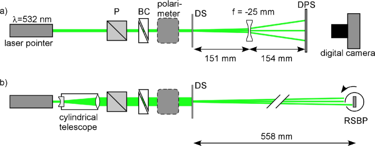
Figure 1: Schemes of the experimental setups used. Abbreviations: P: linear polarizer, DS: double-slit, BC: Babinet compensator, DPS: diffusive projection screen, RSBP: rotating slit beam profiler.

Experiments were performed at the University of Fribourg. Light from a green laser module ($\lambda=532.5$ nm) was sent through a polarizing system consisting of a linear polarizer and a Babinet compensator (BC), which allowed the realization of arbitrary linear and elliptical polarizations (Figs. 1a and b). The beam polarization was measured with a repositionable commercial polarimeter that was removed for the actual diffraction measurements. The double-slit consisted of two 18 mm long slits of 100 $\mu$m, whose centers were separated by 250 $\mu$m. For the experiments shown in Fig. 2, the laser beam has a nearly circular Gaussian intensity profile,

$$I(r)=I_{0}e^{-2r^{2}/w^{2}},$$ (1)

with $w=1.4$ mm.

Two-dimensional interference patterns were recorded with the setup of Fig. 1a for various incident light polarizations. The diffraction patterns were projected onto a thin sheet of paper and their intensity distribution photographed by a digital camera. The results are shown in Fig. 2 for eight circular, elliptical and linear polarization states. In a second experiment, the interference pattern produced by the expanded beam was recorded by a scanning slit beam profiler (Fig. 1b) for eight polarization states. The signal of the beam profiler corresponds to the $x$-dependence of the intensity integrated over the $z$-direction.

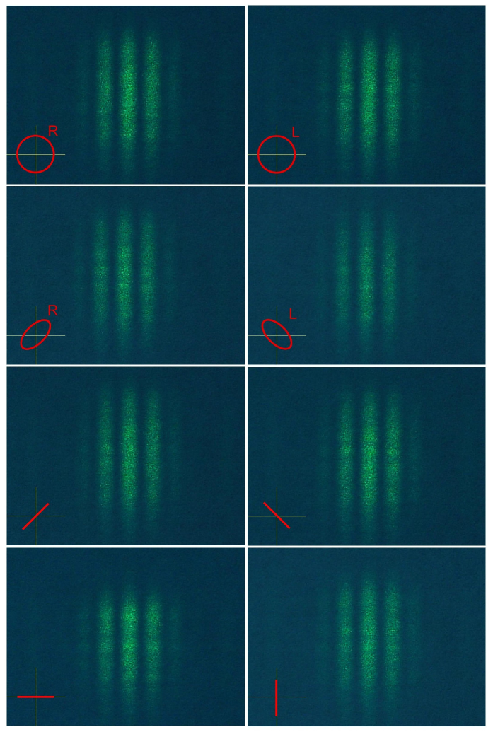
Figure 2: Double-slit interference patterns for eight polarization states of the incident laser light, where insets show right and left circular, right and left elliptic, and linear with angles $\alpha_{p}=45^{\circ},135^{\circ},180^{\circ}$, and $90^{\circ}$.

The results of Fig. 2 seem to indicate a slight polarization dependent transversal shift. This could be traced back to a systematic beam displacement during adjustments of the Babinet compensator. The results of Fig. 3 were obtained after resolving this problem. Fig. 2 —and more convincingly Fig. 3— show that the interference pattern does not depend on the state of polarization of the incident laser light. In a third experiment —carried out with incident circularly polarized light—, we have inserted a horizontal and a vertical polarizer after each slit, respectively. Figure 4 shows the diffraction patterns obtained with and without these polarizers. The peak intensities are in the ratio 4:1, as expected. We note that single photon interference experiments with mutually orthogonally polarized waves are discussed in [11, 12] in the frame of quantum erasure processes.

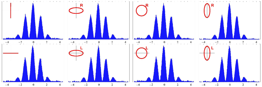
Figure 3: Interference patterns from a double-slit (0.1 mm slit width, separated by 0.25 mm) along the $x$-direction [in mm] obtained from the intensity (EME density) integrated over the $z$-direction for eight polarization states (shown as insets) of the incident light.

Figure 4: Intensity (EME density) as a function of $x$ at the screen behind the double-slit (0.1 mm slit width, separated by 0.25 mm) illuminated with circularly polarized light in two cases: with H and V polarizers (blue curve) just behind each slit and without them (purple curve).

3 Theoretical background

3.1 EM field and EME density behind a double-slit grating for different incident polarizations

Consider the EM field behind a grating situated on the $XZ$-plane, at $y=0$, with slits parallel to the $z$-axis, whose width ($\delta$) is much larger along the $z$-direction than along the $x$-direction. Accordingly, we can assume the EME density to be independent of the $z$-coordinate and, therefore, the electric and magnetic fields will not depend either on this coordinate. As shown in the literature [20], this allows us to express the electric and magnetic fields as a sum of $E$-polarized ($E_{e,x}=E_{e,y}=H_{e,z}=0$) and $H$-polarized ($H_{h,x}=H_{h,y}=E_{h,z}=0$) components, i.e.,

$$\begin{array}[]{l}{\bf E}={\bf E}_{e}+{\bf H}_{h}={\bf E}_{e}+\displaystyle\frac{i}{\omega\epsilon_{0}}\left[\nabla\times{\bf H}_{h}\right],\\ {\bf H}={\bf H}_{e}+{\bf H}_{h}=-\displaystyle\frac{i}{\omega\mu_{0}}\left[\nabla\times{\bf E}_{e}\right]+{\bf H}_{h}.\end{array}$$ (2)

Let us assume that the incident EM field is a plane wave of frequency $\omega$ and wave vector $k$ propagating along the $y$-axis, with arbitrary polarization. It can be written as [15]

$$\begin{array}[]{l}\tilde{\bf E}_{0}({\bf r},t)=\left[-\beta e^{i(ky+\phi)}\hat{\bf x}+\alpha e^{iky}\hat{\bf z}\right]e^{-i\omega t},\\ \tilde{\bf H}_{0}({\bf r},t)=\displaystyle\sqrt{\frac{\epsilon_{0}}{\mu_{0}}}\left[\alpha e^{iky}\hat{\bf x}+\beta e^{i(ky+\phi)}\hat{\bf z}\right]e^{-i\omega t},\end{array}$$ (3)

where $\alpha$, $\beta$ and $\phi$ are real quantities. When $\phi=0$ or $\pi$ and $\alpha$ and $\beta$ are arbitrary, the polarization of the incident wave is linear. If $\phi=\pm\pi/2$ and $\alpha=\beta$, the polarization is circular. In all other cases the polarization is elliptic. In (3) we recognize the $E$-polarized and $H$-polarized components,

$$\begin{array}[]{l}{\bf E}_{0,e}=\alpha\Psi_{0}\hat{\bf z},\\ {\bf H}_{0,h}=\beta\displaystyle\sqrt{\frac{\epsilon_{0}}{\mu_{0}}}\ e^{i\phi}\Psi_{0}\hat{\bf z},\end{array}$$ (4)

with

$$\Psi_{0}({\bf r})=e^{iky}$$ (5)

being the corresponding scalar field satisfying Helmholtz’s equation.

If the boundary conditions at the grating for $E_{e,z}({\bf r})$ and $H_{h,z}({\bf r})$ are the same and both fields satisfy Helmholtz’s equation, we may also assume that these fields are proportional to a scalar field, $\Psi({\bf r})$, which also satisfies the same boundary conditions and the Helmholtz equation. Accordingly, we can express these fields as

$$\begin{array}[]{l}{\bf E}_{e}=\alpha\Psi\hat{\bf z},\\ {\bf H}_{h}=\beta\displaystyle\sqrt{\frac{\epsilon_{0}}{\mu_{0}}}\ e^{i\phi}\Psi\hat{\bf z}.\end{array}$$ (6)

Within the paraxial approximation and for completely transparent slits with their support being totally absorbing, the solution to Helmholtz’s equation behind a double-slit reads as

$$\Psi(x,y)=\sum_{i=1,2}\psi_{i}(x,y)=\displaystyle\sqrt{\frac{k}{2\pi y}}\ e^{-i\pi/4}e^{iky}\sum_{i=1,2}\int_{A}\Psi_{0}(x^{\prime},0^{-})e^{ik(x-x^{\prime})^{2}/2y}dx^{\prime},$$ (7)

where $\Psi_{0}(x^{\prime},0^{-})$ is the incident scalar wave just before the grating. Taking into account (2), (6) and (7), we find that

$${\bf E}={\bf E}_{1}+{\bf E}_{2},\qquad{\bf H}={\bf H}_{1}+{\bf H}_{2},$$ (8)

where

$$\begin{array}[]{l}{\bf E}_{i}=\displaystyle\frac{i\beta e^{i\phi}}{k}\frac{\partial\psi_{i}}{\partial y}\ \hat{\bf x}-\frac{i\beta e^{i\phi}}{k}\frac{\partial\psi_{i}}{\partial x}\ \hat{\bf y}+\alpha\psi_{i}\hat{\bf z},\\ {\bf H}_{i}=\displaystyle-\frac{i\alpha}{\omega\mu_{0}}\frac{\partial\psi_{i}}{\partial y}\ \hat{\bf y}+\frac{i\alpha}{\omega\mu_{0}}\frac{\partial\psi_{i}}{\partial x}\ \hat{\bf y}+\frac{k\beta e^{i\phi}}{\omega\mu_{0}}\ \psi_{i}\hat{\bf z}\end{array}$$ (9)

represent, respectively, the electric and magnetic fields propagating from the $i$th slit, with $=1,2$.

As seen above, experimentally one measures the light intensity, i.e., the EME density on the screen positioned at some distance from the diffraction grating. From the general expression for the EME energy density,

$$U({\bf r})=\displaystyle\frac{1}{4}\left[\epsilon_{0}{\bf E}({\bf r})\cdot{\bf E}^{*}({\bf r})+\mu_{0}{\bf H}({\bf r})\cdot{\bf H}^{*}({\bf r})\right],$$ (10)

we find that the EME density of the incident EM wave (3) is constant (i.e., independent of both $x$ and $y$),

$$U_{0}({\bf r})=\displaystyle\frac{\epsilon_{0}}{2}\left(\alpha^{2}+\beta^{2}\right).$$ (11)

However, as a result of the interaction between the EM field and the grating, the EME density behind this grating becomes dependent on $x$ and $y$,

$$U({\bf r})=\frac{\epsilon_{0}}{4k^{2}}\left(\alpha^{2}+\beta^{2}\right)\left[\left\arrowvert\frac{\partial\Psi}{\partial x}\right\arrowvert^{2}+\left\arrowvert\frac{\partial\Psi}{\partial y}\right\arrowvert^{2}+k^{2}|\Psi|^{2}\right].$$ (12)

The solution (7) to the Helmholtz equation satisfies the approximate relations

$$\left\arrowvert\frac{\partial\Psi}{\partial x}\right\arrowvert\ll\left\arrowvert\frac{\partial\Psi}{\partial y}\right\arrowvert,\qquad\left\arrowvert\frac{\partial\Psi}{\partial y}\right\arrowvert\approx ik\Psi$$ (13)

and, therefore, the EME density (12) becomes proportional to $|\Psi|^{2}$, i.e.,

$$U({\bf r})=\displaystyle\frac{\epsilon_{0}}{2}\left(\alpha^{2}+\beta^{2}\right)|\Psi|^{2}=\frac{\epsilon_{0}}{2}\left(\alpha^{2}+\beta^{2}\right)\left[|\Psi_{1}|^{2}+|\Psi_{2}|^{2}+2{\rm Re}(\psi_{1}\psi_{2}^{*})\right].$$ (14)

As can be noticed from this expression, the $x$ and $y$ dependence of the EME density can be determined through $|\Psi|^{2}$. The polarization of the incident EM wave has no influence on the dependence of the EME density on $x$ and $y$ and, therefore, the interference pattern will be independent of the incident field polarization. This distribution is the same for linear, circular or elliptic polarization, as seen in the experimental results displayed in Figs. 2 and 3. It is important to stress that this conclusion arises from assuming that the EM field does not depend on the $z$-coordinate.

The independence of the EME density on polarization implies that the interference pattern will be the same for both linearly polarized and natural light, in agreement with one of the empirical findings observed by Arago and Fresnel, namely the first Arago-Fresnel law. This law states that “two rays polarized in one and the same plane act on or interfere with each other just as natural rays, so that the phenomena of interference in the two species of light are absolutely the same” [1, 3]. The generalization of this law also includes elliptic polarization, and circular polarization as a special case of elliptic polarization [4].

3.2 EM field and EME density behind a double-slit grating followed by orthogonal polarizers

The approach described above can also be applied to the study of the EM field and EME density behind two slits which are followed by two linear orthogonal polarizers. Now, instead of considering Eqs. (6), the $E$-polarized and $H$-polarized components of the EM field are expressed [15] in terms of $\psi_{1}$ and $\psi_{2}$, as

$$\begin{array}[]{l}{\bf E}_{e}=\alpha\psi_{1}\hat{\bf z},\\ {\bf H}_{h}=\beta\displaystyle\sqrt{\frac{\epsilon_{0}}{\mu_{0}}}\ e^{i\phi}\psi_{2}\hat{\bf z}.\end{array}$$ (15)

Thus, by substituting (15) into (2), we obtain the EM field behind the two slits covered by the orthogonal polarizers,

$$\begin{array}[]{l}{\bf E}_{i}=\displaystyle\frac{i\beta e^{i\phi}}{k}\frac{\partial\psi_{2}}{\partial y}\ \hat{\bf x}-\frac{i\beta e^{i\phi}}{k}\frac{\partial\psi_{2}}{\partial x}\ \hat{\bf y}+\alpha\psi_{1}\hat{\bf z},\\ {\bf H}_{i}=\displaystyle-\frac{i\alpha}{\omega\mu_{0}}\frac{\partial\psi_{1}}{\partial y}\ \hat{\bf y}+\frac{i\alpha}{\omega\mu_{0}}\frac{\partial\psi_{1}}{\partial x}\ \hat{\bf y}+\frac{k\beta e^{i\phi}}{\omega\mu_{0}}\ \psi_{2}\hat{\bf z}.\end{array}$$ (16)

From this EM field, the expression for the EME density will read as

$$U({\bf r}) = \frac{\epsilon_{0}}{2}\ \alpha^{2}\left[\left\arrowvert\frac{\partial\psi_{1}}{\partial x}\right\arrowvert^{2}+\left\arrowvert\frac{\partial\psi_{1}}{\partial y}\right\arrowvert^{2}+k^{2}|\psi_{1}|^{2}\right]+\frac{\epsilon_{0}}{2}\ \beta^{2}\left[\left\arrowvert\frac{\partial\psi_{2}}{\partial x}\right\arrowvert^{2}+\left\arrowvert\frac{\partial\psi_{2}}{\partial y}\right\arrowvert^{2}+k^{2}|\psi_{2}|^{2}\right]$$ (17)

$$\approx \frac{\epsilon_{0}}{2}\left(\alpha^{2}+\beta^{2}\right)\left[|\psi_{1}|^{2}+|\psi_{2}|^{2}\right].$$

Under the presence of orthogonal polarizers behind the slits, the EME density becomes the simple sum of EME densities, which spread out independently from each slit. As a consequence, interference fringes are absent. This is in agreement with the second law experimentally established by Arago and Fresnel [1], namely the second Arago-Fresnel law [3]. This law states that “two rays primitively polarized in opposite planes (i.e., at right angles to each other) have no appreciable action on each other, in the very same circumstances where rays of natural light would interfere so as to destroy each other”. The generalization of this law also includes elliptic and circular polarization of opposite handedness [4].

4 EME-flow-line description

The properties of the EME density behind a grating and the generalized Arago-Fresnel laws may be better understood with the aid of EME flow lines, which can be interpreted as photon trajectories [15]. The equation from which the EME flow lines are obtained is

$$\frac{d{\bf r}}{ds}=\displaystyle\frac{1}{c}\frac{{\bf S}({\bf r})}{U({\bf r})},$$ (18)

where ${\bf S}({\bf r})$ is the real part of the complex Poynting vector,

$${\bf S}({\bf r})=\displaystyle\frac{1}{2}\ {\rm Re}\left[{\bf E}({\bf r})\times{\bf H}^{*}({\bf r})\right],$$ (19)

$U({\bf r})$ is the time-averaged EME density and $s$ is the certain arc-length of the corresponding path. The substitution of Eqs. (7)-(9) into (19) renders the trajectory equations along each direction,

$$\begin{array}[]{l}\displaystyle\frac{dx}{ds}=\frac{i\epsilon_{0}(\alpha^{2}+\beta^{2})}{4kU({\bf r})}\left[\Psi\ \frac{\partial\Psi^{*}}{\partial x}-\Psi^{*}\ \frac{\partial\Psi}{\partial x}\right],\\[11.38092pt] \displaystyle\frac{dy}{ds}=\frac{i\epsilon_{0}(\alpha^{2}+\beta^{2})}{4kU({\bf r})}\left[\Psi\ \frac{\partial\Psi^{*}}{\partial y}-\Psi^{*}\ \frac{\partial\Psi}{\partial y}\right],\\[11.38092pt] \displaystyle\frac{dz}{ds}=-\frac{i\epsilon_{0}\alpha\beta\sin\phi}{2k^{2}U({\bf r})}\left[\frac{\partial\Psi}{\partial x}\frac{\partial\Psi^{*}}{\partial y}-\frac{\partial\Psi}{\partial y}\frac{\partial\Psi^{*}}{\partial x}\right].\end{array}$$ (20)

The projection of the EME flow lines on the $XY$-plane behind a double-slit grating illuminated by circularly polarized laser light, determined from Eqs. (20) and the corresponding experimental conditions, are plotted in Fig. 5. As can be noticed, the EME flow lines (photon trajectories) accumulate according to $U({\bf r})$ [15], as given by Eq. (14). It is important to stress that, in the case of circular and elliptic polarization, EME flow lines do not remain within the $XY$-plane, but there is a flow of energy parcels (photons) along the vertical axis. Nevertheless, the projection of these three-dimensional trajectories onto the $XY$-plane does not depend on the phase angle, $\phi$. Due to this fact, the resulting distribution of end points associated with the trajectories along the x-axis does not depend on polarization. This is consistent with the conclusions derived in the previous section from analysis of the EME density dependence on polarization.

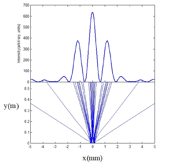
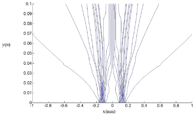
Figure 5: Top: EME density at $L=558$ mm from a double-slit grating illuminated by a circularly polarized laser beam of wavelength $\lambda=532.5$ nm. Centre: 30 EME flow lines behind a double-slit grating determined from (20) and the scalar solution (7) of Helmholtz’s equation. Bottom: Enlargement of the EME flow lines in the near field region. The slits are assumed to be completely transparent, with their support being completely absorbing. The distance between the center of the slits is $d=0.25$ mm and the slit width is $\delta=0.1$ mm.

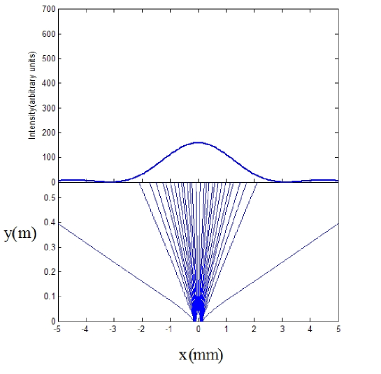
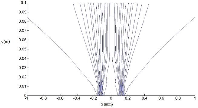
Figure 6: Top: EME density at $L=558$ mm from a double-slit grating with orthogonal polarizers upon the slits and illuminated by a circularly polarized laser beam of wavelength $\lambda=532.5$ nm. Centre: 30 EME flow lines behind a double-slit grating, determined from Eqs. (16), (18) and (19), and the scalar solution (7) of Helmholtz’s equation. Bottom: Enlargement of the EME flow lines in the near field region. The slits are assumed to be completely transparent, with their support being completely absorbing. The distance between the center of the slits is $d=0.25$ mm and the slit width is $\delta=0.1$ mm.

The number of bright and dark fringes obtained in the experiment, where $d=0.25$ mm, $\delta=0.1$ mm and $\lambda=532.5$ nm, agrees fairly well with the corresponding number predicted by the probability amplitude of transverse momenta,

$$c(k_{x})=\displaystyle\frac{1}{\sqrt{2\pi}}\int_{-\infty}^{\infty}dx^{\prime}\Psi(x^{\prime},0^{+})e^{-ik_{x}x^{\prime}}=\frac{1}{\sqrt{2\pi}}\sum_{i=1,2}\int_{A}dx^{\prime}\Psi_{0}(x^{\prime},0^{-})e^{-ik_{x}x^{\prime}},$$ (21)

which, in the case of two slits, is given by

$$c(k_{x})=\frac{2}{\sqrt{\pi\delta}}\frac{\sin(k_{x}\delta/2)}{k_{x}}\ \cos(k_{x}\delta/2).$$ (22)

The centers for the zeroth (central), first ($\pm 1$) and second ($\pm 2$) bright fringes are determined through the relation $\cos(k_{x}\delta/2)=\pm 1$, which renders $k_{x,0}=0$, $k_{x,\pm 1}=\pm 2\pi/d$ and $k_{x,\pm 2}=\pm 4\pi/d$, respectively. On the other hand, the centers of the dark fringes are obtained taking into account that $\cos(k_{x}\delta/2)=0$ and, therefore, $k_{x}=\pm(2n+1)\pi/d$, with $n=0,1,2,\ldots$.

The intensity of the bright fringes decreases because of the envelope of the interference pattern, which is given by first factor and describes the single-slit diffraction. This factor vanishes as $k_{x}$ increases from zero to the value determined by the relation $\sin(k_{x}\delta/2)$, i.e., $k_{x}=\pm 2\pi/\delta$. The point where the intensity falls to zero due to diffraction will coincide with one of the interference minima if

$$\frac{2\pi}{\delta}=\frac{(2n+1)\pi}{d}\quad\longrightarrow\quad\frac{d}{\delta}=\frac{2n+1}{d}.$$ (23)

As seen in the experimental results, this condition holds, because $d/\delta=5/2=2.5$. Therefore, the second bright fringe will be very weak (almost fainting) and the third dark fringe will be negligible in comparison with the remaining continuous dark pattern, as seen in Figs. 2 and 3.

When mutually orthogonal polarizers are positioned upon the slits, both the EME distribution and the EME flow lines change dramatically [15]. The resultant distribution of trajectory end points along the $x$-axis will be consistent with expression (17) for the EME density and interference fringes will be absent.

5 Summary and conclusions: EME flow lines versus “which-slit” information

The analysis presented above throws some novel light on the first and second Arago-Fresnel laws. Moreover, it also results relevant to the discussion on the wave-particle duality of light. The fact that fringes disappear after covering the slits with orthogonal polarizers has been used by the proponents of the principle of complementarity to affirm that information about the path destroys the interference [8, 9]. Within this type of argumentations or interpretations, “path” just means the slit through which the photon passes and any discussion about the whole path, from the grating to the screen, is thus forbidden.

Argumentations based on “which-slit” information are closely related to the reasoning leading to the notion of quantum erasers [8, 9]. By applying this reasoning to the sequence in which the first experiment is a double-slit experiment with orthogonal polarizers and the second experiment is a double-slit experiment without orthogonal polarizers, one could assign the lack of interference to the existence of “which-slit” information. The appearance of interference after removing the polarizers could be then attributed to erasing and, consequently, to the loss of information about the slit which the energy parcel or photon passed through.

The interpretation used here considers a set of entire paths from the grating to the screen, such paths being determined from the EM field and the Poynting vector. EME flow lines starting from slit 1 will end up in the left-hand side part of the screen, while those starting from slit 2 will end up in the right-hand side, as also shown in quantum mechanics for matter particles [28]. This is valid both when interference is present and when no interference fringes are observed [29, 30]. But, the distribution of this EME flow lines is different in the two cases. In the absence of polarizers, the distribution shows interference fringes (Fig. 5); in the presence of polarizers, the fringes are absent (Fig. 6), in perfect agreement with experimental results shown at Fig. 4. Hence, observer’s information about the slit through which photon (energy parcel) went through is not relevant for the existence of interference. What is relevant it is the form of the EME field and its corresponding form, which will model consequently the distribution of trajectories and their topology.

References

- [1] D. F. J. Arago and A. J. Fresnel, “Memoir on the action of rays of polarized light upon each other”, Ann. Chimie Physique, 288 (1819).
- [2] M. Henry, Am. J. Phys., 49, 690 (1981).
- [3] R. Barakat, J. Opt. Soc. Am. A, 10, 180 (1993).
- [4] M. Mujat, A. Dugariu, and E. Wolf, J. Opt. Soc. Am. A, 21, 2414 (2004).
- [5] J. L. Hunt and G. Karl, Am. J. Phys., 38, 1249 (1970).
- [6] D. Pescetti, Am. J. Phys., 40, 735 (1972).
- [7] B. Kanseri, N. S. Bisht, H. C. Kandpal, and S. Rath, Am. J. Phys., 76, 39 (2008).
- [8] M. O. Scully, B. G. Englert, and H. Walter, Nature, 351, 111 (1991).
- [9] S. P. Walborn, M. O. Terra-Cunha, S. Padua, and C. H. Monken, Phys. Rev. A, 65, 033818 (2002).
- [10] T. L. Dimitrova and A. Weis, Am. J. Phys., 76, 137 (2008).
- [11] T. L. Dimitrova and A. Weis, Phys. Scr., T135, 014003 (2009).
- [12] T. L. Dimitrova and A. Weis, Eur. J. Phys., 31, 625 (2010).
- [13] A. Tonomura, J. Endo, T. Matsuda, T. Kawasaki, and H. Ezawa, Am. J. Phys., 57, 117 (1989).
- [14] F. Shimuzu, K. Shimuzu, and H. Takuma, Phys. Rev. A 46, R17 (1992).
- [15] A. S. Sanz, M. Davidović, M. Božić, and S. Miret-Artés, Ann. Phys., 325, 763 (2010).
- [16] I. Bialynicki-Birula, Prog. Opt., 36, 245 (1996).
- [17] R. Fedele and M. A. Man’ko, Eur. Phys. J. D, 27, 263 (2003).
- [18] M. Man’ko, Eur. Phys. J.-Spec. Topics, 160, 269 (2008).
- [19] W. Braunbek and G. Laukien, Optik, 9, 174 (1952).
- [20] M. Born and E. Wolf, Principles of Optics, 7th ed., Pergamon Press, Oxford (2002).
- [21] R. D. Prosser, Int. J. Theor. Phys., 15, 169 (1976).
- [22] R. D. Prosser, Int. J. Theor. Phys., 15, 181 (1976).
- [23] R. D. Prosser, “Infinite wave resolution of the EPR paradox”, in: Open Questions in Quantum Physics, G. Tarozzi and A. van der Merwe (eds.), D. Reidel Publishing Company, Boston (1985), pp. 119-127.
- [24] M. Davidović, A. S. Sanz, D. Arsenović, M. Božić, and S. Miret-Artés, Phys. Scr., T135, 014009 (2009).
- [25] D. Arsenović, M. Božić, O. V. Man’ko, and V. I. Man’ko, J. Russ. Laser Res., 26, 94 (2005).
- [26] M. Gondran and A. Gondran, hal.archives-ouvertes.fr/hal-00416055, version 1 - 11 Sep 2009.
- [27] A. J. Fresnel, “Memoir on the diffraction of light”, in: Oeuvres Completes, Imprimerie imperiale, Paris (1866), tome 1, pp. 254-255 [reprinted in: H. Crew (ed.), The Wave Theory of Light. Memoirs by Huygens, Young and Fresnel, American Book Company, New York (1900).
- [28] A. S. Sanz and S. Miret-Artés, J. Phys. A 41, 435303 (2008).
- [29] A. S. Sanz and F. Borondo, Eur. Phys. J. D 44, 319 (2007).
- [30] A. S. Sanz and F. Borondo, Chem. Phys. Lett., 478, 301, (2009).