Strong coupling superconductivity mediated by three-dimensional anharmonic phonons

Abstract

We investigate three-dimensional anharmonic phonons in tetrahedral symmetry and superconductivity mediated by these phonons. Three-dimensional anharmonic phonon spectra are calculated directly by solving Schrödinger equation and the superconducting transition temperature is determined by using the theory of strong coupling superconductivity assuming an isotropic gap function. With increasing the third-order anharmonicity $b$ of the tetrahedral ion potential, we find a crossover in the energy spectrum to a quantum tunneling regime. We obtain strongly enhanced transition temperatures around the crossover point. We also investigate the anharmonic effects on the Debye-Waller factor, the phonon spectral functions and the density profile, as a function of the anharmonicity $b$ and temperature. The isomorphic first-order transition observed in KOs₂O₆ is discussed in terms of the first excited state energy $\Delta$, and the coupling constant $\lambda$ in the strong coupling theory of superconductivity. Our results suggest the decrease in $\lambda$ and increase in $\Delta$ below the first order transition temperature. We point out that the change in the oscillation amplitude $\langle x^{2}\rangle$ and $\langle xyz\rangle$ characterizes this isomorphic transition. The chemical trends of the superconducting transition temperature, $\lambda$, and $\Delta$ in the $\beta$-pyrochlore compounds are also discussed.

I Introduction

Recently, various low-energy properties arising from anharmonic ion oscillations have attracted much attention. An ion located at the center of an over-sized cage oscillates with large amplitude and thus the anharmonic terms in the potential energy play an important role. Indeed, these anharmonic oscillations are observed in $\beta$-pyrochlore,HiroiUnprecedented ; Hiroi2ndAno ; SummaryHiroi ; Hasegawa filled-skutterudite,Goto ; Kaneko ; Kotegawa and clathrate compounds. Sales ; Zerec ; Matsumoto In metallic systems, such anharmonic oscillations interact with conduction electrons, and due to their large amplitude, the electron-phonon coupling constant becomes large. The large anharmonicity and the strong electron-phonon coupling lead unusual relaxation of conduction electrons,SummaryHiroi ; ThermalCondKasahara anomalous nuclear magnetic relaxation time,Yoshida ; Nakai the sound velocity anomalies,Goto ; Nemoto ; Ishii ; Nakanishi and the strong coupling superconductivity.BattloggSC ; IsotropicGappSCSC ; peneShimono ; SummaryHiroi ; Nagao ; Thalmeier ; Chang

These anharmonic oscillations in these systems have also been studied theoretically. Dahm and Ueda discussed the anomalous temperature dependence of the resistivityHiroiUnprecedented ; Hiroi2ndAno ; SummaryHiroi and the NMR relaxation timeYoshida observed in KOs₂O₆ by using a single-site anharmonic phonon model, employing the self-consistent Gaussian approximation for the quartic term of the ion displacement.DahmUeda Recently, Yamakage and Kuramoto extended this approach to the lattice problem in the same level of Gaussian approximation.Yamakage These works can explain the softening of optical-phonon frequency as temperature decreases observed in many compounds.Hasegawa ; Matsumoto ; NeutronSasai ; Galati ; Mukta

The anharmonic ion oscillations had been discussed also as a possible mechanism of high transition temperature superconductivity, particularly for high $T_{\rm c}$ cuprates.Plakida ; Hardy ; Crespi ; MahanSofo As for the systems of anharmonic ion oscillations in over-sized cages, importance of contributions of low-energy Pr ion oscillations to the superconductivity is pointed out in PrOs₄Sb₁₂.Thalmeier Recently, Chang, et al.,Chang discussed the superconductivity in KOs₂O₆ using strong coupling theory of $s$-wave superconductivityManalo also employing the Gaussian approximationDahmUeda for anharmonicity.

In this paper, we focus on the $\beta$-pyrochlore compounds $A$Os₂O₆ ($A$=K, Rb, or Cs). Monovalent $A$-cations are located at the center of the Os₁₂O₁₈ cages and form a diamond lattice structure. Lattice dynamics was investigated by neutron-scattering experiments,NeutronSasai ; Galati ; Mukta and a low-energy optical phonon is observed at about 3 meV in the K compound. This is basically K-cation oscillations, and the same phonon is also observed at around 5-7 meV in the Rb and Cs compounds. The root-mean-square amplitude of the K oscillation turns out to be 0.12-0.14 Å at zero temperature from the elastic neutron scatteringNeutronSasai ; Galati while much smaller values are reported for Rb and Cs compounds.NeutronSasai

The first-principle calculations indicate that the K ion potential has large anharmonicity and is very shallow along [111] and three other equivalent directions.BandCal It is also calculated that the first excited state has the excitation energy of $\sim$8 K and K-cation oscillation amplitude is as large as 1 Å at zero temperature. These values are quite different from the experimental data, indicating that some parameters in the ion potential are not so realistic. In the present paper, we will first systematically analyze the effects of anharmonicity of the ion potential on the ion dynamics in KOs₂O₆.

The $\beta$-pyrochlore compounds reveal superconducting phase transition and the transition temperature $T_{\rm c}$’s are 9.6 K, 6.3 K and 3.3 K for $A$=K, Rb, and Cs, respectively. These values of $T_{\rm c}$ are inversely related to the $A$-cation size, i.e., $T_{\rm c}$ is the highest for the smallest ion: potassium. The symmetry of the gap function is considered to be fully gapped $s$-wave.Yoshida ; IsotropicGappSCSC ; peneShimono It has been also shown that the electron-phonon coupling is large.SummaryHiroi ; IsotropicGappSCSC ; Nagao Thus, it is expected that the conduction electrons on the cages strongly interact with the anharmonic oscillations of ion inside the cage in these systems.

For KOs₂O₆, in addition to superconducting transition, there exists a first-order structural transition at $T_{p}=7.5$ K. At this transition, no sign of symmetry breaking has been observed.SummaryHiroi ; Hasegawa The oscillation of K-cation seems less anharmonic below $T_{p}$ as indicated by electrical resistivity, specific heat jump at $T_{\rm c}$ in magnetic fields and the mean free path estimated from the upper critical field $H_{c2}$.SummaryHiroi Recently, we have proposed that this is driven by a sudden change in K-cation oscillation amplitude driven by intersite ion interactions.Hat The amplitude of the low-energy excited state with $xyz$ symmetry jumps at $T_{p}$, but this does not change the $T_{d}$ point-group symmetry.

The main purpose of this paper is to clarify the properties of anharmonic oscillations in tetrahedral symmetry, which is the local symmetry for $A$-cations in $A$Os₂O₆, and the superconductivity mediated by these anharmonic oscillations. In order to fully take into account the anharmonicity and anisotropy, we will solve the three-dimensional Schrödinger equation for an anharmonic oscillator in the tetrahedral symmetry. Using these exact phonon eigenstates, we will then discuss the strong coupling superconductivity assuming an $s$-wave pairing.

This paper is organized as follows. In Sec. II, we will calculate the energy spectrum of the anharmonic potential problem and discuss various thermodynamic and dynamical quantities and their dependence on temperature. Anharmonic effects on Debye-Waller factor will also be discussed. Section III is devoted to the discussions for strong coupling superconductivity mediated by the anharmonic ion oscillations discussed in Sec. II. In Sec. IV, we will discuss the relevance of the present results to the $\beta$-pyrochlore compounds. We also apply our theory to discuss the changes in phonon dynamics at the first-order transition at $T_{p}$. Finally Sec. V is a summary of this paper.

II Anharmonic phonons

II.1 Model

In this paper, we investigate an anharmonic oscillation of K ion in KOs₂O₆. Our model is anharmonic local phonons at each lattice point and we assume the local symmetry is tetrahedral one which corresponds to the case of K-site symmetry in KOs₂O₆. In tetrahedral symmetry, in addition to spherical and cubic fourth order terms, there exists a third-order anharmonic term which breaks inversion symmetry and the Hamiltonian is given by

$$H = -\frac{\hbar^{2}}{2M}\nabla^{2}_{\bf R}+V({\bf R}),$$ (1)

$$V(\bf R) = \frac{1}{2}M\Omega^{2}_{0}|{\bf R}|^{2}+BXYZ$$ (2)

$$+C_{1}|{\bf R}|^{4}+C_{2}(X^{4}+Y^{4}+Z^{4}),$$

where ${\bf R}=(X,Y,Z)$ is the real-space displacement of the ion from the equilibrium position. $M$ is the mass of the ion. Throughout this paper we set $M/m_{e}=71748$, where $m_{e}$ is the mass of electron, except for discussions in Sec. IV.1, and this corresponds to the mass of K ion. $\Omega_{0}$ and $B$ are coefficients of second- and third-order terms in the ion potential, while $C_{1}$ and $C_{2}$ are isotropic and cubic fourth-order terms, and we ignore the higher-order potential terms of $O(R^{5})$. To study dependence on potential parameters, it is useful to rewrite Hamiltonian (1) into a dimensionless form by renormalizing displacement and energy by their units. As for the energy unit, we choose the energy of harmonic phonon corresponding the second-order term $\hbar\Omega_{0}$. The unit of the length is chosen as $a_{0}\equiv\hbar/M\Omega_{0}=a_{B}\sqrt{2(e^{2}/2a_{B})(m_{e}/M)/\hbar\Omega_{0}}$. Here, $a_{B}$ is the Bohr radius $a_{B}=\hbar^{2}/m_{e}e^{2}\simeq 0.53$ Å.

In these units, Hamiltonian (1) is transformed to

$$\bar{H} \equiv \frac{H}{\hbar\Omega_{0}}=-\frac{1}{2}\nabla^{2}_{\bf r}+\bar{V}(\bf r),$$ (3)

$$\bar{V}(\bf r) = \frac{1}{2}\omega_{0}|{\bf r}|^{2}+bxyz+c_{1}|{\bf r}|^{4}+c_{2}(x^{4}+y^{4}+z^{4}),$$ (4)

where ${\bf r}=(x,y,z)={\bf R}/a_{0}$. $b$ and $c_{1}$ and $c_{2}$ are dimensionless constants and $\omega_{0}$ is introduced to vary the second-order term for later purpose, but $\omega_{0}=1$ for the main part of this paper. In Secs. III and IV, we will use different values of $\omega_{0}$ to examine the effects of changes in the second-order term.omega0var Throughout this paper we set $\hbar\Omega_{0}=44$ K which corresponds to the energy scale of the optical-phonon frequency observed in $\beta$-pyrochlore compounds,SummaryHiroi ; NeutronSasai ; Mukta and thus $a_{0}\simeq a_{B}/\sqrt{10}$.

In the limit of $b=c_{1}=c_{2}=0$, Hamiltonian (3) can be diagonalized by using creation and annihilation operators as,

$$\bar{H} = a_{x}^{\dagger}a_{x}+a_{y}^{\dagger}a_{y}+a_{z}^{\dagger}a_{z}+\frac{3}{2},$$ (5)

where $a_{\mu}\equiv\frac{1}{\sqrt{2}}(\partial_{\mu}+x_{\mu})$ with $\mu=x$, $y$ or $z$. Eigenstates are labeled by three occupation numbers as $\bar{H}|n_{x},n_{y},n_{z}\rangle=(n_{x}+n_{y}+n_{z}+3/2)|n_{x},n_{y},n_{z}\rangle$ and $a^{\dagger}_{\mu}a_{\mu}|n_{x},n_{y},n_{z}\rangle=n_{\mu}|n_{x},n_{y},n_{z}\rangle$.

For nonzero $b$, $c_{1}$, and $c_{2}$, we diagonalize Hamiltonian (3) numerically in the restricted Hilbert space spanned by $\{|n_{x},n_{y},n_{z}\rangle\}$ with $n_{x}+n_{y}+n_{z}\leq n_{\rm max}$. In this paper, we use $n_{\rm max}=40$ which corresponds to the Hilbert space with 12341 states and check the convergence by comparing the results for $n_{\rm max}=50$ including 23426 states. We employ this approach rather than the conventional self-consistent Gaussian approximationDahmUeda ; Yamakage . This is because the conventional approximation does not work for the potential, Eq. (4) since the third-order term cannot be decoupled as in the fourth-order terms. It is also important that, as will be shown later, energy differences between adjacent eigenstate multiplets are not the same, and this property cannot be described by the self-consistent Gaussian approximation.

II.2 Energy spectrum

In Fig. 1, we show a low-energy part of the energy spectra of Hamiltonian (3) as a function of the third-order anharmonicity $b$ for $c_{1}=0.04$ and $c_{2}=0.01$. The ground state is always nodeless in the space ${\bf r}$ and therefore singlet, while the first excited states are triplet, corresponding to $s$ and $p$ orbitals for the case of isotropic potential. As $b$ increases, the energy of the lowest singlet excited state (hereafter, this state will be referred to as $s^{\prime}$ state) decreases and shows an anticrossing with the ground state at $b=b^{*}\sim 1.7$. This kind of anti-crossing behavior does not occur in the one-dimensional anharmonic potential problem: $V(X)=aX^{2}+bX^{4}$.DahmUeda ; Matsumoto Interestingly, near $b=b^{*}$ the five lowest-energy states are well separated from other states in the energy spectra. Thus, the validity of our previous five-state toy model is justified around this crossover region.Hat

For $b>b^{*}$, the excited triplet states, which are $p$-wave like, are nearly degenerate with the ground state. This means that these four states are localized away from the origin in the four directions: $[\bar{1}\bar{1}\bar{1}]$, $[11\bar{1}]$, $[\bar{1}11]$, and $[1\bar{1}1]$. For the illustration, we show the potential form along $[100]$, $[110]$, and $[111]$ directions in Fig.2. It is clear that an off-center potential local minimum emerges along [111] direction as $b$ increases. The energy of the first excited state from the ground state $\Delta$ is small, owing to smallness of the quantum tunneling probability between different valleys. These four states form $sp^{3}$ orbitals and their energy can be well described by considering the quantum tunneling of the ion between the four potential minimum positions. Hereafter, we call these states in this parameter region ($b>b^{*}$) as quantum tunneling states.

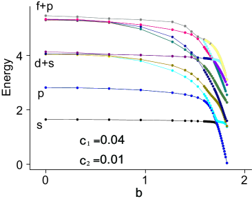
Figure 1: (Color online) Energy eigenvalues vs the third-order anharmonic parameter $b$ for $c_{1}=0.04$ and $c_{2}=0.01$. $s$, $p$, $d$, and $f$ denote the approximate orbital symmetry, which is exact in the isotropic harmonic potential case.

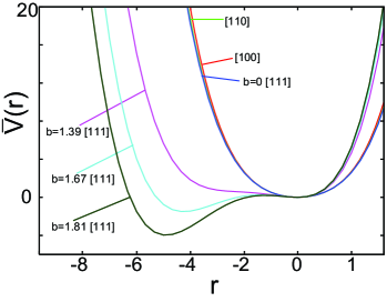
Figure 2: (Color online) Potential along [100], [110], and [111] directions for various $b$. $c_{1}=0.04$ and $c_{2}=0.01$. ${\bf r}=r{\bf n}$, where $\bf n$ being the unit vector along each direction.

II.3 Observables

We now investigate the temperature dependence of the oscillation amplitude of these anharmonic ions. Thermodynamic average of observable $A$ is calculated by the formula:

$$\langle A\rangle = \sum_{n}w_{n}\langle n|A|n\rangle,$$ (6)

where $|n\rangle$ is the eigen state of Hamiltonian (1) with eigenenergy $E_{n}$ and $w_{n}$ is its Boltzmann weight $w_{n}=\exp(-E_{n}/T)/\sum_{m}\exp(-E_{m}/T)$, and $T$ is the temperature. In the summation in Eq. (6), we discard states with $E_{n}>0.8n_{\rm max}\omega_{0}$, since the high-energy parts of our energy spectrum is not correct due to the cutoff $n_{\rm max}$ and the high-energy part does not matter as long as the low-temperature properties of the system are concerned.

In Fig 3, we show the temperature dependence of fluctuations $\langle x^{2}\rangle=\langle{\bf r}^{2}\rangle/3$ and $\langle xyz\rangle$. Note that since $xyz$ is invariant quantity in tetrahedral symmetry, this does not vanish except for $b=0$. As the temperature decreases, both $\langle x^{2}\rangle$ and $|\langle xyz\rangle|$ decrease and saturate to finite values for $b<b^{*}$. On the other hand, for $b>b^{*}$, these quantities increase at low temperatures suggesting the quantum tunneling state.

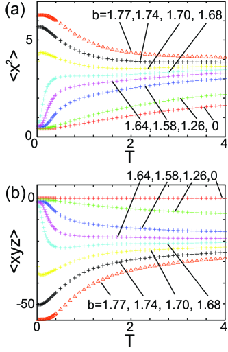
Figure 3: (Color online) Temperature dependence of thermodynamic average (a) $\langle x^{2}\rangle$ and (b) $\langle xyz\rangle$. $c_{1}=0.04$ and $c_{2}=0.01$.

To see the change with $b$ more clearly, we calculate the ion density $\rho({\bf r})\equiv\sum_{n}w_{n}|\Psi_{n}({\bf r})|^{2}$ at position ${\bf r}$. Here ${\Psi_{n}({\bf r})}$ is the wave function at position ${\bf r}$ which is normalized as $\int d^{3}x|\Psi_{n}({\bf r})|^{2}=1$. In Figs. 4(a)-4(d), we show $\rho(\bf r)$ along [111] direction, ${\bf r}=r(1,1,1)/\sqrt{3}$, for several temperatures. $\rho({\bf r})$ in other directions has monotonic temperature dependence and is peaked at ${\bf r}=(0,0,0)$ as in Fig. 4(a). As $b$ increases, a part of the weight of $\rho(\bf r)$ shifts to the position around $r\sim-4$. Interestingly near $b=b^{*}$ [Fig. 4(c)], the temperature dependence of $\rho(\bf r)$ at $r\sim-4$, is non-monotonic, i.e., as $T$ decreases, $\rho(-4)$ increases first, but decreases below $T\sim 0.3\sim\Delta$. In Fig. 4(d), the $\rho(0)$ is suppressed at low temperatures reflecting the nature of the quantum tunneling states, since the potential minimum away from the origin is deep enough as shown in Fig. 2.

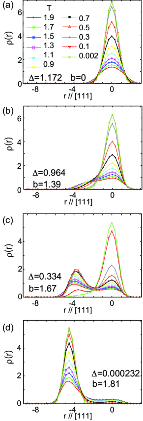
Figure 4: (Color online) Atomic density profile $\rho({\bf r})$ along ${\bf r}=r(1,1,1)/\sqrt{3}$ for various $b$. $c_{1}=0.04$ and $c_{2}=0.01$.

II.4 Debye-Waller factor

Now we discuss the Debye-Waller factor, which contains information about the amplitude of ion oscillation and it is observed by elastic neutron-scattering experiments.NeutronText Consider an atom whose position is represented by $\bf d$ in a unit cell and denote its displacement by ${\bf u_{d}}=(u_{\bf d}^{x},u_{\bf d}^{y},u_{\bf d}^{z})$. Then, the Debye-Waller factor at the scattering wave vector ${\bf Q}$ for this atom $e^{-W_{\bf d}({\bf Q})}$ is given by

$$\exp[-W_{\bf d}({\bf Q})]=\langle\exp(-i{\bf Q\cdot u_{d}})\rangle.$$ (7)

In the harmonic approximation, Eq. (7) reduces to

$$W_{\bf d}^{(2)}({\bf Q})=\frac{1}{2}\langle({\bf Q\cdot u_{d}})^{2}\rangle.$$ (8)

Using $W_{\bf d}(\bf Q)$, the static structure factor $F(\bf Q)$ is represented as

$$F({\bf Q}) = \sum_{\bf d}\bar{b}_{\bf d}\exp(i{\bf Q\cdot d})\exp[-W_{\bf d}({\bf Q})],$$ (9)

where $\bar{b}_{\bf d}$ is the averaged scattering length of the atom at position ${\bf d}$.

When anharmonicity is not negligible, Eq. (8) is not sufficient and we must take into account higher-order terms. Up to the third order in $(\bf Q\cdot u_{d})$, we obtain

$$W^{(3)}_{\bf d}({\bf Q})=\frac{1}{2}\langle({\bf Q\cdot u_{d}})^{2}\rangle+\frac{i}{6}\langle({\bf Q\cdot u_{d}})^{3}\rangle.$$ (10)

As an example, let us consider K atoms in KOs₂O₆, which constitute a diamond sub-lattice. There are two sites in the unit cell, ${\bf d}_{A}=(0,0,0)$ and ${\bf d}_{B}=\frac{a}{4}(1,1,1)$. Here $a$ is the lattice constant. From the symmetry arguments, we obtain

$$\frac{1}{2}\langle({\bf Q\cdot u_{d}})^{2}\rangle = \frac{1}{6}|{\bf Q}|^{2}\langle|{\bf u_{d}}|^{2}\rangle\equiv W^{\prime}_{\bf d},$$ (11)

$$\frac{1}{6}\langle({\bf Q\cdot u_{d}})^{3}\rangle = Q_{x}Q_{y}Q_{z}\langle u_{\bf d}^{x}u_{\bf d}^{y}u_{\bf d}^{z}\rangle\equiv W^{\prime\prime}_{\bf d}.$$ (12)

In the diamond lattice structure, $W^{\prime}_{{\bf d}_{A}}({\bf Q})=W^{\prime}_{{\bf d}_{B}}({\bf Q})\equiv W^{\prime}({\bf Q})$ and $W^{\prime\prime}_{{\bf d}_{A}}({\bf Q})=-W^{\prime\prime}_{{\bf d}_{B}}({\bf Q})\equiv W^{\prime\prime}({\bf Q})$. Using Eqs. (11) and (12) and setting $\bar{b}\equiv\bar{b}_{{\bf d}_{A}}=\bar{b}_{{\bf d}_{B}}$, we obtain

$$|F({\bf Q})|^{2} = 2\bar{b}^{2}\exp[-2W^{\prime}({\bf Q})]$$ (13)

$$\times \Bigg{\{}1+{\rm cos}\Big{[}{\bf Q}\cdot({\bf d}_{A}-{\bf d}_{B})-2W^{\prime\prime}({\bf Q})\Big{]}\Bigg{\}}.$$

Thus, the effective $W({\bf Q})$ becomes

$$W_{\rm eff}({\bf Q}) = W^{\prime}({\bf Q})-\frac{1}{2}\log 2$$

$$- \log\Big{|}{\rm cos}\Big{[}\frac{1}{2}{\bf Q}\cdot({\bf d}_{A}-{\bf d}_{B})-W^{\prime\prime}({\bf Q})\Big{]}\Big{|}.$$

It is important to note that since the $W^{\prime\prime}({\bf Q})$ depends on the wave vector as $Q_{x}Q_{y}Q_{z}$, the effect of anharmonicity is anisotropic. For example, at ${\bf Q}_{111}=(1,1,1)2\pi/a$, $W_{\rm eff}$ is given by

$$W_{\rm eff}({\bf Q}_{111}) = W_{\rm eff}(-{\bf Q}_{111}),$$

$$= W^{\prime}({\bf Q}_{111})-\frac{1}{2}\log\Bigg{\{}1+{\rm sin}\Big{[}2W^{\prime\prime}({\bf Q}_{111})\Big{]}\Bigg{\}},$$

whereas at ${\bf Q}_{200}=(2,0,0)2\pi/a$, we obtain

$$W_{\rm eff}({\bf Q}_{200})=W^{\prime}({\bf Q}_{200})=\frac{4}{3}W^{\prime}({\bf Q}_{111}).$$ (16)

The third-order contribution $\langle u_{\bf d}^{x}u_{\bf d}^{y}u_{\bf d}^{z}\rangle$ also modifies the extinction rule of the structure factor. According to Eq. (13), $|F({\bf Q})|^{2}=0$ at ${\bf Q}=(2,0,0)2\pi/a$ and also at $(2,2,2)2\pi/a$ due to the interference factor $1+\cos[{\bf Q}\cdot({\bf d_{A}-d_{B}})]$ when $W^{\prime\prime}({\bf Q})$ is set to be zero. For $b\neq 0$, $\langle u_{\bf d}^{x}u_{\bf d}^{y}u_{\bf d}^{z}\rangle$ is finite and this leads to nonvanishing $W^{\prime\prime}({\bf Q})$ at ${\bf Q}=(2,2,2)2\pi/a$ but $W^{\prime\prime}({\bf Q})=0$ at ${\bf Q}=(200)2\pi/a$, since $W^{\prime\prime}({\bf Q})$ is proportional to $Q_{x}Q_{y}Q_{z}$. Therefore, $|F({\bf Q})|^{2}$ is nonvanishing at ${\bf Q}=(2,2,2)2\pi/a$ while remains zero at ${\bf Q}=(2,0,0)2\pi/a$.

We show the calculated $W_{\rm eff}({\bf Q}_{111})$ for several values of $b$ as a function of temperature in Fig. 5. In Fig. 5(a), the first term in Eq. (LABEL:W111) is shown and $W_{\rm eff}({\bf Q}_{111})$ for $b>0$ and $b<0$ are shown in (b) and (c), respectively. It is easily seen that, for small $b$, $W_{\rm eff}({\bf Q}_{111})$ in Figs. 5(b) and 5(c) are essentially the same as $W^{\prime}({\bf Q}_{111})$ in (a), while, for larger $b$, $W_{\rm eff}({\bf Q}_{111})$ is enhanced (suppressed) for $b>0$ in (b) [$b<0$ in (c)]. For other directions of ${\bf Q}$ with $Q_{x}Q_{y}Q_{z}=0$, $W_{\rm eff}({\bf Q})$ does not include the contribution of the third order term $W^{\prime\prime}(\bf Q)$ and thus, $W_{\rm eff}=W^{\prime}$.

Figure 6 shows the wave-vector dependence of $|F({\bf Q})|^{2}$ for several temperatures and $b$. Note that $F(\bf Q)$ at ${\bf Q}=(2,0,0)2\pi/a$ vanishes due to the extinction rule mentioned above, while the intensity at ${\bf Q}=(2,2,2)2\pi/a$ appears for nonzero $b$ although its strength is weak. Concerning $b$ dependence, $|F({\bf Q})|^{2}$ for $b=1.74$ is much suppressed for large $|{\bf Q}|$ and low temperatures, which is originated from the large displacement for $b>b^{*}$. As for the temperature dependence, $|F({\bf Q})|^{2}$ increases as $T$ decreases for $b=0$ and $1.58$, while decreases for $b=1.74>b^{*}$. This temperature dependence of $|F({\bf Q})|^{2}$ for $b>b^{*}$ is also understood from the temperature dependence of $W_{\rm eff}$ in Fig. 5, where $W_{\rm eff}$ for larger $b>b^{*}$ increases as $T$ decreases.

We note that by careful analysis of the neutron data, as we have demonstrated the effects of the third-order term on the Debye-Waller factor, we can obtain useful information about anharmonicity in the real materials. In KOs₂O₆, since there are a lot of kinds of atoms such as the oxygen and osmium, our results presented in this section cannot directly be compared with the neutron data of KOs₂O₆. It is desired to carry out high resolution neutron scattering experiments using the single crystal and analyze the results by taking into account the anharmonicity.

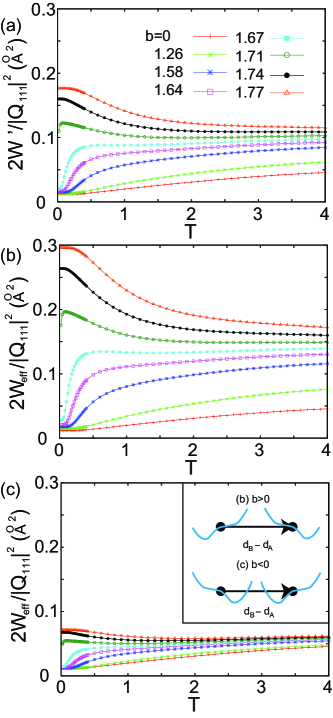
Figure 5: (Color online) Temperature dependence of the exponent of the Debye-Waller factor for $c_{1}=0.04$ and $c_{2}=0.01$. (a) $W^{\prime}({\bf Q}_{111})$. (b) $W_{\rm eff}({\bf Q}_{111})$ for $b>0$. (c) $W_{\rm eff}({\bf Q}_{111})$ for $b<0$. Inset in (c): schematic potential form along the [111] direction in (b) and (c) for large $b$ cases.

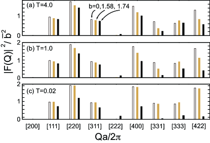
Figure 6: (Color online) ${\bf Q}$ dependence of $|F({\bf Q})|^{2}$ for $c_{1}=0.04$ and $c_{2}=0.01$ at temperatures (a) $T=4.0$, (b) $T=1.0$, and (c) $T=0.02$. For each of ${\bf Q}$, $|F({\bf Q})|^{2}$ values for $b=0$, $1.58$, and $1.74$ are shown from left to right. For ${\bf Q}=2\pi(2,0,0)/a$, $|F({\bf Q})|^{2}$ is always zero.

II.5 Ion dynamics

Now let us investigate the dynamics of the anharmonic ion oscillation. In Fig. 7, we show the phonon density of states (DOS) $F(\omega)$, which is calculated from the correlation function $D$,

$$D_{\mu\mu^{\prime}}(\omega) = \sum_{nm}(w_{n}-w_{m})\frac{\langle n|x_{\mu}|m\rangle\langle m|x_{\mu^{\prime}}|n\rangle}{\omega-E_{m}+E_{n}+i\eta}.$$ (17)

The DOS is given by its imaginary part, $F(\omega)=-{\rm Im}D_{xx}(\omega)/\pi$. Notice $D_{xx}(\omega)=D_{yy}(\omega)=D_{zz}(\omega)$ in the tetrahedral symmetry. We set the phenomenological broadening parameter $\eta=0.26$. Although one can try more sophisticated analyses by introducing dissipation by electron-phonon couplings or couplings with other degrees of freedom to calculate the imaginary part of the self-energy $\eta(\omega)$,Hat2 ; Takechi it is sufficient at this stage to restrict ourselves in the phenomenological level as long as characteristic properties of the DOS are concerned.

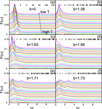
Figure 7: (Color online) Phonon DOS $F(\omega)$ for various $b$’s fixing $c_{1}=0.04$ and $c_{2}=0.01$. The data correspond to $T=$10, 9.2, 8.4, 7.6, 6.8, 6.0, 5.2, 4.4, 3.6, 2.8, 2.0, 1.8, 1.6, 1.4, 1.2, 1.0, 0.8, 0.6, 0.4, 0.2, and 0.1, from bottom to top and each curve is shifted up by 0.005. Energy eigenvalues relative to the energy of the ground state are shown by short bars in each panel.

Figure 7(a) shows the phonon DOS $F(\omega)$ for the case $b=0$ and the eigenenergies relative to the ground state energy indicated by small bars. It is clearly seen that the position of the peak decreases as the temperature decreases and this softening is consistent with the study based on self-consistent Gaussian approximations.DahmUeda ; Yamakage The single peak in $F(\omega)$ is actually constituted of many Lorentzian peaks each of which has a width of $\eta=0.26$. In this case of $b=0$, the transition matrix elements are sizable only between neighboring “multiplets” of the corresponding harmonic system. Because of the fourth-order anharmonicity, $c_{1}$ and $c_{2}$, the degeneracy of each multiplet is only approximate and slightly lifted, and also the energy separation between multiplets increases with increasing energy. Since the distribution of Lorentzian peak positions is quite smooth and the energy dependence of Boltzmann weight is monotonic, they finally form a single broad peak. Its position shifts from a low energy at low $T$ where only the ground state is an important initial state to a higher energy at higher $T$ where higher excited states contribute more importantly.

For $b>0$, qualitatively different behaviors appear as shown in Figs. 7(b)-7(f). The transition matrix elements are now finite for many more pairs of eigenstates $\langle n|x|m\rangle$ for nonzero $b$. This is because the point-group symmetry changes from cubic $O_{h}$ to tetrahedral $T_{d}$ and the eigenstates $|n\rangle$ do not have definite parity related to inversion symmetry ${\bf r}\to-{\bf r}$. In this point-group symmetry, for example, $x$ and $yz$ are bases of the same $T_{2}$ irreducible representation. As a result, the matrix element such as $\langle yz|x|s\rangle$ is nonvanishing (here “$s$” means an isotropic $s$-wave state, i.e., $A_{1}$ in $T_{d}$ point group). In particular, the ground state has transition matrix elements much larger than in the case of $b=0$. Thus, even at the lowest temperature, more than one peaks are present in $F(\omega)$ for $b>0$, while the $b=0$ case has no additional visible high-energy peak in $F(\omega)$ as shown in Fig. 7(a), since the ground state has nonvanishing matrix elements only with the odd-parity excited states and their magnitude is small.

For clarity, let us concentrate on a few specific peaks to understand their origin for $b\neq 0$. $F(\omega)$ for the lowest temperature $T=0.1$ in Fig. 7(c) shows four peaks below $\omega\sim 3$. As it is easily checked by comparing the energy eigenvalues indicated by bars in Fig. 7, the positions of these peaks correspond to the excitation energies. Actually, the lowest three peaks in Fig. 7 (c) correspond to the transitions to the $T_{2}$ states which can be traced back to the $p$-wave sates in the one-phonon multiplet, the $d$-wave states in the two-phonon multiplet, and the $p$- or $f$-wave states in the three-phonon multiplet in the harmonic oscillator (see Fig. 1 where the label of the multiplets in the harmonic oscillator are indicated).

There are also peaks or shoulder-like structures originating from the transition between the $s^{\prime}$ and $T_{2}$ states for $b>0$. Among them, the transition between the first excited $p$-wave states to $s^{\prime}$ state is clearly seen in Figs. 7(b) and 7(c). Since the energy difference between these excited states $\Delta^{\prime}$ is smaller than that between the ground state and the first excited state $\Delta$, these shoulder-like structures appear at energies lower than the main peak position which corresponds to the transition from the ground state and the first excited states for the intermediate temperatures. In Fig. 7(d), $\Delta^{\prime}$ is so small that the structure at $\omega\sim\Delta^{\prime}$ is not clearly visible but the slope $F(\omega)/\omega$ near $\omega\sim 0$ is enhanced.

In Figs. 7(e) and 7(f), the first excited states are almost degenerate with the ground state, so that the lowest energy peak in the figures does not correspond to the transition to the first excited states but that between the first excited states and $s^{\prime}$ state.

III Strong coupling superconductivity

In this section, we will discuss the strong coupling theory of superconductivityEliashberg ; Scalapino in which the attractive force between electrons is mediated by the anharmonic phonons discussed in the previous section. The main issue of this section is the effect of the phonon anharmonicity on the superconducting transition temperature $T_{\rm c}$.

We assume that the phonon DOS is given by $F(\omega)$ obtained in Sec. II.5, i.e., we ignore the renormalization due to the electron-phonon coupling. Generally, electron-phonon couplings lead to frequency renormalization and a finite life time of phonons, both of which are described in the renormalization of $F(\omega)$. This renormalization is interesting and generally should be included, but the present calculation reproduces correct qualitative behaviors and we leave full self-consistent calculation as a future problem. It is noted that the frequency renormalization is taken into account such that the potential parameters are chosen to reproduce a renormalized frequency. The superconducting transition temperature $T_{\rm c}$ is obtained by applying the conventional strong coupling theory of $s$-wave pairingEliashberg ; Scalapino to our anharmonic phonon system coupled to isotropic electron gas.

Throughout this section, we use Matsubara formalism, which is efficient to determine $T_{\rm c}$. Matsubara formulation has also advantage that the phenomenological broadening factor $\eta$ used in Sec. II.5 is not necessary.

III.1 Gap equations

Following the conventional theory of strong coupling superconductivity,AGD the transition temperature $T_{\rm c}$ for isotropic s-wave gap $\Delta_{\rm SC}$ is determined by the gap equation,

$$\Delta_{\rm SC}(i\epsilon_{m}) = -\alpha^{2}T\sum_{n}{K}(i\epsilon_{n})D(i\epsilon_{m}-i\epsilon_{n})\Delta_{\rm SC}(i\epsilon_{n}),\ \ \ \ \$$ (18)

$${K}(i\epsilon_{n}) = \int_{-\infty}^{\infty}d\xi G(\xi,i\epsilon_{n})G(\xi,-i\epsilon_{n}),$$ (19)

where the electron Green’s function is given by

$$G(\xi,i\epsilon_{n})=\frac{1}{i\epsilon_{n}-\xi-\Sigma(i\epsilon_{n})},$$ (20)

and the normal self-energy is given by

$$\Sigma(i\epsilon_{n}) = -\alpha^{2}T\sum_{m}\int_{-\infty}^{\infty}d\xi G(\xi,i\epsilon_{n}-i\nu_{m})D(i\nu_{m}).\ \ \ \ \$$ (21)

Here $D(i\nu_{m})=D_{\mu\mu}(i\nu_{m})$ is the phonon Green’s function. $\epsilon_{n}=(2n+1)\pi T$ and $\nu_{m}=2m\pi T$ are the fermionic and bosonic Matsubara frequencies, respectively. $\alpha^{2}$ is proportional to the square of the electron-phonon coupling constant times electron DOS at Fermi energy. In our model, it is a frequency-independent quantity and is set as $\alpha^{2}=595$ K/Ų, which corresponds to $0.38$ in our units of energy and length. As in the conventional theoryEliashberg ; Scalapino , the normal self-energy, Eq. (21) is essentially given by the second-order perturbation theory and $K(i\epsilon_{n})$ is analytically given byBergmann

$$K(i\epsilon_{n})=\Big{|}\frac{\epsilon_{n}}{\pi}-\alpha^{2}T\Big{[}2\sum_{m=1}^{n}D(i\nu_{m})+D(0)\Big{]}\Big{|}^{-1}.$$ (22)

To determine $T_{\rm c}$, we define

$$\mathcal{M}_{mn} \equiv -\alpha^{2}T\sqrt{{K}(i\epsilon_{m})}D(i\epsilon_{m}-i\epsilon_{n})\sqrt{{K}(i\epsilon_{n})},\ \ \ \ \$$ (23)

$$= \mathcal{M}_{nm},$$ (24)

$$\psi_{n} \equiv \Delta_{\rm SC}(i\epsilon_{n})\sqrt{{K}(i\epsilon_{n})},$$ (25)

and solve eigenvalue problem numerically

$$\Lambda(T)\psi_{m} = \sum_{n}{\mathcal{M}}_{mn}\psi_{n}.$$ (26)

With decreasing temperature, $\Lambda(T)$ increases and $T_{\rm c}$ is given by the condition: $\Lambda(T_{\rm c})=1$.

III.2 Superconducting transition temperature in harmonic systems

Before discussing the effects of phonon anharmonicity on $T_{\rm c}$, we show in Fig. 8 $T_{\rm c}$ in the harmonic system as a function of the first excited state energy $\Delta=\omega_{0}$. The dash line is $T_{\rm c}$ calculated by McMillan’s formulaMcMillan , which is valid in the weak-coupling regime, while the solid line is that by Allen and Dynes,AllenDynes which gives a good estimation of $T_{\rm c}$ in the extremely strong coupling regime. Let us summarize two analytic formulae for the two opposite limits. The McMillan’s formula is given by

$$T_{\rm c}^{M} = 0.8\omega_{\rm log}\exp\Big{(}-\frac{1+\lambda}{\lambda}\Big{)},$$ (27)

where the Coulomb pseudo-potential is not taken into account. Here, the dimensionless coupling constant $\lambda$ is given by

$$\lambda\equiv\alpha^{2}\int_{-\infty}^{\infty}\!\!\!\!\!\!d\omega\ \frac{F(\omega)}{\omega}=\alpha^{2}\sum_{n,m}\frac{w_{n}-w_{m}}{E_{m}-E_{n}}|\langle n|x|m\rangle|^{2},$$ (28)

and the characteristic energy scale $\omega_{\rm log}$ is given by

$$\log\omega_{\rm log}=\frac{2\alpha^{2}}{\lambda}\int_{0}^{\infty}d\omega\frac{F(\omega)}{\omega}\log\omega,$$ (29)

$$=\frac{2\alpha^{2}}{\lambda}\sum_{E_{m}>E_{n}}\frac{w_{n}-w_{m}}{E_{m}-E_{n}}|\langle n|x|m\rangle|^{2}\log{(E_{m}-E_{n})}.\ \ \$$ (30)

The Allen-Dynes formula is given by

$$T^{AD}_{\rm c}=0.18\sqrt{\lambda\langle\omega^{2}\rangle},$$ (31)

where $\langle\omega^{2}\rangle=2\alpha^{2}\int_{0}^{\infty}\omega F(\omega)d\omega/\lambda$.

In the case of harmonic phonons, $\lambda$ can be analytically calculated and is given by $\lambda=\alpha^{2}/\Delta^{2}$.dimension This means the smaller $\Delta$ is, the larger $\lambda$ is realized. The McMillan’s formula (27) indeed reproduces $T_{\rm c}$ for large $\Delta$ as expected, while for small $\Delta$, $T_{\rm c}$ approaches the value of the Allen-Dynes formula (31) ($=0.18\sqrt{0.38}\simeq 0.11$) as shown in Fig. 8. Note that for the harmonic phonons, $\langle\omega^{2}\rangle=\Delta^{2}$. This relation is valid only for harmonic oscillators as will be discussed below.

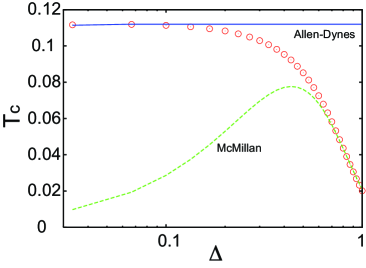
Figure 8: (Color online) Superconducting transition temperature $T_{\rm c}$ vs the phonon energy $\Delta$ for the harmonic case $b=c_{1}=c_{2}=0$. The dashed line corresponds to $T^{M}_{\rm c}$ given by Eq. (27) and the solid line represents $T_{\rm c}^{AD}$ given by Eq. (31)

III.3 Superconducting transition temperature in anharmonic systems

Now, we discuss the effects of anharmonicity of phonon dynamics on $T_{\rm c}$. Figure 9 shows the dependence of $T_{\rm c}$ on the third-order anharmonic term $b$ of the ion potential, Eq. (4) for $c_{2}=0$, $0.01$, and $0.03$, at fixed $c_{1}=0.04$. All the three cases exhibit a pronounced peak around the crossover value $b=b^{*}$ as discussed in Sec. II for each $c_{2}$, and $T_{\rm c}$’s are strongly suppressed in the quantum tunneling states, i.e., for large $b>b^{*}$. The solid lines in the figure represent the McMillan’s formula $T^{M}_{\rm c}$ [Eq. (27)]. The agreement with the McMillan’s formula indicates that $T_{\rm c}$ is qualitatively given by the conventional theory of strong coupling superconductivity. Note that $\lambda$ and $\omega_{\rm log}$ vary with the temperature in the presence of anharmonicity and $T_{\rm c}^{M}$ are calculated by using these values evaluated at $T=T_{\rm c}$. For $b\lower 3.01385pt\hbox{$\ \overset{>}{\sim}\ $}b^{*}$, however, the discrepancy becomes large as shown in the inset of Fig. 9, and the effects of anharmonicity and the nature of the extreme strong coupling regime appear, which will be discussed later in Sec. III.5.

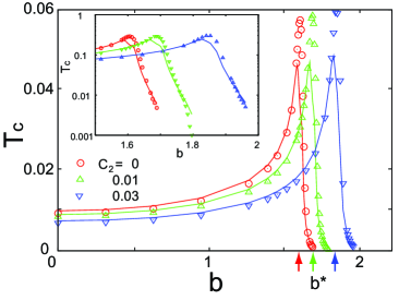
Figure 9: (Color online) $T_{\rm c}$ vs $b$ for $c_{1}=0.04$ and $c_{2}=$0, 0.01, and 0.03. The solid lines show $T_{\rm c}$’s of McMillan’s formula (27). $b^{*}$’s for each of $c_{2}$ are indicated by arrows. Inset: zoom up in the large $b$ part.

III.4 Competition between the energy scale and coupling constant

In Sec. III.4, we discuss the origin of the peak structure based on the McMillan formula.McMillan

The McMillan’s formula is expressed with the two parameters, $\lambda$ and $\omega_{\rm log}$, as shown in Eq. (27). In Fig. 10, we show the $b$ dependence of $\lambda$ and $\omega_{\rm log}$ calculated at $T_{\rm c}$ together with $\Delta$. It is noticeable that $\lambda$ shows a steep increase above $b^{*}$ and $\omega_{\rm log}$ is almost the same as $\Delta$ for $b\lower 3.01385pt\hbox{$\ \overset{<}{\sim}\ $}b^{*}$. From these facts, one can easily understand that $T_{\rm c}$ calculated by Eq. (27) decreases in the quantum tunneling states. The peak structure in $T_{\rm c}$ in Fig. 9 is a result of the competition between the suppression of $\omega_{\rm log}(\Delta)$ and the enhancement of $\lambda$. Thus, the peak structure is realized at $b\simeq b^{*}$, where $\lambda$ is large enough and simultaneously $\omega_{\rm log}$ is not vanishingly small.

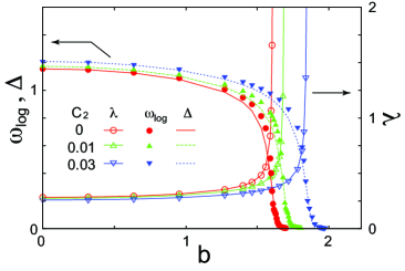
Figure 10: (Color online) $\lambda$, $\omega_{\rm log}$, and $\Delta$ vs $b$ for $c_{2}=0$, $0.01$, and $0.03$. The open symbols represent $\lambda$ and the filled symbols with a solid line represent $\omega_{\rm log}$. Lines without symbols represent $\Delta$. $\lambda$ and $\omega_{\rm log}$ are calculated at $T=T_{\rm c}$.

III.5 Strong coupling limit

In an extreme strong coupling regime $\lambda\gg 1$, Allen and Dynes showed that $T_{\rm c}$ is approximately given by Eq. (31) rather than the McMillan’s formula (27).AllenDynes When Eq. (31) is applied to our local phonon problem, we need care about the quantity $\lambda\langle\omega^{2}\rangle$. As pointed out by Hardy and Flocken,Hardy this quantity is related to the f-sum rule and this implies $T_{\rm c}$ is universal in any potential and depends only on the mass of the ion and $\alpha^{2}$ as shown in Fig. 8. However, this is not true in our anharmonic phonon system. From numerical calculations, instead of $\langle\omega^{2}\rangle$, we find that $T_{\rm c}$ for $b\gg b^{*}$ is approximately given by

$$T_{\rm c}=0.18\Delta\sqrt{\lambda}.$$ (32)

We note that the origin of large $\lambda$ for $b>b^{*}$ is the strong suppression of $\Delta$ for $b>b^{*}$ and other high-energy states do not play an important role. Thus, $\sqrt{\langle\omega^{2}\rangle}$ overestimate the energy scale of $T_{\rm c}$. These facts support the use of $\Delta$ instead of the averaged frequency $\sqrt{\langle\omega^{2}\rangle}$.

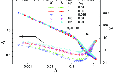
Figure 11: (Color online) $\lambda$, $\Delta^{\prime}$ vs $\Delta$ for $c_{2}=0.01$ and five sets of $\omega_{0}$ and $c_{1}$. The open (filled) symbols represent $\Delta^{\prime}$ ($\lambda$). $\Delta$ is controlled by varying $b$.

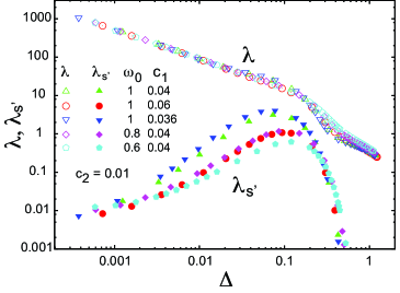
Figure 12: (Color online) $\lambda$ and $\lambda_{s^{\prime}}$ vs $\Delta$ for $c_{2}=0.01$ and five sets of $\omega_{0}$ and $c_{1}$. The open (filled) symbols represent $\lambda$ ($\lambda_{s^{\prime}}$).

III.6 Additional channel of attractive interactions

As we noted before, there is a crossover at $b=b^{*}$ to the quantum tunneling states and this means there are five states at low-energy region of the spectra as shown in Fig. 1. In the harmonic case, $\lambda$ is basically determined by the matrix element $\langle n|x|0\rangle$ between the ground state $|0\rangle$ and the threefold-degenerate first excited states, and the corresponding excitation energy $\Delta$. Since four low-energy excited states are nearly degenerate with the ground state around $b=b^{*}$, the singlet excited state $|s^{\prime}\rangle$ also has a noticeable matrix element $\langle n|x|s^{\prime}\rangle$. This provides another channel of attractive interaction and contributes to $T_{\rm c}$. It is important to note that this additional contribution never appears in the one-dimensional model and is a direct consequence of the crossover of the ground state at $b=b^{*}$.

In Fig. 11, we show $\lambda$ and the energy difference between $s^{\prime}$ state and the $p$-wave like first excited states: $\Delta^{\prime}=E_{s^{\prime}}-E_{p}$. They are calculated with varying $b$, and plotted as a function of the energy difference $\Delta$ between the first excited state and the ground state. $\lambda$ increases roughly as $\sim\Delta^{-3/4}$ for small $\Delta$. $\Delta^{\prime}$ shows minimum around $\Delta\sim 0.2$ and this reflects the anti-crossing in the energy spectra. Corresponding to this, the coupling constant $\lambda_{s^{\prime}}$ related to $s^{\prime}$ state shows a maximum around $\Delta\sim 0.1$ as shown in Fig. 12. Here, we define $\lambda_{s^{\prime}}$ as

$$\lambda_{s^{\prime}}=2\alpha^{2}\sum_{n=p}(w_{n}-w_{\rm s^{\prime}})|\langle n|x|{\rm s^{\prime}}\rangle|^{2}/(E_{\rm s^{\prime}}-E_{n}),$$ (33)

where the $n$ summation is taken over the three first excited states. Note that the smaller $\Delta^{\prime}$ is, the larger $\lambda_{s^{\prime}}$ is obtained. Depending on the magnitude of $\lambda_{s^{\prime}}$, total $\lambda$ has a small bump around the $\Delta\sim 0.1$ as a function of $\Delta$. This observation clearly shows that there is a new channel of interaction via the excitations between the first excited states and the $s^{\prime}$ state.

III.7 Deviations from Allen-Dynes formula near $b=b^{*}$

As we discussed in Sec. III.6, the enhancement of $\lambda_{s^{\prime}}$ influences the total $\lambda$ and also affects $T_{\rm c}$ itself. In Sec. III.7, we derive a formula which includes the contribution of $\lambda_{s^{\prime}}$. In order to take into account this contribution in Eq. (32), we assume the DOS given by

$$F(\omega)=\frac{\omega}{2}\Big{[}\lambda_{p}\delta(\omega-\Delta)+\lambda_{s^{\prime}}\delta(\omega-\Delta^{\prime})\Big{]}.$$ (34)

Since the enhancement of $\lambda_{s^{\prime}}$ takes place in a finite but extremely strong coupling regime, the total $\lambda$ is large and we follow the discussion by Allen and Dynes to estimate the lower bound of $T_{\rm c}$, by assuming a trial gap function $\Delta_{\rm SC}(i\omega_{n})=\Delta_{\rm SC}^{0}\delta_{|\omega_{n}|,\pi T}$.AllenDynes Using the form (34), we obtain the lower bound of $T_{\rm c}$ as

$$8\pi^{2}T_{\rm c}^{2} = \lambda_{p}\Delta^{2}+(\lambda_{s^{\prime}}-1){\Delta^{\prime}}^{2}$$

$$+ \sqrt{[\lambda_{p}\Delta^{2}+(\lambda_{s^{\prime}}-1){\Delta^{\prime}}^{2}]^{2}+4(\lambda_{p}+\lambda_{s^{\prime}})\Delta^{2}{\Delta^{\prime}}^{2}},$$

In the limit of $\lambda_{s^{\prime}}\to 0$ Eq. (LABEL:solution0) reduces to Eq. (32): $T_{\rm c}=\Delta\sqrt{\lambda_{p}}/(2\pi)$. Although the more sophisticated gap function can give the almost correct coefficient $0.18$ instead of $(2\pi)^{-1}$,AllenDynes it is enough to consider the simplest trial gap function in order to examine the contributions of the $s^{\prime}$ state to $T_{\rm c}$. In Eq. (LABEL:solution0), we assume $\lambda_{p}(\gg 1)$ corresponds to the coupling constant originating from the transition between the ground state and $p$-wave like states (first excited states) and $\lambda_{s^{\prime}}\ll\lambda_{p}$ is the part from $s^{\prime}$ state [Eq. (33)]. Since $\lambda_{p}\gg\lambda_{s^{\prime}}$, we can obtain a simpler approximate form of Eq. (LABEL:solution0). This is obtained by simply replacing $\lambda$ in Eq. (32) by $\lambda_{\rm eff}$,

$$\lambda_{\rm eff}=\lambda_{p}\Bigg{[}1+\frac{\lambda_{s^{\prime}}}{1+2\lambda_{p}\Big{(}\frac{\Delta}{\Delta^{\prime}}\Big{)}^{2}}\Bigg{]}.$$ (36)

Figure 13 shows the $\lambda$ dependence of $T_{\rm c}/\Delta$ for two typical sets of parameters in log-log scale. As shown with the dashed line, the Allen-Dynes formula shows a straight line. For small $\lambda$, the calculated values agree with the McMillan’s formula, while for extremely large $\lambda$ they approach the line of the Allen-Dynes formula. For the intermediate $\lambda>1$, however, the results show a bending and this bending is larger in Fig. 13(b) than in Fig. 13(a). Our two-channel formula (LABEL:solution0) can describe the bending as indicated by the solid line. Although the lower bound of $T_{\rm c}$, Eq. (LABEL:solution0) is not in very good agreement with the calculated $T_{\rm c}$, it captures the overall behavior of $T_{\rm c}$ for $\lambda>1$. It is also noted that, although the McMillan’s formula (27) shows an increase in $T_{\rm c}/\Delta$ for large $\lambda$, the increase is too steep. The present two-component analysis confirms the existence of the additional channel of the interaction near the crossover point in this system.

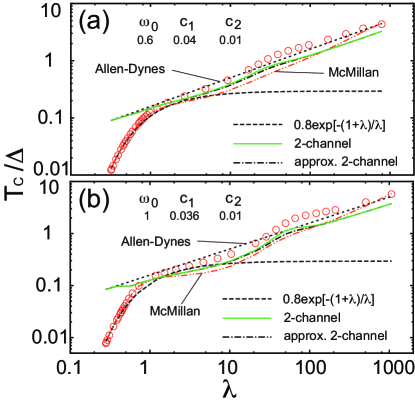
Figure 13: (Color online) Various $T_{\rm c}$ formulas (27), (31), (LABEL:solution0), and (36) vs $\lambda$. Formula (27) with $\omega_{\rm log}$ replaced by $\Delta$ is also plotted for comparison. (a) $\omega_{0}=0.6$, $c_{1}=0.04$, and $c_{2}=0.01$. (b) $\omega_{0}=1$, $c_{1}=0.036$, and $c_{2}=0.01$.

IV Discussions

Let us now discuss the implications of our calculations to compare with characteristic properties experimentally observed in $\beta$-pyrochlore compounds. One point is the chemical trends among the three member compounds, and we discuss why the potassium compound has the highest $T_{\rm c}$ of superconductivity. Another point is about the question why the superconducting phase is not so much affected by the isomorphic structure transition at $T_{p}$ in the phase diagram. We will also propose a possible change in the K-oscillation profile at $T_{p}$ and the effects of the transition on superconductivity.

IV.1 Chemical trends in $\beta$-pyrochlore compounds

Among the three $\beta$-pyrochlore compounds $A$Os₂O₆ ($A$=K, Rb or Cs), the K compound has the highest $T_{\rm c}^{\mathrm{K}}$=9.6 K of superconductivity and the strongest anharmonicity in the $A$-cation oscillation dynamics as observed in the neutron-scattering experiments: the Debye-Waller factor of K ion is much smaller than of Rb and Cs compoundsNeutronSasai and the softening of the low-energy phonon peak is also the strongest in KOs₂O₆.Mukta The Rb compound has the next strongest anharmonicity and the second highest $T_{\rm c}^{\mathrm{Rb}}$=6.3 K, while the Cs compound has the weakest anharmonicity and the lowest $T_{\rm c}^{\mathrm{Cs}}$=3.3 K. The ratio of $T_{\rm c}$ is approximately 3:2:1. Thus, the anharmonicity in the ion dynamics and the value of $T_{\rm c}$ are related. Let us examine this point in our results and also check if one can explain, at least qualitatively, the trends of other important quantities, electron mass enhancement and phonon energy.

A crucial difference among the three compounds is the size of $A$-cation; the K ion has the smallest size, followed by Rb, and Cs is the biggest ion. Since the size of the surrounding Os₁₂O₁₈ cage essentially does not change, the K ion has the largest space inside the cage,Yamaura leading to strongly anharmonic oscillations. This reflects in different shapes of the $A$-cation potential, as shown in the calculation by Kuneš, et al.,BandCal although the point-group symmetry is common.

In our theory, the compound-dependent potential shapes are modeled by adjusting parameters in the potential, Eq. (2) or (4). In the following, we will show that $T_{\rm c}$ values and the ion dynamics in the three compounds are naturally explained by appropriate choice of potential parameters. Throughout Sec. IV.1, we will use some parameters explicitly shown with physical dimensions if necessary.

Let us first consider the trend of the value $b/b^{*}$ among the three compounds, recalling the anharmonicity appearing in the Debye-Waller factor and the phonon energy observed in the neutron experiments. NeutronSasai ; Mukta As shown in Fig. 4, the anharmonicity grows with $b/b^{*}$. This implies that the $b/b^{*}$ value is the smallest for Cs, then for Rb, and the largest for K. Note that the largest ratio is still smaller than or at most equal to the crossover value $b/b^{*}=1$, since the observed K-cation density profile does not change its peak position from the equilibrium position.Yamaura ; newSasai

Secondly, we consider the trend of the second-order potential parameter $\omega_{0}$. Figure 14 shows the $b$ dependence of $T_{\rm c}$ for several values of $\omega_{0}$. The first-principle calculation of the ion potential clearly shows that $\omega_{0}$ is very small for K while larger for Rb and the largest for Cs.NoteBandCalc This trend is consistent with the fact that the K compound has the strongest anharmonicity and the highest $T_{\rm c}$ as far as $b<b^{*}$, as shown in Fig. 14. It is also important to note that the peak position $\sim b^{*}$ becomes smaller as $\omega_{0}$ decreases.

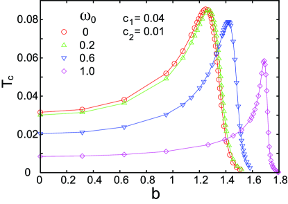
Figure 14: (Color online) $T_{\rm c}$ vs $b$ for five values of $\omega_{0}$ fixing $c_{1}=0.04$ and $c_{2}=0.01$.

By keeping these variations in $b/b^{*}$ and $\omega_{0}$ in mind, let us discuss our results of $\Delta$, $\lambda$ at $T=T_{\rm c}$ and $T_{\rm c}$ itself for each of the three compounds. In order to make discussion simple, we assume the electron phonon coupling and the electron density of states are the same for the three compounds and $\alpha^{2}=1897$ K/Ų. The atomic mass of each $A$-cation is $M_{\rm K}=71748m_{e}$, $M_{\rm Rb}=156839m_{e}$, and $M_{\rm Cs}=243890m_{e}$, respectively. We have adjusted potential parameters, Eq. (2), for each compound to reproduce the phonon energy and the effective ion oscillation variance $\langle x^{2}\rangle_{\rm exp}$ determined from the Debye-Waller factor.NeutronSasai ; Mukta ; Galati As shown in Sec. II.4, $W_{\bf d}({\bf Q})$ generally contains the contribution of the third-order fluctuations $\langle xyz\rangle$ in addition to $\langle x^{2}\rangle$. However, since the experimental data is the ${\bf Q}$-averaged value of $\overline{W_{{\bf d}}({\bf Q})/|{\bf Q}|^{2}}$, it is sufficient to consider the second-order fluctuations $\langle W_{{\bf d}}({\bf Q})/|{\bf Q}|^{2}\rangle=\frac{1}{6}\langle|{\bf u_{d}}|^{2}\rangle=\frac{1}{2}\langle x^{2}\rangle$. Since our potential, Eq. (2) or (4), includes four parameters, we fix $B=9324$ K/ų and $C_{1}=4C_{2}=3332$ K/Å⁴ for simplicity and vary $\Omega_{0}$. It is noted that $\Omega_{0}$ is expected to become smaller as the size of the alkali cation decreases, and, for fixed $B$, $b/b^{*}$ becomes smaller as $\Omega_{0}$ increases.

Table 1 shows the list of the basic quantities, $\Delta$, $\lambda$, and $T_{\rm c}$ for the three compounds. Let us first discuss $T_{\rm c}$. It is quite sure that one needs also to include a high-energy phonon, which plays a role to increase the $T_{\rm c}$ by about 3-5 K for all the three compounds, to obtain $T_{\rm c}$ consistent with the experimental results. $T_{\rm c}^{(2)}$ is one calculated with including an additional phonon with energy $\hbar\Omega_{h}=260$ K. We have set the corresponding dimensionless coupling constant $\lambda_{h}=0.256$ in the calculations. The results of $T_{\rm c}^{(2)}$ are quantitatively consistent with the experimental values $T_{\rm c}^{\rm K}=9.6$ K, $T_{\rm c}^{\rm Rb}=6.3$ K, and $T_{\rm c}^{\rm Cs}=3.3$ K. Here, we can reproduce the experimental values of $T_{\rm c}$ by assuming the same $\alpha^{2}$, $\lambda_{h}$ and $\Omega_{h}$ for all the three compounds and we conclude that the origin of the difference in $T_{\rm c}$ for the three $\beta$-pyrochlore compounds is due to the difference mainly in the anharmonicity of the alkali cation oscillations.InThisPoint

Now, let us discuss the electron effective mass. In our theory, the electron mass enhancement factor is related to $\lambda_{\rm tot}$ as $1/z_{\rm tot}=1+\lambda_{\rm tot}$. $\lambda$’s obtained from experiments and previous theoretical studies are $\lambda^{\rm K}=$1.6-2.4, SummaryHiroi ; BattloggSC ; Nagao ; Chang for K, $\lambda^{\rm Rb}=$1.0-1.3, Nagao ; Manalo for Rb and $\lambda^{\rm Cs}=0.78$,Nagao for Cs, respectively. Our estimation of $\lambda_{\rm tot}=\lambda+\lambda_{h}=\lambda+0.256$ with $\lambda$ in Table 1 is qualitatively consistent with these values, although we have not fit $T_{\rm c}$ for each compound. The experimental values of specific-heat coefficient $\gamma$ is $\gamma_{\rm K}=70$, $\gamma_{\rm Rb}=45$, and $\gamma_{\rm Cs}=41$ mJ/mol K² while the band calculations predicted $\gamma_{0}\sim 10$ mJ/mol K² for all the three compounds.Nagao ; bandmass Thus, the experimental mass enhancement factor $\gamma_{\rm K}/\gamma_{0}$ in KOs₂O₆ is 1.5-1.7 times larger than in RbOs₂O₆ and CsOs₂O₆ele-ele . In our calculation, $z_{\rm tot}^{\rm Rb}/z_{\rm tot}^{\rm K}\simeq 1.71$ and $z_{\rm tot}^{\rm Cs}/z_{\rm tot}^{\rm K}\simeq 1.98$, which are semi-quantitatively consistent with the experimental values. From our results, the enhanced mass enhancement in KOs₂O₆ is attributed to the proximity to the crossover to the quantum tunneling state and also the large oscillation amplitude, which effectively enhances the electron-phonon coupling.

In order to obtain the correct value of the mass enhancement ($\sim 7$ for KOs₂O₆ and $\sim 4$ for the other two), we should also take into account the electron-electron interactions, but this is beyond the scope of the present study and we leave it for a future problem. Nevertheless, it is important to note that $\lambda$ is significantly enhanced near $b=b^{*}$ by anharmonic oscillations and that this is the central reason why the mass enhancement in KOs₂O₆ is much larger than in Rb and Cs compounds.

As for the phonon frequency $\Delta$, optical modes related to the $A$-cation oscillations are observed at energy around 5-7 meV at room temperature in the inelastic neutron scatteringNeutronSasai ; Mukta and their energies show strong softening as the temperature decreases. This corresponds to our results shown in Fig. 7. For KOs₂O₆, the phonon energy at $T=1.5$ K is about 3.1 meV, which is quite small compared with the value of 5.5 meV at $T=300$ K.Mukta Furthermore, the low-energy phonon peaks in KOs₂O₆ are rather broad compared with Rb and Cs compounds,Mukta which suggests the proximity to the crossover point. The specific-heat experimentSummaryHiroi and the photo-emission spectroscopy dataPES also support these results.

In our calculation for KOs₂O₆ with parameters in Table 1, the peak position in the phonon spectrum is about 70 K $\simeq$ 6 meV at $T=300$ K and this shifts to $\Delta=38.5$ K as $T$ decreases. This means the potential parameters in Table 1 can reproduce not only $T_{\rm c}$ and $\Delta$ but also the temperature dependence of the spectra.

As for the chemical trends, we have calculated superconducting transition temperature for the three $\beta$-pyrochlore compounds adjusting parameters in the potential, Eq. (2), and we can reproduce the phonon energy and amplitude related to the average Debye-Waller factor. We have obtained quantitatively consistent values of $T_{\rm c}$ with the experimental ones, using the same electron-phonon coupling, the electron DOS and also the same additional high-energy phonon for all the three compounds.

Table 1: Local potential parameters and $\langle x^{2}\rangle$ at $T\!=\!0$, $\lambda$ at $T=T_{\rm c}$, $\Delta$, $T_{\rm c}$, and $T_{\rm c}^{(2)}$ for the three $\beta$-pyrochlore compounds. The other parameters are $B=9324\ {\rm K/\AA}^{3}$, $C_{2}=C_{1}/4=3332$ K/Å⁴, and $\alpha^{2}=1897\ {\rm K/\AA}^{2}$.

	$\hbar\Omega_{0}({\rm K})$	$b/b^{*}$	$\langle x^{2}\rangle(T=0)$(Å2)	$\lambda$	$\Delta$(K)	$T_{\rm c}$(K)	$T_{\rm c}^{(2)}$(K)
K	26.4	0.58	0.0152	1.47	38.5	6.45	10.5
Rb	54.6	0.28	0.0050	0.34	56.2	0.82	5.74
Cs	74.8	0.11	0.0024	0.12	75.2	$<$0.03	3.37

IV.2 Changes at $T_{p}$

As mentioned in Sec. I, KOs₂O₆ exhibits an isomorphic first-order transition at $T_{p}=7.5$ K.SummaryHiroi ; Hasegawa ; newSasai In Sec. IV.2, let us investigate the effects of this transition on the phonon dynamics, using a set of constraints offered by the experimental results. We also discuss its effects on superconductivity.

Electric resistivity shows a concave temperature dependence at high temperatures, and this is attributed to the strong coupling to phonons with strong anharmonicity.SummaryHiroi ; DahmUeda At the magnetic field $H=14$ T, the resistivity is suddenly suppressed by 25 % at $T_{p}$, and shows a different $T$-dependence proportional to $T^{2}$ at $T_{\rm c}<T<T_{p}$.SummaryHiroi This indicates that the electron-phonon scattering processes are reduced significantly at $T_{p}$SummaryHiroi . This is also consistent with the reduction in the specific-heat jump at $T_{\rm c}$ in magnetic fields above 8 T.SummaryHiroi

In the magnetic field-temperature phase diagram, $T_{p}$ remains essentially insensitive to magnetic field $H$ as shown in Fig. 15. The upper critical magnetic field $H_{c2}$ is suppressed below $T_{p}$, but extrapolating to the region above $T_{p}$, it seems that it also vanishes at the position very close to $T_{\rm c}(H=0)$.

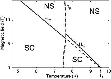
Figure 15: Schematic temperature-magnetic field phase diagram taken from Ref. 3. The solid and dotted lines represent $H_{c2}$ and $T_{p}$, respectively. The dashed line indicates the extrapolation of low-$T$ $H_{c2}$ to the higher-temperature region.

This fact cannot be explained if the characteristic energy scale, $\omega_{\rm log}$ or $\Delta$ is common across $T_{p}$: the extrapolated $H_{c2}$ line should vanish below $T_{\rm c}(H=0)$ since $\lambda$ is reduced below $T_{p}$ as discussed above. Therefore, the above fact implies the enhancement of the characteristic energy scale $\Delta$ or $\omega_{\rm log}$ below $T_{p}$. Indeed, Chang, et al.,Chang assumed a slightly increased Einstein energy to fit the specific heat data and our previous study also predicted the increase in the oscillation energy.Hat

Let us discuss the changes in $\lambda$, $\Delta$, $|\langle x^{2}\rangle|$, and $|\langle xyz\rangle|$ at $T_{p}$ based on our results, modeling the isomorphic transition by a sudden change in the two potential parameters, $\omega_{0}$ and $b$. This change corresponds to the variation in the mean field part of inter-site ion interactions, which was discussed in Ref. 34 and also changes in the oxygen positions and the lattice constant.newSasai Two parameters are chosen under the constraints (i) two different parameter sets above and below $T_{p}$ lead to the same $T_{\rm c}$, and (ii) $\lambda$ is smaller below $T_{p}$, both of which are the experimental constraints, and we also assume (iii) no significant change in the electron band structure across the transition and thus $\alpha^{2}$ is also unchanged, and (iv) $b<b^{*}$ for both below and above $T_{p}$ implied by the result of the electron-density profile obtained by the x-ray and the neutron experiments Yamaura ; newSasai as discussed before. In the following, we discuss the change across $T_{p}$ based on these constraints.

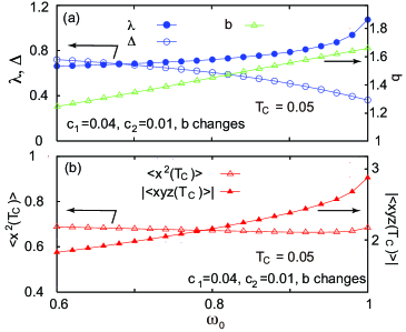
Figure 16: (Color online) $\omega_{0}$ dependence of characteristic quantities, when $T_{\rm c}$ is fixed to 0.05 by tuning $b$. (a) $\lambda$, $\Delta$, and $b$. (b) The second and third-order moments of ion oscillation $\langle x^{2}\rangle$, and $|\langle xyz\rangle|$. $c_{1}=0.04$ and $c_{2}=0.01$.

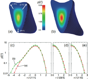
Figure 17: (Color online) Ion density isosurface for $\rho({\bf r})=0.05$ and the density map on the section with (110) plane at $T=0.002$. (a) $\omega_{0}=0.8$, $b=1.44$ and (b) $\omega_{0}=1$, $b=1.66$. (c) $\rho({\bf r})$ along [111] direction corresponding to (a) and (b), (d) along [001] and (e) along [110] direction. $\rho(-|{\bf r}|)$’s in (d) and (e) are not shown since $\rho({\bf r})=\rho(-{\bf r})$ along these directions.

In Fig. 16, characteristic quantities are shown for fixed $c_{1}$ and $c_{2}$ with varying $\omega_{0}$ and simultaneously $b$ such that those give the same $T_{\rm c}=0.05$. Since $b<b^{*}$ which is the assumption (iv), $T_{\rm c}$ is well approximated by the McMillan formula (27), in which $T_{\rm c}$ is determined by the two factors $\omega_{\rm log}\simeq\Delta$ and $\lambda$.

Firstly, it is noted that $\lambda$ increases as $\omega_{0}$ increases. One might expect a suppression of $\lambda$ as $\omega_{0}$ increases, but the key point is that we simultaneously tune $b$ to fix $T_{\rm c}$ unchanged and this means larger $b$ is necessary at larger $\omega_{0}$. This increase in $b$ overcomes the competing effect of the increase in $\omega_{0}$, and finally $\lambda$ increases. Secondly, the energy of the first excited state $\Delta$ increases as $\omega_{0}$ decreases. This is naturally understood by noting that $\Delta$ becomes large for smaller $b$. Thus, from the constraint (ii) the above results imply that the phonon energy is enhanced below $T_{p}$ and, indeed, this is consistent with the previous theoretical studies.Chang ; Hat

Most interestingly, the second- and third-order fluctuations $\langle x^{2}\rangle$ and $|\langle xyz\rangle|$ change oppositely as shown in Fig. 16(b). As $\omega_{0}$ decreases, $\langle x^{2}\rangle$ increases for the most of the $\omega_{0}$ range, while $|\langle xyz\rangle|$ decreases monotonically. This is because small $\omega_{0}$ corresponds to small $b$ as explained above. These results indicate that $\langle x^{2}\rangle$ is slightly enhanced below $T_{p}$ while $|\langle xyz\rangle|$ is suppressed.

In order to illustrate these anisotropic fluctuations, the density isosurface for $\rho({\bf r})=0.05$ and the density (color) map are shown for two different parameters at $T=0.002$ in Fig. 17: for (a) and (b), $\omega_{0}=0.8$ and $1.0$, and $b=1.44$ and $1.66$, respectively, and these two sets give the same $T_{\rm c}=0.045$, and we choose the two parameter sets to emphasize the change in the oscillation profile. As expected from the values of $b$, the case (a) has the smaller $\lambda=0.647$ and the larger $\Delta=0.662$, while $\lambda=0.782$ and $\Delta=0.429$ for the case (b).

One can see that the density isosurface shows more anisotropic character in the case (b), where the “spikes” sticking out along four [111] directions are sharper than those in the case (a). This aspect reflects in the values of $\langle x^{2}\rangle$ and $\langle xyz\rangle$. Indeed, $\langle x^{2}\rangle$ at $T=T_{\rm c}$ is larger $\langle x^{2}\rangle=0.645$ in (a) than $0.626$ in (b), while $|\langle xyz\rangle|$ at $T=T_{\rm c}$ is smaller $|\langle xyz\rangle|=1.93$ in (a) than $2.35$ in (b). Figures 17(c)-17(e) show $\rho({\bf r})$ along [111], [001], and [110] directions, respectively, for the same two data. It is clearly seen that $|\langle xyz\rangle|$ in (b) is larger than that in (a) as shown in (c), and $\langle x^{2}\rangle$ in (a) is larger than in (b) as shown in (d) and (e).

These changes in the anisotropy of density distribution is a characteristic nature of the first-order isomorphic transition at $T_{p}$. This transition is isomorphic, consistent with the experiments,SummaryHiroi ; Hasegawa because the amplitude of anisotropy changes but it does not break the point group, translational, and any other symmetries. Our results suggest that $\langle x^{2}\rangle$ is slightly enhanced while $|\langle xyz\rangle|$ is suppressed below $T_{p}$ in KOs₂O₆. Recent high-resolution neutron-scattering experiment shows the increase in $\langle x^{2}\rangle$ across $T_{p}$ as $T$ decreases,newSasai which is consistent with our result.

Furthermore, although it is naively expected that an increase in $\langle x^{2}\rangle$ corresponds to the enhancement of $\lambda$, this does not necessarily hold in this system, since the value of $\lambda$ is sensitive to the value of $b$, especially near the crossover point $b^{*}$. Our results show that the value of $|\langle xyz\rangle|$ plays more important role for the enhancement of $\lambda$ than $\langle x^{2}\rangle$. In order to detect this change in the density distribution across $T_{p}$, it is important to perform detailed neutron-scattering experiments and to analyze the results with taking into account the third-order term in Debye-Waller factor as discussed in Sec. II.4. It is worthwhile to examine the ${\bf Q}$ dependence of the Debye-Waller factor to extract the anisotropy of the oscillations, since ${\bf Q}$-averaged Debye-Waller factor hinders the anisotropy and anharmonicity.

Finally, we comment on the possibility of re-entrant superconducting transition. Experimentally, Hiroi et al.,SummaryHiroi observed a re-entrant superconducting transition around $H=7$ T as shown in Fig. 15. This can be understood from $H_{c2}(T=0)$ in the strong coupling theory of superconductivity:

$$H_{c2}(T=0)\propto T_{\rm c}^{2}(1+\lambda)^{2}(1+1.44\frac{T_{\rm c}}{\omega_{\rm log}}+\cdots),$$ (37)

for the clean limit.Carbotte In our analysis, the $\lambda$ decreases and $\omega_{\rm log}$ increases below $T_{p}$, while the $T_{\rm c}$ is approximately the same for the potential parameters above and below $T_{p}$. Thus, $H_{c2}(T=0)$ for the low-$T$ parameter set is smaller than that for the high-$T$ set. Therefore, we expect a $H_{c2}(T)$ curve similar to that shown in Fig. 15. This result does not change when we use the formula for the dirty limit.Carbotte

V Summary

We have investigated in the present paper anharmonic phonons and strong coupling superconductivity in $\beta$-pyrochlore compounds, $A$Os₂O₆ ($A$=K, Rb, or Cs).

First, we have solved the Schrödinger equation of the three-dimensional anharmonic phonon in tetrahedral symmetry. The main issue is the importance of the third-order anharmonicity $bxyz$ in the ion potential allowed for this symmetry. We have determined the energy spectrum of the anharmonic phonon as a function of the third-order anharmonicity $b$. We have found that there exists a crossover of the ground state to the quantum tunneling state for $b>b^{*}$. We have pointed out non-monotonic temperature dependence of ion density profile near the crossover point $b^{*}$.

Secondly, we have calculated the transition temperature of superconductivity $T_{\rm c}$ mediated by these anharmonic phonons. We have found that the enhancement of $T_{\rm c}$ near $b=b^{*}$. Its $b$ dependence can be well fitted by the McMillan formula at $b\lower 3.01385pt\hbox{$\ \overset{<}{\sim}\ $}b^{*}$. For $b\lower 3.01385pt\hbox{$\ \overset{>}{\sim}\ $}b^{*}$ we have found that there exists an additional channel of pairing interaction, which turns out to originate from low-energy excited states appearing at $b\sim b^{*}$. We have analyzed its contribution and derived an approximated formula of $T_{\rm c}$ in the strong coupling limit.

We have also discussed the chemical trends of $T_{\rm c}$ in the $\beta$-pyrochlore family $A$Os₂O₆ ($A$=K, Rb, or Cs). The main difference among the three members are different values of $b/b^{*}$ and the second-order term in the ion potential $\omega_{0}$. By assuming the same electron-phonon coupling constant $\alpha^{2}$ and the same high-energy phonon for all the three compounds, the differences in $T_{\rm c}$ and the energy of the first excited phonon states $\Delta$ have been quantitatively explained only by the difference in the local anharmonic potential.

Finally, we have discussed the effect of the first-order transition observed in KOs₂O₆. The changes in the density distribution of K cation at the first-order transition have been discussed based on the experimental data obtained so far. Especially, we have found that $\langle x^{2}\rangle$ and $|\langle xyz\rangle|$ change differently across $T_{p}$. Our results suggest the increase in the first excited phonon energy $\Delta$ and the reduction in the dimensionless electron-phonon coupling constant $\lambda$ across $T_{p}$. While the latter is consistent with the experimental results, the former has not been observed and this is our prediction for the experiments. In order to detect the increase in $\Delta$, it is important to carry out the high-resolution inelastic neutron scattering experiments. We hope our results shed lights in $\beta$-pyrochlore compounds both on the strong coupling superconductivity and on the anharmonic oscillations observed.

- (1) Z. Hiroi, S. Yonezawa, and Y. Muraoka, J. Phys. Soc. Jpn. 73, 1651 (2004).
- (2) Z. Hiroi, S. Yonezawa, J. Yamaura, T. Muramatsu and Y. Muraoka, J. Phys. Soc. Jpn. 74, 1682 (2005).
- (3) Z. Hiroi, S. Yonezawa, Y. Nagao and J. Yamaura, Phys. Rev. B 76, 014523 (2007).
- (4) T. Hasegawa, Y. Takasu, N. Ogita, M. Udagawa, J. I. Yamaura, Y. Nagao, and Z. Hiroi, Phys. Rev. B 77, 064303 (2008).
- (5) T. Goto, Y. Nemoto, K. Sakai, T. Yamaguchi, M. Akatsu, T. Yanagisawa, H. Hazama, K. Onuki, H. Sugawara, and H. Sato, Phys. Rev. B 69, 180511(R) (2004).
- (6) K. Kaneko, N. Metoki, H. Kimura, Y. Noda, T. D. Matsuda, and M. Kohgi, J. Phys. Soc. Jpn. 78, 074710 (2009).
- (7) H. Kotegawa, H. Hidaka, T. C. Kobayashi, D. Kikuchi, H. Sugawara, and H. Sato, Phys. Rev. Lett. 99, 156408 (2007).
- (8) B. C. Sales, B. C. Chakoumakos, R. Jin, J. R. Thompson, and D. Mandrus, Phys. Rev. B 63, 245113 (2001).
- (9) I. Zerec, V. Keppens, M. A. McGuire, D. Mandrus, B. C. Sales, and P. Thalmeier, Phys. Rev. Lett. 92, 185502 (2004).
- (10) H. Matsumoto, T. Mori, K. Iwamoto, S. Goshima, S. Kushibiki, and N. Toyota, Phys. Rev. B 79, 214306 (2009).
- (11) Y. Kasahara, Y. Shimono, T. Shibauchi, Y. Matsuda, S. Yonezawa, Y. Muraoka, and Z. Hiroi, Phys. Rev. Lett. 96, 247004 (2006).
- (12) M. Yoshida, K. Arai, R. Kaido, M. Takigawa, S. Yonezawa, Y. Muraoka, and Z. Hiroi, Phys. Rev. Lett. 98, 197002 (2007).
- (13) Y. Nakai, K. Ishida, H. Sugawara, D. Kikuchi, and H. Sato, Phys. Rev. B 77, 041101(R) (2008).
- (14) Y. Nemoto, T. Yamaguchi, T. Horino, M. Akatsu, T. Yanagisawa, T. Goto, O. Suzuki, A. Dönni, and T. Komatsubara, Phys. Rev. B 68, 184109 (2003).
- (15) I. Ishii, T. Fujita, I. Mori, H. Sugawara, M. Yoshizawa, K. Takegahara, and T. Suzuki, J. Phys. Soc. Jpn. 78, 084601 (2009).
- (16) Y. Nakanishi and M. Yoshizawa (private communications).
- (17) M. Brühwiler, S. M. Kazakov, J. Karpinski, and B. Batlogg, Phys. Rev. B 73, 094518 (2006).
- (18) I. Bonalde, R. Ribeiro, W. Brämer-Escamilla, J. Yamaura, Y. Nagao, and Z. Hiroi, Phys. Rev. Lett. 98, 227003 (2007).
- (19) Y. Shimono, T. Shibauchi, Y. Kasahara, T. Kato, K. Hashimoto, Y. Matsuda, J. Yamaura, Y. Nagao, and Z. Hiroi, Phys. Rev. Lett. 98, 257004 (2007).
- (20) Y. Nagao, J. Yamaura, H. Ogusu, Y. Okamoto, and Z. Hiroi, J. Phys. Soc. Jpn. 78, 064702 (2009).
- (21) J. Chang, I. Eremin, P. Thalmeier, and P. Fulde, Phys. Rev. B 76, 220510(R) (2007).
- (22) J. Chang, I. Elemin, and P. Thalmeier, New J. Phys. 11, 055068 (2009).
- (23) T. Dahm and K. Ueda, Phys. Rev. Lett. 99, 187003 (2007).
- (24) A. Yamakage and Y. Kuramoto, J. Phys. Soc. Jpn. 78, 064602 (2009).
- (25) K. Sasai, K. Hirota, Y. Nagao, S. Yonezawa, and Z. Hiroi, J. Phys. Soc. Jpn. 76, 104603 (2007).
- (26) R. Galati, C. Simon, P. F. Henry, and M. T. Weller, Phys. Rev. B 77, 104523 (2008).
- (27) H. Mutka, M. M. Koza, M. R. Johnson, Z. Hiroi, J. I. Yamaura, and Y. Nagao, Phys. Rev. B 78, 104307 (2008).
- (28) N. M. Plakida, V. L. Aksenov, and S. L. Drechsler, Europhys. Lett. 4, 1309 (1987).
- (29) J. R. Hardy and J. W. Flocken, Phys. Rev. Lett. 60, 2191 (1988).
- (30) V. H. Crespi and M. L. Cohen, Phys. Rev. B. 48, 398 (1993).
- (31) G. D. Mahan and J. O. Sofo, Phys. Rev. B 47, 8050 (1993).
- (32) S. Manalo, H. Michor, G. Hilscher, M. Brühwiler and B. Batlogg, Phys. Rev. B 73, 224520 (2006).
- (33) J. Kuneš, T. Jeong, and W. E. Pickett, Phys. Rev. B 70, 174510 (2004); J. Kuneš and W. E. Pickett, Physica B 378-380, 898 (2006).
- (34) K. Hattori and H. Tsunetsugu, J. Phys. Soc. Jpn 78, 013603 (2009).
- (35) In those cases of , we keep the same energy unit of 44 K, instead of renormalization of energy. This simplifies our discussions about dependence in later sections.
- (36) S. W. Lovesey, Theory of Neutron Scattering from Condensed Matter (Clarendon Press, Oxford, 1984), Vol. 1..
- (37) K. Hattori and K. Miyake, J. Phys. Soc. Jpn. 76, 094603 (2007).
- (38) M. Takechi and K. Ueda, J. Phys. Soc. Jpn. 78, 024604 (2009).
- (39) G. M. Eliashberg, Zh. Eksp. Teor. Fiz. 38, 966 (1960) [Sov. Phys. JETP 11, 696 (1960)].
- (40) D. J. Scalapino, J. R. Schrieffer, and J. W. Wilkins, Phys. Rev. 148, 263 (1966).
- (41) A. A. Abrikosov, L. P. Gorkov, and I. Ye. Dzyaloshinskii, Quantum Field Theoretical Methods in Satistical Physics, 2nd ed. (Pergamon Press, Oxford, 1965).
- (42) G. Bergmann and D. Rainer, Z. Phys. 263, 59 (1973).
- (43) W. L. McMillan, Phys. Rev. 167, 331 (1968).
- (44) P. B. Allen and R. C. Dynes, Phys. Rev. B 12, 905 (1975).
- (45) When is expressed by the quantities with the dimension, , which is, indeed, dimensionless.
- (46) J. Yamaura, S. Yonezawa, Y. Muraoka, and Z. Hiroi, J. Solid State Chem. 179, 336 (2006).
- (47) K. Sasai, M. Kofu, R. M. Ibberson, K. Hirota, J. Yamaura, Z. Hiroi, and O. Yamamuro, J. Phys.: Condens. Matter 22, 015403 (2010).
- (48) The result in Ref. 33 suggests a slightly negative value of for KOs2O6. However, the first excited state then has an energy too small compared with the experimental estimate from the specific heat data (Ref. 3) and the neutron scattering (Refs. 25 and 27). Correspondingly, calculated is too large compared with the experimental results and its temperature dependence is qualitatively different from the experimental one (Refs. 25 and 26). In this paper, we consider the cases of for simplicity. We hope that more detailed information on the ion potential is provided by the neutron scattering experiments in the future.
- (49) In this point whether the additional phonon is acoustic or optical mode does not make an essential difference. To improve estimation of , we need the detailed information of each compound on the electron-phonon coupling , , , and other parameters.
- (50) Z. Hiroi, J. Yamaura, S. Yonezawa, and H. Harima, Physica C 460-462, 20 (2007).
- (51) Note that this value of the mass enhancement factor includes not only the contributions of electron-phonon interactions but also those of electron-electron interactions.
- (52) T. Shimojima, Y. Shibata, K. Ishizaka, T. Kiss, T. Tagoshi, A. Chainani, T. Yokoya, X.-Y. Wang, C. T. Chen, S. Watanabe, J. Yamaura, S. Yonezawa, Y. Muraoka, Z. Hiroi, T. Saitoh and S. Shin, Phys. Rev. Lett. 99, 117003 (2007).
- (53) J. P. Carbotte, Rev. Mod. Phys. 62, 1027 (1990).