Fixed points and limit cycles in the population dynamics of lysogenic viruses and their hosts

Abstract

Starting with stochastic rate equations for the fundamental interactions between microbes and their viruses, we derive a mean-field theory for the population dynamics of microbe-virus systems, including the effects of lysogeny. In the absence of lysogeny, our model is a generalization of that proposed phenomenologically by Weitz and Dushoff. In the presence of lysogeny, we analyze the possible states of the system, identifying a novel limit cycle, which we interpret physically. To test the robustness of our mean field calculations to demographic fluctuations, we have compared our results with stochastic simulations using the Gillespie algorithm. Finally, we estimate the range of parameters that delineate the various steady states of our model.

I Introduction

Microbes and their viruses are the most genetically diverse, abundant and widely distributed organisms across the planetMaranger and Bird (1995); Chibani-Chennoufi et al. (2004); Santelli et al. (2008); Ortmann and Suttle (2005). Microbes are major contributors to the global biogeochemical cycles and catalyze the reactions that have over evolutionary time brought the Earth’s surface to its present redox stateFalkowski et al. (2008). Similarly, viruses, especially in the oceans, manipulate marine communities through predation and horizontal gene transferSyvanen (1994); Ochman et al. (2000), recycle nutrients and thus drive the biological pump which leads inter alia to the sequestration of carbon in the deep oceanWilhelm and Suttle (1999); Suttle (2005); Weinbauer and Rassoulzadegan (2004); Sharma et al. (2006); Monson et al. (2006); Schimel et al. (2007); Suttle (2007); Danovaro et al. (2008); Bardgett et al. (2008); Rohwer and Thurber (2009).

It is being increasingly realized that the classical view of microbial viruses purely as predators is too limited. Many microbe-virus interactions are lysogenic, not lytic: upon infection, the viral genetic material is incorporated into the chromosome of the host, replicates with the host, and can be subsequently released, typically triggered by the stress response of the host to environmental changePaul (2008). As a result, viruses can transfer genes to and from bacteria, as well as being predators of them, so that the virosphere should properly be recognized as a massive gene reservoirSonea (1988); Sullivan et al. (2006); Goldenfeld and Woese (2007); Rohwer and Thurber (2009). Thus there is a coevolution of both communities, the effects of which are complex and far-reachingAnderson (1966, 1970); Filee et al. (2003); Weinbauer and Rassoulzadegan (2004); Sullivan et al. (2006); Lindell et al. (2007); Goldenfeld and Woese (2007); Rohwer and Thurber (2009), even including the manipulation of bacterial mutation ratesPal et al. (2007). This nontrivial interaction between microbes and viruses has not gone unnoticed, with wide interest among biologists, ecologists and geologistsHadas et al. (1997); Williamson et al. (2002); Brussow et al. (2004); Williamson and Paul (2004); Chibani-Chennoufi et al. (2004); Brussow (2005); Rosvall et al. (2006); Lindell et al. (2007); Paul (2008); Williamson et al. (2008); Weitz (2008).

These findings highlight the importance of considering ecosystem dynamics within an evolutionary context. Conversely, evolution needs to be properly understood as arising from a spatially-resolved ecological context, as was first recognized by Wallace over 150 years agoWallace (1855). That speciation, and adaptation in general, arises at a particular point in time and space has a number of deep consequences that have not yet been incorporated into current theory. First, it means that evolutionary dynamics proceeds by the propagation of fronts, resulting in a complex and dynamical pattern of speciation, adaptation and genome divergence that reflects its intrinsic dynamics and that of the heterogeneous and dynamical environmentIbrahim et al. (1996); Hallatschek and Nelson (2008); Hallatschek and Korolev (2009); Korolev et al. (2009). Second, as fronts expand, there are only a few pioneer organisms at the leading edge, and so demographic fluctuations are much larger than in the bulk. Such fluctuations profoundly influence the spatial structure of the populations, and during the last few years have been recognized to play a major role in population cyclesMcKane and Newman (2004) and even spatial pattern formationButler and Goldenfeld (2009). Third, the existence of horizontal gene transfer and genome rearrangement processes is strongly coupled to spatial distribution. For example, it is known that the probability of conjugation events is dependent on the local density, being essentially one/per generation in closely-packed biofilms, but an order of magnitude smaller in planktonic cultureBabic et al. (2008). Moreover, the mechanism of horizontal gene transfer is also dependent on the density, with viral-mediated transduction being the most relevant mechanism at low density. How these patterns of evolutionary dynamics and species distribution play out is essentially unexplored. However, there have recently been the first reports of observations of the coupling between evolutionary and ecological timescales. In one such system (a predator-prey system realized in rotifer-algae interactions), it has been demonstrated that rapid evolutionary dynamics is responsible for the unusual phase-lag characteristics of the observed population oscillationsYoshida et al. (2007). Thus, rapid evolution is not only a major force for adaptation, but can have marked ecological consequences too.

The complex interplay between evolution and the environment is nowhere more important than in early life, where the key questions concern how life emerged from abiotic geochemistry. Early life experienced demanding environments, whose closest modern day correspondence might be deep ocean hydrothermal vents or hot springs. It is known that there are high occurrence of lysogens in both environmentsOrtmann and Suttle (2005); Held and Whitaker (2009), suggesting that microbe-phage interactions might also be important in the early stages of life, with lysogens playing an important role as a reservoir of genes and perhaps even aiding in the stabilitization of early life populations through the limit cycle mechanism discussed in this paper.

Our goal in this paper is to lay a theoretical foundation for describing the interplay between ecology and evolution in the context of microbe-virus systems, as these are arguably amongst the most important and probably the simplest of the complex systems in biology. The questions that will ultimately interest us are the evolutionary pressures that tune genetic switches governing the lysis-lysogeny decision, as well as the factors that shape prophage induction in response to environmental stressLenski and May (1994); Koch (2007); Refardt and Rainey (2010). Such a foundation must begin with a proper account of the population dynamics itself, before coupling in detail to other levels of description involving genome dynamics, for example. Thus, we have chosen to focus in the present paper on the dynamics of microbe-virus systems, taking full account of both of the major viral pathways. In this paper, we are not specific about whether we are dealing with bacterial or archaeal viruses, but because most of the experiments to date are carried out on bacteria, we have tended to identify the microbes as bacteria and the viruses as phages, even though this is not required by the mathematics.

We are now ready to introduce the specific problem that we treat in this paper. Upon phage infection, there are two pathways awaiting the host bacteriumPtashne (2004). In the first pathway—lysis—the bacteriophage produces a large number of copies of itself utilizing the bacterium’s genetic material and molecular machinery. As a result, the bacterium ceases its metabolic function, and ruptures, releasing the newly-assembled bacteriophage inside. The other pathway is lysogeny. In this process, the intruder integrates its own DNA into the genome of the bacterium, enters a dormant stage and becomes a prophage. The infected bacterium is known as a lysogen—a relatively stable stateBæk et al. (2003), immune to superinfection from the same or related strains, and proceeding under normal replication life-cycles. The DNA of the bacteriophage is duplicated, along with that of the host during cell replication. The lysogenic state can be terminated by environmental stress such as starvation, pollution or ultraviolet irradiation, resulting in the process known as prophage induction: the exit of the prophage from the host genome, and subsequent lysis of the original bacterium and its bacterial descendants.

We now discuss briefly existing treatments of population dynamics in the context of microbe-virus systems. In 1977, Levin et al Levin et al. (1977) extended the celebrated Lotka-Volterra equations to model the dynamics between virulent phages and their victims, where only virulent phages are considered. A number of extensions have been proposed, extending the level of biological realism to include such features as the time delay arising between infection and lysis as well as the evolution of kinetic parametersWang et al. (1996); Bohannan and Lenski (1997); Beretta and Kuang (2001); Fort and Méndez (2002); Weitz et al. (2005). In 2007, Weitz and DushoffWeitz and Dushoff (2008) proposed another way to improve the classic predator-prey model. Their attempt was mainly based on the experimental observation that the ability of a bacteriophage to lyse hosts degrades when the bacteria approach their carrying capacityMiddelboe (2000); Brussaard (2004); Sillankorva et al. (2004). Adding a new term to account for the saturation of the infection of the bacteriophages, they obtained an interesting phase diagram in which the fate of the bacteria-phage community can depend on the initial conditions. However, the new term is put in by hand, based on intuition which needs detailed mathematical support. Furthermore, they focused on virulent phages and excluded the temperate ones that elicit lysogeny, now regarded as essential to the survival of microbial communities through fluctuating environmentsBrussow et al. (2004); Paul (2008); Williamson et al. (2008).

These works are based upon an ensemble-level description of the community, as in the classic work on predator-prey systemsSmith (1978). However, as is well-known Smith (1978), the simplest of these models fails to capture the intrinsic cyclical behavior of predator-prey populations despite apparently incorporating fully the basic interactions that should give rise to cycles. This paradox was resolved by the important work of McKane and NewmanMcKane and Newman (2004), who showed that cyclical effects could only be captured at the level of an individual-level model, and arose through the amplification of demographic noise. Their work showed how the conventional ensemble-level equations for predator-prey systems arose as the mean field limit of the appropriate statistical field theory, with the essential effects of demographic noise entering the analysis as one-loop corrections to mean field theory, in an inverse population size expansion. These effects can also be treated in a slightly more convenient formalism using path integralsButler and Reynolds (2009). The literature also does not have an explicit representation of lysogeny as it modifies the population dynamics of both host and phage.

The purpose of this paper is to provide a detailed theory of the population dynamics for host-phage communities. In contrast to earlier work, we pose the problem at the microscopic level, working with an individual-level model of bacteria and phage. From this fundamental description, we are able to derive the usual community level description analogous to Lotka-Volterra equations from a mean field theory. Our results encompass both virulent phages, such as those in Weitz and Dushoff’s workWeitz and Dushoff (2008), and lysogenic phages which have not been studied mathematically up to now.

This paper is organized as follows. In Section II, as a preliminary exercise, to present the technique, we treat a lysis-only model, in which we derive a set of dynamical equations roughly in the same form as in Weitz and Dushoff’s paperWeitz and Dushoff (2008) except for an additional parameter, which generally results in a relatively unimportant shift in the phase diagram. In the full lysogeny-lysis model, presented in Section III, we develop the formalism for the community of hosts and phages, including both lysis and lysogeny. Interestingly, we find that for certain combination of parameters, the community exhibits a limit cycle for all the species in the phase space, even at the level of mean field theory. In order to interpret the corresponding range of parameters in a useful way for experimental observations, we map the parameters to rates in chemical reactions. In order to explore the robustness of our results, we demonstrate in Section IV that the corresponding limit cycle arises also in stochastic simulations with the Gillespie algorithm. Finally, in Section V we estimate the feasibility of verifying our predictions in laboratory experiments.

II Lysis-only model

II.1 Derivation of the population dynamics from an individual-level model

In this section, we adapt the classic predator-prey model to the host-phage communities from a microscopic or individual-level model. For simplicity, we first focus on two-component competition, where lysogens are excluded in spite of their biological importance. Hence, we are considering virulent phages and their hosts. Following the procedure given by McKane and NewmanMcKane and Newman (2004), we derive the population dynamics for the host-phage system, which Weitz and DushoffWeitz and Dushoff (2008) had written down based on intuition. Here we work at the level of mean field theory, and we do not, in this paper, include the extension necessary for representing spatial degrees of freedom. In our model, the host-phage dynamics differentiates itself from the classic predator-prey model in two ways: (1) only the host population is restricted by carrying capacity due to resource limitation and (2) the lysis of one host releases a particular number of phages (for example, about 100 replicates for lambda phagePtashne (2004)), instead of only one predator in the classic predator-prey model. The above two points need to be accounted for carefully in the set up of the model, especially in the introduction and application of the carrying capacity, which will be explained explicitly as follows.

In our host-phage community, we have only one species of host and one species of phage which preys upon the former. Let us label the hosts by A and phages by B, whose populations are $m$ and $n$, respectively. The hosts, either heterotrophic or autotrophic, need to consume environmental resources, which are renewable in every cycle, for survival and reproduction. All the environmental limitations on the hosts are abstracted into a maximal host population, which is denoted by the carrying capacity $K$. The phages, on the other hand, do not rely on the consumption of natural resources for maintenance once they are released into the environment. Thus, there is no such hard constraint on the phage population. Although phages are not restricted by $K$, we still introduce a virtual carrying capacity $W$ for phages from dimensional considerations. It can be imagined that $W\rightarrow\infty$ so that no true carrying capacity is imposed on the phage population. The carrying capacities can be better visualized if we conceive space to be equally divided into $K$ units for hosts and $W$ units for phages. These units will be referred to as the host layer and phage layer, respectively. In the host layer, each unit is either occupied by one host or unoccupied, i.e. an empty site $E$. The total number of empty sites $E$ is $K-m$. We construct the phage layer in a similar manner and denote the empty sites there by $\phi$ although the phage population is not confined actually.

The population dynamics of the system can thus be modeled as arising from the following six microscopic events (Table 1):

Table 1: Microscopic events in the lysis-only model.

description	symbols
birth of host	$AE\overset{b}{\rightarrow}AA$
death of host due to longevity	$A\overset{c}{\rightarrow}E$
death of host due to crowding effect	$AA\overset{d}{\rightarrow}AE$
host-phage interaction
$\cdot$ under good metabolism	$AEB\overset{e}{\rightarrow}EE\alpha B$
$\cdot$ under poor metabolism	$AAB\overset{f}{\rightarrow}EA\beta B$
death of phage	$B\overset{g}{\rightarrow}\phi$

Here, $b$, $c$, $d$, $e$, $f$ and $g$ are all constant rates. All the events above are written with constraints, with a nonlinear relation being incorporated automatically by adding empty sites $E$ to the left of the arrows to reflect the restriction of carrying capacity $K$. For example, the birth of the host is density dependent, which needs an empty site to accommodate the newly-born host. If no empty site is found, such an event can not happen. Since we consider only the mean field case, no spatial inhomogeneity is introduced. There is no concept of locality here, either. As long as an empty site is found, the newly-born host is permitted. The crowding effect describes the competition in survival for limited natural resources among hosts. No such crowding effect exists for phages, which is in line with our assumption that there is no true carrying capacity confining the phage population. The two events in host-phage interaction are carefully chosen to give a minimal model while encompassing reduced lysis when the host population is approaching its carrying capacity. In the events, $\alpha$ and $\beta$ are the numbers of progeny for phage reproduction under good and poor metabolism, respectively. In biology, there are mainly two reasons which may account for reduced lysis. The first is the decrease in the phage reproduction numberMiddelboe (2000), i.e.

$$\alpha>\beta,$$ (1)

because phages need bacterial genetic materials, molecular machinery and energy in the synthesis of their replicates. When the normal function of the host is down regulated, phage replication is correspondingly down shifted. Another reason is the reduced efficiency during phage infection, either in adsorption rates or viable infection, which leads to a diminishing of the infection cycleMiddelboe (2000), i.e.

$$e>f.$$ (2)

It might seem as if the model is discrete in the representation of metabolism since we put in good and poor metabolism by hand. However, note that the actual metabolism of the community may be somewhere between good and poor, i.e. a linearly combination, depending on the probability or fraction to enter either event. Finally, the death of the phage may be caused by protein cleavage.

The time evolution of the whole community is accessed by random sampling. In each time step, we have a probability $\mu$ to draw units in the host layer and a probability $\nu$ to draw units in the phage layer. In the host layer, we may draw either one unit with probability $\omega$ or two units with probability $1-\omega$. In the phage layer, only one unit is drawn. If a combination not listed in Table 1 is drawn, such as $EEB$, nothing happens. Thus all we need to consider are the above events. Using simple combinatorics, it is straightforward to obtain the probability for the combinations as follows (Table 2):

Table 2: Probabilities for the combinations in the lysis-only model.

combination	probability
$A$	$\mu\left(1-\nu\right)\omega\dfrac{m}{K}$
$AA$	$\mu\left(1-\nu\right)\left(1-\omega\right)\dfrac{m\left(m-1\right)}{K\left(K-1\right)}$
$AE$	$\mu\left(1-\nu\right)\left(1-\omega\right)\dfrac{2m\left(K-m\right)}{K\left(K-1\right)}$
$AEB$	$\mu\nu\left(1-\omega\right)\dfrac{2m\left(K-m\right)}{K\left(K-1\right)}\dfrac{n}{W}$
$AAB$	$\mu\nu\left(1-\omega\right)\dfrac{m\left(m-1\right)}{K\left(K-1\right)}\dfrac{n}{W}$
$B$	$\left(1-\mu\right)\nu\dfrac{n}{W}$

where the factor $2$ accounts the equality in probability for events $AE$ and $EA$, or $AEB$ and $EAB$.

Thus we obtain the transition matrices for each kind of variation in the population during each time step, such as $\left\langle T\left(m+1,n|m,n\right)\right\rangle$, and further the evolution for the probability in the population with $m$ hosts and $n$ phages at time $t$ $P\left(m,n,t\right)$. The reader is referred to Appendix A for calculational details.

The average of the population is given by summation

$$\left\langle m\right\rangle =\sum_{mn}mP\left(m,n,t\right);$$ (3a)

$$\left\langle n\right\rangle =\sum_{mn}nP\left(m,n,t\right).$$ (3b)

Thus, the time evolution for the population size is

$$\dfrac{d\left\langle m\right\rangle}{dt} =\left\langle T\left(m+1,n|m,n\right)\right\rangle-\left\langle T\left(m-1,n|m,n\right)\right\rangle$$

$$\qquad-\left\langle T\left(m-1,n+\alpha-1|m,n\right)\right\rangle$$

$$\qquad-\left\langle T\left(m-1,n+\beta-1|m,n\right)\right\rangle;$$ (4a)

$$\dfrac{d\left\langle n\right\rangle}{dt} =\left(\alpha-1\right)\left\langle T\left(m-1,n+\alpha-1|m,n\right)\right\rangle$$

$$\qquad+\left(\beta-1\right)\left\langle T\left(m-1,n+\beta-1|m,n\right)\right\rangle$$

$$\qquad-\left\langle T\left(m,n-1|m,n\right)\right\rangle.$$ (4b)

Here we have taken the mean field theory limit and neglected all the correlations and fluctuations.

Omitting angle-brackets for simplicity, the equations for the evolution in population are

$$\dfrac{dm}{dt} =rm\left(1-\dfrac{m}{K}\right)-d_{m}m$$

$$\qquad-\phi mn\left(1-a_{m}\dfrac{m}{K}\right);$$ (5a)

$$\dfrac{dn}{dt} =\gamma\phi mn\left(1-a_{n}\dfrac{m}{K}\right)-d_{n}n;$$ (5b)

where

$$r =\dfrac{(2b+d)\mu\left(1-\nu\right)\left(1-\omega\right)}{K};$$ (6a)

$$\phi =\dfrac{2e\mu\nu\left(1-\omega\right)}{KW};$$ (6b)

$$\gamma =\alpha-1;$$ (6c)

$$d_{m} =\dfrac{(c\omega+d(1-\omega))\mu\left(1-\nu\right)}{K};$$ (6d)

$$d_{n} =\dfrac{\left(1-\mu\right)\nu}{W};$$ (6e)

$$a_{m} =1-\dfrac{f}{2e};$$ (6f)

$$a_{n} =1-\dfrac{\beta f}{2\alpha e}.$$ (6g)

Considering Eq. (1), we notice that Eq. (6f) (6g) yield the following relation

$$0<a_{m}<a_{n}<1.$$ (7)

Generally speaking, $a_{m}\neq a_{n}$ unless

$$\alpha=\beta,$$ (8)

which implies that the reproduction numbers under good and poor metabolism are the same as in Weitz and Dushoff’s model. This concludes the derivation of the equations for population dynamics from the individual or microscopic level.

II.2 Results

In this section we explore the predictions of the lysis-only model given by Eq. (5).

Let

$$t^{\prime} =\dfrac{rt}{a_{m}};$$ (9a)

$$\phi^{\prime} =\dfrac{\phi\gamma K}{r};$$ (9b)

$$d_{n}^{\prime} =\dfrac{a_{m}d_{n}}{r};$$ (9c)

$$d_{m}^{\prime} =\dfrac{a_{m}d_{m}}{r}+1-a_{m};$$ (9d)

$$m^{\prime} =a_{m}\dfrac{m}{K};$$ (9e)

$$n^{\prime} =\dfrac{a_{m}n}{\gamma K};$$ (9f)

$$a_{n}^{\prime} =\dfrac{a_{n}}{a_{m}};$$ (9g)

We can non-dimensionalize the evolution equations (5). Omitting the primes we obtain

$$\dfrac{dm}{dt} =m\left(1-m\right)-\phi mn\left(1-m\right)-d_{m}m;$$ (10a)

$$\dfrac{dn}{dt} =\phi mn\left(1-a_{n}m\right)-d_{n}n.$$ (10b)

Setting

$$\dfrac{dm}{dt} =0$$ (11a)

$$\dfrac{dn}{dt} =0,$$ (11b)

we obtain three fixed points. The first is a trivial fixed point

$$m =0$$ (12a)

$$n =0,$$ (12b)

which is stable when

$$d_{m}>1.$$ (13)

The second corresponds to the phage extinction phase

$$m =1-d_{m}$$ (14a)

$$n =0,$$ (14b)

which is stable when

$$0<d_{m}<1-\dfrac{1}{a_{n}}$$ (15)

or

$$1-\dfrac{1}{a_{n}} <d_{m}<1$$ (16)

$$\dfrac{\phi}{d_{n}} <\dfrac{1}{\left(1-d_{m}\right)\left[1-a_{n}\left(1-d_{m}\right)\right]}.$$ (17)

The last is the coexistence of hosts and phages

$$m =\rho$$ (18a)

$$n =\dfrac{1}{\phi}\left(1+\dfrac{d_{m}}{\rho-1}\right),$$ (18b)

where $\rho$ is a root of

$$a_{n}\phi\rho^{2}-\phi\rho+d_{n}=0.$$ (19)

The coexistence phase comes into existence and will be stable when

$$\dfrac{\phi}{d_{n}} \geq 4a_{n}$$ (20)

$$d_{m} <1-\rho.$$ (21)

The stability of the fixed points are governed by the Jacobian

$$\begin{pmatrix}\left(1-2m\right)\left(1-\phi n\right)-d_{m}&-\phi m\left(1-m\right)\\ \phi n\left(1-2a_{n}m\right)&\phi m\left(1-a_{n}m\right)-d_{n}\end{pmatrix}$$ (22)

to the equations

$$m\left(1-m\right)-\phi mn\left(1-m\right)-d_{m}m =0$$ (23a)

$$\phi mn\left(1-a_{n}m\right)-d_{n}n =0.$$ (23b)

Thus we obtain the three-dimensional phase diagram plotted in Fig. 1. The basin of attraction for the trivial case is not plotted. Region II is the basin of attraction for coexistence fixed point only while region III is that for the phage extinction. Region I will either go to coexistence or phage extinction, depending on the initial conditions.

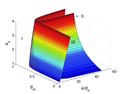
Figure 1: (Color online) Three dimensional phase diagram for the lysis-only model. Region I depends on the initial conditions to flow to the phage extinction or coexistence fixed point. Region II and III are basins of attraction for coexistence and phage extinction fixed points, respectively.

II.3 Discussion

As we can see, the bottom plane in Fig. 1 corresponds to the phase diagram in Weitz and Dushoff’s model, where $a_{n}=1.$ When

$$\alpha>\beta$$ (24)

leading to

$$a_{n}>1,$$ (25)

there is a shift in the phase diagram with a rapid shrinkage of the basin of attraction for region II, where any initial condition flows to the coexistence phase. The boundary between region I and III also moves to larger $\dfrac{\phi}{d_{n}},$ which implies that the more the good and poor metabolisms differ from each other in the progeny number, the easier the phages are driven out of the system. In order to see the effect of the phase shift more clearly, let us tune $a_{n}=1.3$ while keeping all the other parameters as those in Fig. 2 (I) in Weitz and Dushoff’s paperWeitz and Dushoff (2008) (Fig. 2). When $a_{n}=1,$ there is a neutral fixed point for coexistence. However, such a fixed point disappears (Fig. 3) when $a_{n}=1.3.$ The flow diagrams are generated by 4${}^{\text{th}}$ order Runge-Kutta method.

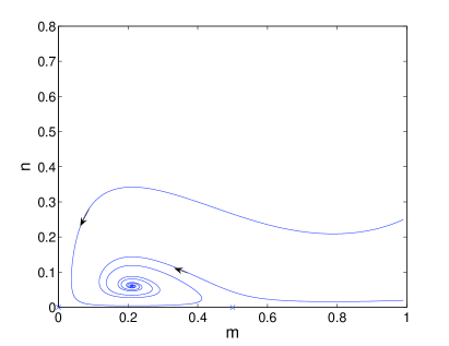
Figure 2: (Color online) Flow diagram for $a_{n}=1,\phi=5,d_{n}=1,d_{m}=0.1.$ “$\times$” denotes saddle points and “$\cdot$” is for stable fixed points.

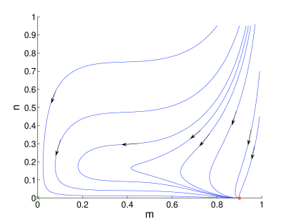
Figure 3: (Color online) Flow diagram for $a_{n}=1.3,\phi=5,d_{n}=1,d_{m}=0.1.$ “$\times$” denotes saddle points and “$\cdot$” is for stable fixed points.

In summary, we have obtained Weitz and Dushoff’s model by detailed derivation from the individual or microscopic level and found a small shift in the phase diagram. Such a shift, as we see, can be observed experimentally by the onset of coexistence for the two species.

III Lysogeny-lysis model

III.1 Derivation of the population dynamics from an individual-level model

Now we extend the lysis-only model above to incorporate lysogeny and investigate the important role of lysogeny in host-phage dynamics. Now there are three types of organism in the community. They are “healthy” hosts, which have no integration of phage genes, lysogens, and free phages, which live outside bacteria membranes. We will label “healthy” hosts, lysogens and free phages by $A$, $D$, and $B$, respectively, with population sizes $m$, $s$ and $n$. For the same reasons as in the lysis-only model, hosts and phages are thought of as being confined in different layers characterized by different carrying capacities. Hence both “healthy” hosts and lysogens are in the host layer with a total carrying capacity $K$. The empty sites in the host layer are denoted by $E$ and their number is $K-m-s$. In the phage layer, the empty sites are labelled by $\phi$ as before.

The incorporation of lysogens brings us more microscopic events. There are two pathways after phage infections: lysis and lysogeny. Immediate lysis for temperate phages is the same as virulent ones, which has been characterized by events in the previous section. Lysogeny is an option only for temperate phages, which will be investigated in detail here. First, there should be an event corresponding to lysogen formation, i.e. a phage integrates its DNA into the genome of the host and turns itself into a prophage. Second, lysogens will survive, replicate and die as “healthy” hosts. Last, environments might trigger prophage induction, which lyses the lysogen and releases the prophages inside. In all, there are eighteen microscopic events, which are listed in Table 3.

Table 3: Microscopic events in the lysogeny-lysis model.

description	symbols
birth of host	$AE\overset{b}{\rightarrow}AA$
	$DE\overset{b}{\rightarrow}DD$
death of host due to longevity	$A\overset{c}{\rightarrow}E$
	$D\overset{c}{\rightarrow}E$
death of host due to crowding	$AA\overset{d}{\rightarrow}AE$
	$DD\overset{d}{\rightarrow}DE$
	$AD\overset{\frac{1}{2}d}{\rightarrow}DE$
	$AD\overset{\frac{1}{2}d}{\rightarrow}AE$
host-phage interactions
$\cdot$ lysis under good metabolism	$AEB\overset{e}{\rightarrow}EE\alpha B$
$\cdot$ lysis under poor metabolism	$AAB\overset{f}{\rightarrow}EA\beta B$
	$ADB\overset{f}{\rightarrow}ED\beta B$
$\cdot$ lysogeny under good metabolism	$AEB\overset{h}{\rightarrow}DE$
$\cdot$ lysogeny under poor metabolism	$AAB\overset{k}{\rightarrow}DA$
	$ADB\overset{k}{\rightarrow}DD$
prophage induction
$\cdot$ under good metabolism	$DE\overset{p}{\rightarrow}EE\alpha B$
$\cdot$ under poor metabolism	$DD\overset{q}{\rightarrow}DE\beta B$
	$DA\overset{q}{\rightarrow}AE\beta B$
death of free phage	$B\overset{g}{\rightarrow}\phi$

Here $b$, $c$, $d$, $e$, $f$, $g$, $h$, $k$, $p$ and $q$ are constant reaction rates. $\alpha$ and $\beta$ are phage reproduction numbers under good and poor metabolisms, respectively. Although prophage induction enhances the survival ability for lysogens in several ways, such as suppressing the latter’s metabolismPaul (2008) through down-regulationChen et al. (2005), for simplicity we have assumed the same birth and death rates for “healthy” hosts and lysogens. We have the condition

$$\alpha>\beta,$$ (26)

as before. Furthermore, there are the following advantages under better metabolism: more successful and effective infection (Eq. (27a)), greater possibility to lyse the host (Eq. (27b)), and faster prophage release (Eq. (27c)). Since lysis is controlled by lytic repressor CI dimers while lysogeny is regulated by CII, we do not expect any special relationship between $e$ and $f$, and $p$ and $q$. These advantages can be expressed mathematically by the following inequalities:

$$e+h >f+k,$$ (27a)

$$\dfrac{e}{h} >\dfrac{f}{k},$$ (27b)

$$p >q.$$ (27c)

We draw events from the two layers the same way as in the lysis-only model and this results in the probabilities shown in Table 4.

From these events, we obtain the following evolution equations for all the three species after the calculations provided in Appendix B:

$$\dfrac{dm}{dt} =rm\left(1-\dfrac{m+s}{K}\right)-d_{1}m-\phi_{1}mn\left\{1-\dfrac{1}{K}\left[\left(1-a_{1}\right)m+\left(1-2a_{1}\right)s\right]\right\};$$ (28a)

$$\dfrac{ds}{dt} =rs\left(1-\dfrac{m+s}{K}\right)-d_{1}s+\phi_{2}mn\left\{1-\dfrac{1}{K}\left[\left(1-a_{21}\right)m+\left(1-2a_{21}\right)s\right]\right\}$$

$$\qquad-d_{2}s\left\{1-\dfrac{1}{K}[\left(1-2a_{22}\right)m+\left(1-a_{22}\right)s]\right\};$$ (28b)

$$\dfrac{dn}{dt} =\left[\left(\alpha-1\right)\phi_{1}-\alpha\phi_{2}\right]mn\left\{1-\dfrac{1}{K}\left[\left(1-a_{31}\right)m+\left(1-2a_{31}\right)s\right]\right\}$$

$$\qquad+\alpha d_{2}s\left\{1-\dfrac{1}{K}\left[\left(1-2a_{32}\right)m+\left(1-a_{32}\right)s\right]\right\}-d_{3}n;$$ (28c)

where

$$r =\dfrac{(2b+d)\mu\left(1-\nu\right)\left(1-\omega\right)}{K};$$ (29a)

$$d_{1} =\dfrac{(c\omega+d(1-\omega))\mu\left(1-\nu\right)}{K};$$ (29b)

$$d_{2} =\dfrac{2p\mu\left(1-\nu\right)\left(1-\omega\right)}{K};$$ (29c)

$$d_{3} =\dfrac{\left(1-\mu\right)\nu}{W};$$ (29d)

$$\phi_{1} =\dfrac{2(e+h)\mu\nu\left(1-\omega\right)}{KW};$$ (29e)

$$\phi_{2} =\dfrac{2h\mu\nu\left(1-\omega\right)}{KW};$$ (29f)

$$a_{1} =\dfrac{f+k}{2(e+h)};$$ (29g)

$$a_{21} =\dfrac{k}{2h};$$ (29h)

$$a_{22} =\dfrac{q}{2p};$$ (29i)

$$a_{31} =\dfrac{\beta f-k}{2(\alpha e-h)};$$ (29j)

$$a_{32} =\dfrac{\beta q}{2\alpha p}.$$ (29k)

Table 4: Probabilities for the combinations in the lysogeny-lysis model.

combination	probability
$AE$	$\mu\left(1-\nu\right)\left(1-\omega\right)\dfrac{2m\left(K-m-s\right)}{K\left(K-1\right)}$
$DE$	$\mu\left(1-\nu\right)\left(1-\omega\right)\dfrac{2s\left(K-m-s\right)}{K\left(K-1\right)}$
$A$	$\mu\left(1-\nu\right)\omega\dfrac{m}{K}$
$D$	$\mu\left(1-\nu\right)\omega\dfrac{s}{K}$
$AA$	$\mu\left(1-\nu\right)\left(1-\omega\right)\dfrac{m\left(m-1\right)}{K\left(K-1\right)}$
$DD$	$\mu\left(1-\nu\right)\left(1-\omega\right)\dfrac{s\left(s-1\right)}{K\left(K-1\right)}$
$AD$	$\mu\left(1-\nu\right)\left(1-\omega\right)\dfrac{2ms}{K\left(K-1\right)}$
$AEB$	$\mu\nu\left(1-\omega\right)\dfrac{2m\left(K-m-s\right)}{K\left(K-1\right)}\dfrac{n}{W}$
$AAB$	$\mu\nu\left(1-\omega\right)\dfrac{m\left(m-1\right)}{K\left(K-1\right)}\dfrac{n}{W}$
$ADB$	$\mu\nu\left(1-\omega\right)\dfrac{2ms}{K\left(K-1\right)}\dfrac{n}{W}$
$B$	$\left(1-\mu\right)\nu\dfrac{n}{W}$

We note that

$$\phi_{2} <\phi_{1};$$ (30)

$$0 <a_{1},a_{21},a_{22},a_{31},a_{32}<1;$$ (31)

$$a_{32} <a_{22}.$$ (32)

We also notice some kind of symmetry in the correction terms such as “$1-a_{1}$” and “$1-2a_{1}$”. $a_{1}$ originates from the poor metabolism of hosts $A$, which indirectly downshifts the efficiency of phage infection and synthesis. In equation (28a), “$a_{1}$” comes from the event $AAB\overset{f}{\rightarrow}EA\beta B,$ while “$2a_{1}$” is from $ADB\overset{f}{\rightarrow}ED\beta B.$ The factor “$2$” appears since “$AD$” is the same as “$DA$”.

Considering

$$\alpha\gg 1,$$ (33)

for example,

$$\alpha\approx 100$$ (34)

for lambda phagePtashne (2004), we approximate

$$\left(\alpha-1\right)\phi_{1}-\alpha\phi_{2}\approx\alpha\left(\phi_{1}-\phi_{2}\right).$$ (35)

Hence equation (28c) can be simplified as

$$\dfrac{dn}{dt}=\alpha\left(\phi_{1}-\phi_{2}\right)mn\left\{1-\dfrac{1}{K}\left[\left(1-a_{31}\right)m+\left(1-2a_{31}\right)s\right]\right\}+\alpha d_{2}s\left\{1-\dfrac{1}{K}\left[\left(1-2a_{32}\right)m+\left(1-a_{32}\right)s\right]\right\}-d_{3}n.$$ (36)

III.2 Results

In this section, we explore the predictions of the lysogeny-lysis model given by equations (28a), (28b) and (36).

Let

$$t^{\prime} =rt;$$ (37a)

$$\phi_{1}^{\prime} =\dfrac{\alpha\phi_{1}K}{r};$$ (37b)

$$\phi_{2}^{\prime} =\dfrac{\alpha\phi_{2}K}{r};$$ (37c)

$$d_{1}^{\prime} =\dfrac{d_{1}}{r};$$ (37d)

$$d_{2}^{\prime} =\dfrac{d_{2}}{r};$$ (37e)

$$d_{3}^{\prime} =\dfrac{d_{3}}{r};$$ (37f)

$$m^{\prime} =\dfrac{m}{K};$$ (37g)

$$s^{\prime} =\dfrac{s}{K};$$ (37h)

$$n^{\prime} =\dfrac{n}{\alpha K};$$ (37i)

and omitting the primes, the equations after non-dimensionalization become

$$\dfrac{dm}{dt} =m\left(1-m-s\right)-d_{1}m-\phi_{1}mn\left[1-\left(1-a_{1}\right)m-\left(1-2a_{1}\right)s\right];$$ (38a)

$$\dfrac{ds}{dt} =s\left(1-m-s\right)-d_{1}s+\phi_{2}mn\left[1-\left(1-a_{21}\right)m-\left(1-2a_{21}\right)s\right]-d_{2}s\left[1-\left(1-2a_{22}\right)m-\left(1-a_{22}\right)s\right];$$ (38b)

$$\dfrac{dn}{dt} =\left(\phi_{1}-\phi_{2}\right)mn\left[1-\left(1-a_{31}\right)m-\left(1-2a_{31}\right)s\right]+d_{2}s\left[1-\left(1-2a_{32}\right)m-\left(1-a_{32}\right)s\right]-d_{3}n.$$ (38c)

Formally, the fixed points can be solved by requiring that

$$\dfrac{dm}{dt} =0;$$ (39a)

$$\dfrac{ds}{dt} =0;$$ (39b)

$$\dfrac{dn}{dt} =0.$$ (39c)

However, we can only obtain four fixed points analytically. The first is the trivial case for the extinction of all the species

$$m =0;$$ (40a)

$$s =0;$$ (40b)

$$n =0.$$ (40c)

The second is the “healthy” host extinction fixed point

$$m =0;$$ (41a)

$$s =\dfrac{1-d_{1}-d_{2}}{1-d_{2}\left(1-a_{22}\right)};$$ (41b)

$$n =\dfrac{d_{2}}{d_{3}}s\left[1-\left(1-a_{32}\right)s\right].$$ (41c)

The third is the “healthy” host only fixed point

$$m =1-d_{1};$$ (42a)

$$s =0;$$ (42b)

$$n =0.$$ (42c)

The last is the lysogen extinction

$$m =\dfrac{1}{1-a_{21}};$$ (43a)

$$s =0;$$ (43b)

$$n =\dfrac{1-m-d_{1}}{\phi_{1}\left[1-\left(1-a_{1}\right)m\right]};$$ (43c)

whose existence requires that

$$\left(\phi_{1}-\phi_{2}\right)\left(a_{31}-a_{21}\right)=d_{3}\left(1-a_{21}\right)^{2}.$$ (44)

The more interesting coexistence of all the three species is hard to solve analytically since the order of the equations

$$m\left(1-m-s\right)-d_{1}m-\phi_{1}mn\left[1-\left(1-a_{1}\right)m-\left(1-2a_{1}\right)s\right] =0;$$ (45a)

$$s\left(1-m-s\right)-d_{1}s+\phi_{2}mn\left[1-\left(1-a_{21}\right)m-\left(1-2a_{21}\right)s\right]-d_{2}s\left[1-\left(1-2a_{22}\right)m-\left(1-a_{22}\right)s\right] =0;$$ (45b)

$$\left(\phi_{1}-\phi_{2}\right)mn\left[1-\left(1-a_{31}\right)m-\left(1-2a_{31}\right)s\right]+d_{2}s\left[1-\left(1-2a_{32}\right)m-\left(1-a_{32}\right)s\right]-d_{3}n =0;$$ (45c)

is too high. Using a 4${}^{\text{th}}$ order Runge-Kutta method, we found numerically a stable fixed point, shown in Fig. 4.

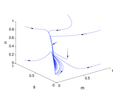
Figure 4: (Color online) In the lysogeny-lysis model, a stable fixed point for the coexistence of all the three species. The parameters are $\phi_{1}=1,\phi_{2}=0.8,d_{1}=0.5,d_{2}=0.49,d_{3}=0.1,a_{1}=a_{21}=a_{31}=0.1,a_{22}=a_{32}=0.5.$

III.3 Discussion

As shown in Eq. (38), there are, in total, ten parameters so that the phase space is difficult to visualize. We have studied the general trend of the transition between phases, starting with the dependence on phage mortality rate $d_{3}$. In Fig. 5, it is shown that when the phage mortality rate is low, the systems flows into a “healthy” host extinction phase. The phage population decreases with increase in the phage mortality rate, which is very reasonable physically. For intermediate values of $d_{3}$, there is coexistence for all the three species, while for large values of $d_{3}$, the only survival is “healthy” host, where all phages die out quickly out, leading to the extinction of lysogens.

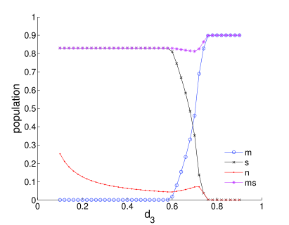
Figure 5: (Color online) The population of the community with increasing phage mortality rate $d_{3}.$ “$ms$” indicates the sum of $m$ and $s$.

We show the trend of the population with increasing lysis rate $d_{2}$ in Fig. 6. The phage prospers with the increase in the lysis rate, while the lysogen diminishes. The peak in the phage population appears when there is a balance in the number of lysogens available to lyse and the lysis rate. When the lysis rate is beyond the threshold at 0.54, lysogen number falls dramatically and there is a proliferation of “healthy” hosts. The total host population is roughly the same afterwards while the phage population upshifts a little with the increase in the “healthy” host available to infect but does not change further when the ratio between “healthy” hosts and lysogens converges.

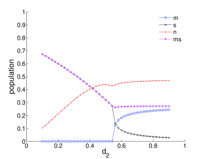
Figure 6: (Color online) The population for the community with the increase in the lysis rate $d_{2}.$

We have studied the effect of host mortality rate in Fig. 7. Obviously the total host population will fall monotonically when the hosts are more likely to die. We draw attention to the interesting peak in the phage population. When the host mortality rate is low, the phage population is suppressed due to the overcrowding of the lysogens, which degrades the metabolism and hence the infection and synthesis of phages. When the host mortality rate is high, on the other hand, the phages have insufficient hosts to infect and their population also declines.

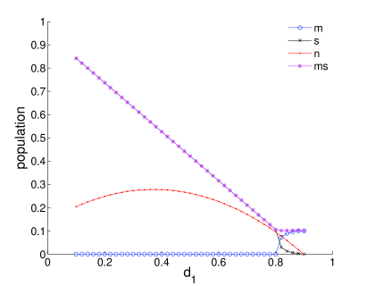
Figure 7: (Color online) The population for the community with the increase in the host mortality rate $d_{1}.$

III.4 Existence of a limit cycle

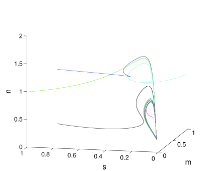
Figure 8: (Color online) A limit cycle in the flow diagram for different initial conditions with parameters $\phi_{1}=1,\phi_{2}=0.8,d_{1}=0.5,d_{2}=0.49,d_{3}=0.03,a_{1}=a_{21}=a_{31}=0.1,a_{22}=a_{32}=0.5.$

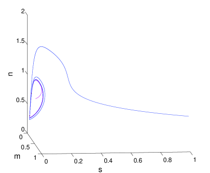
Figure 9: (Color online) A limit cycle in the flow diagram with different initial conditions for parameters $\phi_{1}=1,\phi_{2}=0.8,d_{1}=0.5,d_{2}=0.49,d_{3}=0.03,a_{1}=a_{21}=a_{31}=0.1,a_{22}=a_{32}=0.5$. The limit cycle is in a curved space. The blue curve initiated outside the cycle flows in while the red one from inside flows out.

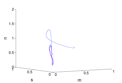
Figure 10: (Color online) A limit cycle in the flow diagram with different initial conditions for parameters $\phi_{1}=1,\phi_{2}=0.8,d_{1}=0.5,d_{2}=0.49,d_{3}=0.03,a_{1}=a_{21}=a_{31}=0.1,a_{22}=a_{32}=0.5$. The limit cycle is in a curved space.

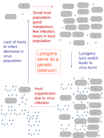
Figure 11: (Color online) Cartoon explanation for the limit cycle. When the population for host and phages are both small, the host will enjoy a boom because of good metabolism and little phage infection. Meanwhile prophages replicate with the fast reproduction of lysogens. Once the lysogeny-lysis switch is triggered, the destruction of lysogens will yield a huge virus burst. Then “healthy” host will encounter intensive phage infection and hence be suppressed. When most of the host die out, phage population shrinks quickly due to lack of infection. In this way, a cycle forms.

We have noticed that the dynamics exhibits a limit cycle for some combination of parameters (Fig. 8). In this section, we describe our numerical evidence for this assertion and present a plausible physical interpretation of our finding. In order to verify that it is a limit cycle instead of some unexpected slowing down near a putative stable or neutral fixed point, we have chosen an initial condition located inside the conjectured limit cycle. If there is, in fact, no real limit cycle, the dynamics will flow inwards no matter how slow it will be. However, as we can see in Fig. 9, the flow indicated by the red curve flows out. Hence we have observed in the flow diagram an oscillation in the population for all the three species. If we inspect neighboring time steps, it appears that the convergence is slow, since the deviation from step to step is very small. However, on longer time scales, we can see that the convergence is an illusion. Moreover, tilting the view angle, we see that the limit cycle is in some curved space instead of a single plane in Fig. 10. In order to investigate the emergence of the limit cycle, we have scanned part of the parameter space. For example, there is a stable coexistence fixed point for $d_{1}>0.41$ while $\phi_{1}=1,\phi_{2}=0.8,d_{2}=0.9,d_{3}=0.048,a_{1}=a_{21}=a_{31}=0.1$, and $a_{22}=a_{32}=0.5$. However, the above fixed point becomes unstable if $d_{1}<0.41$ leading to the limit cycle. As we see it, such an oscillation for the population in the community is a manifestation of the role of lysogens (Fig. 11). When the population for host and phages are both small, the host will enjoy a boom because of good metabolism and little phage infection. Meanwhile prophages replicate with the fast reproduction of lysogens. Once the lysogeny-lysis switch is triggered, the destruction of lysogens will yield a huge virus burst. Then “healthy” host will encounter intensive phage infection and hence be suppressed. When most of the host die out, phage population shrinks quickly due to lack of infection. In this way, a cycle forms. Integrating its DNA into the genome of a lysogen, a prophage is sheltered although it is temporarily dormant in the sense of viral infection. Such a stage assists prophages to survive demanding environmental conditions and provides an opportunity to resurrect the population when there are abundant “healthy” hosts. Thus lysogens are perfect genetic reservoirs for phages for potential future burstGoldenfeld and Woese (2007); Paul (2008).

IV Stochastic simulation

Up to now, all the calculations above were carried out within the scope of mean field theory. As a next step, it is important to see to what extent such predictions are disturbed by demographic fluctuations, and especially whether the limit cycle in the lysogeny-lysis model is stable. A second goal of this section is to link the parameters the parameters in our model to those which could characterize real experiments. In this section, we perform stochastic simulations using the Gillespie’s algorithmGillespie (1976, 1977), which is a very efficient strategy to simulate chemical reactions. The reaction rates ($b$, $c$, $d$,$e$, $f$ and $g$ in Table 1, and $b$, $c$, $d$, $e$, $f$, $g$, $h$, $k$, $p$ and $q$ in Table 3) are interpreted as average probability rates for the occurrence of the corresponding reactions in line with the Gillespie algorithm, where the effect of draw probability is incorporated automatically.

In the lysis-only model, the map between the two sets of parameters for reactions is

$$\widetilde{b} =bK;$$ (46a)

$$\widetilde{c} =c;$$ (46b)

$$\widetilde{d} =\frac{1}{2}dK;$$ (46c)

$$\widetilde{e} =eK;$$ (46d)

$$\widetilde{f} =\frac{1}{2}fK;$$ (46e)

$$\widetilde{g} =g;$$ (46f)

where tilde is used to indicate the probability rates in the Gillespie algorithm. Since there are more degrees of freedom in choosing microscopic event rates, different stochastic simulations may map into the same mean field phase diagram.

Our main interest is to explore the mean field limit cycle in the lysogeny-lysis model. We keep employing the tilde symbol to label the probability rates in the Gillespie sense and the map is

$$\widetilde{b} =bK;$$ (47a)

$$\widetilde{c} =c;$$ (47b)

$$\widetilde{d} =\frac{1}{2}dK;$$ (47c)

$$\widetilde{e} =eK;$$ (47d)

$$\widetilde{f} =\frac{1}{2}fK;$$ (47e)

$$\widetilde{h} =hK;$$ (47f)

$$\widetilde{k} =\frac{1}{2}kK;$$ (47g)

$$\widetilde{p} =pK;$$ (47h)

$$\widetilde{q} =\frac{1}{2}qK;$$ (47i)

$$\widetilde{g} =g.$$ (47j)

In Fig. 12, we show a limit cycle observed in our stochastic simulations. It is broadly consistent with the mean field predictions, as can be noted easily by the obvious similarities between Fig. 13 and Fig. 14, and Fig. 15 and Fig. 16 (when we project the three-dimensional phase space onto two dimensions), whose relationship is Eq. (37g), (37h) and (37i). As expected, we notice fluctuations in the stochastic simulation. For example, if Fig. 12 were shown in better resolution, we could see that the curve wiggled around the limit cycle. Usually fluctuation is two orders of magnitude smaller than the value it wiggles. Hence we conclude that the limit cycle is inherent to the model and robust to stochastic fluctuations, which serves to confirm the essential role of lysogens in stabilizing the cycling in the populations.

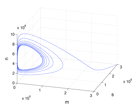
Figure 12: A limit cycle in the phase space with parameters in the Gillespie algorithm $\widetilde{b}=0.4,\widetilde{c}=0.1,\widetilde{d}=0.2,\widetilde{e}=1.2\times 10^{-10},\widetilde{f}=1.2\times 10^{-11},\widetilde{g}=0.018,\widetilde{h}=4.8\times 10^{-10},\widetilde{k}=4.8\times 10^{-11},\widetilde{p}=0.54$, and $\widetilde{q}=0.27$.

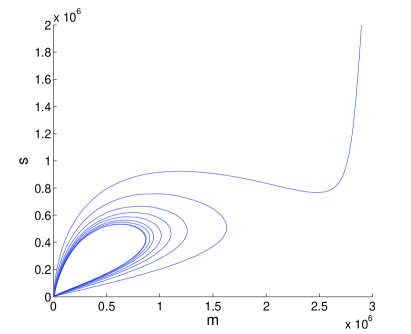
Figure 13: The projection of Fig. 12 onto the m-s plane.

Figure 14: A limit cycle projected onto m-s plane in the mean field theory with parameters $\phi_{1}=1,\phi_{2}=0.8,d_{1}=0.5,d_{2}=0.9,d_{3}=0.03,a_{1}=a_{21}=a_{31}=0.1$, and $a_{22}=a_{32}=0.5.$

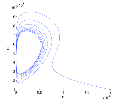
Figure 15: The projection of Fig. 12 onto the s-n plane.

Figure 16: A limit cycle projected onto the s-n plane in the mean field theory with parameters $\phi_{1}=1,\phi_{2}=0.8,d_{1}=0.5,d_{2}=0.9,d_{3}=0.03,a_{1}=a_{21}=a_{31}=0.1$, and $a_{22}=a_{32}=0.5.$

V Parameters in the model

Up to this point, all the parameters above or their values we have explored are difficult to relate to experiment. The purpose of this section is to bridge the gap.

The birth rate of the host $b$ is medium-dependent. Usually the expression of Lac proteins is highly suppressed by Lac repressors in a lacose-free medium to optimize energy investment and metabolism of the bacteria. In the above two models, we have categorized the death of the hosts to longevity and crowding. In fact, it is hard to mark a watershed clearly. Instead, what is observed is a population-dependent growth rate, which is a combined effect of $b$, $c$ and $d$. Herein, the rate $d$ for the death of the host due to crowding is introduced artificially to account for the actual population dependence. Thus, we are justified in assuming that the death rate of the host due to longevity $c$, which incorporates other physical and non-density-dependent factors, is fixed with the variation in host population. The growth rate for E. coli may drop to $0.2$ h^-1 at $37^{\circ}$C when glycolate serves as the carbon source but usually is in the range from $0.5$ h^-1 to $2.0$ h^-1Marr (1991); Hadas et al. (1997). The growth rate is species- and strain-specific, which for Pseudoalteromonas sp. strain SKA18 (accessible number AF188330 in GenBank)Middelboe (2000), for example, is an order of magnitude smaller. Similarly, lysis rate $f$, lysogeny rate $k$, prophage induction rate $q$, and replicate number per capita $\beta$, which are all under poor metabolism, are introduced manually to characterize the population-dependent feature of the interactions in order to leave their population-independent counterparts $e$, $h$, $p$ and $\alpha$ fixed. In the case of virulent phages, such as one in the family SiphoviridaeMiddelboe et al. (2001) attacking Pseudoalteromonas sp. strain SKA18Middelboe (2000), corresponding to the lysis-only model, the reported lysis rate spans from $0.2$ to $2.0$ h^-1 subject to the growth rate of the bacteria so that we can estimate $e$ to be on the order of $1.0$ h^-1 and $f$ to be an order of magnitude smaller than $e$.

For temperate phages in the lysogeny-lysis model, the spontaneous lysis rate is far smaller, being of the order of $10^{-9}$ to $10^{-7}$ per generation per cellAurell et al. (2002). The percentage of lysogens is assayed through prophage induction by the addition of mitomycin C, UV radiation or other environmental conditions that may inhibit lambda phage repressors. Under good metabolism the lysogeny rate $h$ for $\lambda$ phage infecting E. coli and prophage induction rate are on the order of $1$ h^-1 and $2$ h^-1, respectivelyKourilsky (1971). Their counterparts under poor metabolism are estimated to be one or two orders of magnitude smaller. For instance, the prophage induction rate for log-phase marine lysogensJiang and Paul (1998) is on the order of $0.03$ h^-1. Replicate number per capita $\alpha$ is about $100$ for phage $\lambda$Ptashne (2004), and may be up to $600$ for phage W-14Kropinski and Warren (1970), while $\beta$ is about 20 or 30 for both. The death of free phage is quite rare, which may result from the cleavage by proteins and depends on physical conditions such as temperature, humidity and pH values. C. D. Jepson and J. B. MarchJepson and March (2004) reported that phage $\lambda$ is highly stable, whose half life in suspension ranges from 2.3 days at $4.2^{\circ}$C to 36 days at $20^{\circ}$C. Even if we take the half life be one day, the corresponding death rate $g$ is on the order of $10^{-6}$ per second and can be suppressed by cooling down. Actually, the loss of free phage in nature, to a great extent, is through diffusion since bacteria are more immobile due to their large particle size compared to that of phages. In laboratory, the death rate can be manipulated through continuous dilution and washing out, and a wide range of death rates can be realized.

When all the parameters are tuned properly, the limit cycle in the lysogeny-lysis model is observable in experiment. We estimate the period of the limit cycle to be on the order of days. Take Fig. 13 as an example. A cycle there is composed of about $10,000$ computational steps, in other words $10,000$ events, which corresponds to about $120$ [time unit] in the simulation. In Fig. 13 the birth rate is $0.4$ [time unit]^-1, while in the real world the life cycle of an E. coli in good laboratory conditions, for example, is about half an hour, which is $2$ hour ^-1. Hence the cycle is $120\times 0.4/2=24$ hours, which is one day.

VI Conclusion

We have derived the mean field population dynamics for host-phage communities both without and with lysogens. In the lysis-only model, we successfully obtained a description similar to the starting point assumed by Weitz and DushoffWeitz and Dushoff (2008), and we found that the phase diagram was modified only slightly to the difference in good and poor metabolism. In the lysogeny-lysis model, we identified the asymptotic states, which included not only coexistence and extinction fixed points, but population cycling of all microbes, lysogens and phagess. Our findings support the notion that lysogens act as a reservoir and are in principle amenable to experimental verification. We simulated the stochastic process using the Gillespie algorithm and verified the robustness of our results to fluctuations, and especially demonstrated the stability of the limit cycle.

Although complicated, our model inevitably makes some drastic assumptions, in addition to the most severe of all—the omission of spatial structure. In particular, we treat “healthy” hosts and lysogens in the same way regarding their natural birth, death and crowding effect. However, experimentally, the expression of prophage genes and the control of host gene expression by viral genes seem to impart to lysogens econominization in their metabolismPaul (2008). When unnecessary metabolic activities are suppressed, lysogens optimize their energy expenses and therefore gain some survival advantage compared to “healthy” hosts in unfavorable conditions, which suggests that the natural birth, death and crowding effects of lysogens are distinct from those of “healthy” hosts. Hence our model is a minimal model that can capture the non-trivial role of lysogens in the population dynamics of microbe-phage communities, in addition to the usual predator-prey interactions.

This work can be extended in several ways, but perhaps the most interesting are those which relate to the evolution of the field of genes distributed amongst the microbes, viruses and lysogens. Lysogens are genome carriers of not only microbes but also prophages, capable of yielding virus bursts when triggered by environmental stress. In this way, the role of lysogens and viruses as a reservoir of genes is mediated through phage infection and the lysogeny-lysis switch by the metabolism of the host. The metabolism of the host is, in turn, to a great extent influenced by environmental conditions. Thus, this model is a starting point for ecology-mediated evolution. It is also useful to stress that each individual microbe or virus constitutes a part of another organism’s environment. Thus, the effects which our work begins to treat, represent a microcosm of the intricate interplay between ecology and evolution in microbe-virus communities.

Appendix A Transition matrices for the lysis-only model

Here we provide the transition matrices, which are the probabilities for the change in the population in each time step in the lysis-only model.

$$T\left(m+1,n|m,n\right)=b\mu\left(1-\nu\right)\left(1-\omega\right)\dfrac{2m\left(K-m\right)}{K\left(K-1\right)}=\widetilde{b}m\left(1-\dfrac{m}{K}\right);$$ (48)

$$\widetilde{b}=\dfrac{2b\mu\left(1-\nu\right)\left(1-\omega\right)}{K-1}\approx\dfrac{2b\mu\left(1-\nu\right)\left(1-\omega\right)}{K};$$ (49)

$$T\left(m-1,n|m,n\right)=c\mu\left(1-\nu\right)\omega\dfrac{m}{K}+d\mu\left(1-\nu\right)\left(1-\omega\right)\dfrac{m\left(m-1\right)}{K\left(K-1\right)}=\widetilde{c}m+\widetilde{d}m\left(\dfrac{m}{K}-\dfrac{1}{K}\right)\approx\widetilde{c}m+\widetilde{d}\dfrac{m^{2}}{K};$$ (50)

$$\widetilde{c}=\dfrac{c\mu\left(1-\nu\right)\omega}{K};$$ (51)

$$\widetilde{d}=\dfrac{d\mu\left(1-\nu\right)\left(1-\omega\right)}{K-1}\approx\dfrac{d\mu\left(1-\nu\right)\left(1-\omega\right)}{K};$$ (52)

$$T\left(m-1,n+\alpha-1|m,n\right)=e\mu\nu\left(1-\omega\right)\dfrac{2m\left(K-m\right)}{K\left(K-1\right)}\dfrac{n}{W}=\widetilde{e}mn\left(1-\dfrac{m}{K}\right);$$ (53)

$$\widetilde{e}=\dfrac{2e\mu\nu\left(1-\omega\right)}{\left(K-1\right)W}\approx\dfrac{2e\mu\nu\left(1-\omega\right)}{KW}.$$ (54)

$$T\left(m-1,n+\beta-1|m,n\right)=f\mu\nu\left(1-\omega\right)\dfrac{m\left(m-1\right)}{K\left(K-1\right)}\dfrac{n}{W}=\widetilde{f}\dfrac{m^{2}n}{K};$$ (55)

$$\widetilde{f}=\dfrac{f\mu\nu\left(1-\omega\right)}{\left(K-1\right)W}\approx\dfrac{f\mu\nu\left(1-\omega\right)}{KW}.$$ (56)

$$T\left(m,n-1|m,n\right)=g\left(1-\mu\right)\nu\dfrac{n}{W}=\widetilde{g}n;$$ (57)

$$\widetilde{g}=\dfrac{\left(1-\mu\right)\nu}{W}.$$ (58)

All the other transition matrixes are zero. Noting that all the events in Table 1 are Markov processes, we know that the time evolution for the probability with $m$ hosts and $n$ phages at time $t$ will be

$$\dfrac{d}{dt}P\left(m,n,t\right)=T\left(m,n|m-1,n\right)P\left(m-1,n,t\right)+T\left(m,n|m+1,n\right)P\left(m+1,n,t\right)$$

$$+T\left(m,n|m+1,n+\alpha-1\right)P\left(m+1,n+\alpha-1,t\right)+T\left(m,n|m+1,n+\beta-1\right)P\left(m+1,n+\beta-1,t\right)$$

$$+T\left(m,n|m,n+1\right)P\left(m,n+1,t\right)-[T\left(m+1,n|m,n\right)+T\left(m-1,n|m,n\right)+T\left(m-1,n+\alpha-1|m,n\right)$$

$$+T\left(m-1,n+\beta-1|m,n\right)+T\left(m,n-1|m,n\right)]P\left(m-1,n,t\right).$$ (59)

Applying summations according to Eq. (3), we will get

$$\dfrac{d\left\langle m\right\rangle}{dt} =\left\langle T\left(m+1,n|m,n\right)\right\rangle-\left\langle T\left(m-1,n|m,n\right)\right\rangle$$

$$\qquad-\left\langle T\left(m-1,n+\alpha-1|m,n\right)\right\rangle$$

$$\qquad-\left\langle T\left(m-1,n+\beta-1|m,n\right)\right\rangle$$

$$\approx\left(\widetilde{b}+\widetilde{d}\right)\left\langle m\right\rangle\left(1-\dfrac{\left\langle m\right\rangle}{K}\right)-\left(\widetilde{c}+\widetilde{d}\right)\left\langle m\right\rangle$$

$$\qquad-\widetilde{e}\left\langle m\right\rangle\left\langle n\right\rangle\left[1-\left(1-\dfrac{\widetilde{f}}{\widetilde{e}}\right)\dfrac{\left\langle m\right\rangle}{K}\right];$$ (60a)

$$\dfrac{d\left\langle n\right\rangle}{dt} =\left(\alpha-1\right)\left\langle T\left(m-1,n+\alpha-1|m,n\right)\right\rangle$$

$$\qquad+\left(\beta-1\right)\left\langle T\left(m-1,n+\beta-1|m,n\right)\right\rangle$$

$$\qquad-\left\langle T\left(m,n-1|m,n\right)\right\rangle$$

$$=\left(\alpha-1\right)\ \widetilde{e}\left\langle m\right\rangle\left\langle n\right\rangle\left[1-\left(1-\dfrac{\left(\beta-1\right)\widetilde{f}}{\left(\alpha-1\right)\widetilde{e}}\right)\dfrac{\left\langle m\right\rangle}{K}\right]$$

$$\qquad-\widetilde{g}\left\langle n\right\rangle.$$ (60b)

Let

$$r =\widetilde{b}+\widetilde{d};$$ (61a)

$$\phi =\widetilde{e};$$ (61b)

$$\gamma =\alpha-1;$$ (61c)

$$d_{m} =\widetilde{c}+\widetilde{d};$$ (61d)

$$d_{n} =\widetilde{g};$$ (61e)

$$a_{m} =1-\dfrac{\widetilde{f}}{\widetilde{e}};$$ (61f)

$$a_{n} =1-\dfrac{\left(\beta-1\right)\widetilde{f}}{\left(\alpha-1\right)\widetilde{e}};$$ (61g)

which is Eq. (6), we can arrive at Eq. (5).

Appendix B Transition matrices for the lysogeny-lysis model

In this appendix, we provide details for the derivations of the lysogeny-lysis model.

According to Table 3 and Table 4, we can obtain the following non-zero transition matrixes:

$$T\left(m+1,s,n|m,s,n\right)=b\mu\left(1-\nu\right)\left(1-\omega\right)\dfrac{2m\left(K-m-s\right)}{K\left(K-1\right)}=\widetilde{b}m\left(1-\dfrac{m+s}{K}\right);$$ (62)

$$\widetilde{b}=\dfrac{2b\mu\left(1-\nu\right)\left(1-\omega\right)}{K-1}\approx\dfrac{2b\mu\left(1-\nu\right)\left(1-\omega\right)}{K}.$$ (63)

$$T\left(m,s+1,n|m,s,n\right)=b\mu\left(1-\nu\right)\left(1-\omega\right)\dfrac{2s\left(K-m-s\right)}{K\left(K-1\right)}=\widetilde{b}s\left(1-\dfrac{m+s}{K}\right);$$ (64)

$$T\left(m-1,s,n|m,s,n\right) =c\mu\left(1-\nu\right)\omega\dfrac{m}{K}+d\mu\left(1-\nu\right)\left(1-\omega\right)\dfrac{m\left(m-1\right)}{K\left(K-1\right)}+\dfrac{1}{2}d\mu\left(1-\nu\right)\left(1-\omega\right)\dfrac{2ms}{K\left(K-1\right)}$$

$$=\widetilde{c}m+\widetilde{d}m\dfrac{m+s}{K}.$$ (65)

$$\widetilde{c}=\dfrac{c\mu\left(1-\nu\right)\omega}{K};$$ (66)

$$\widetilde{d}=\dfrac{d\mu\left(1-\nu\right)\left(1-\omega\right)}{K-1}\approx\dfrac{d\mu\left(1-\nu\right)\left(1-\omega\right)}{K}.$$ (67)

$$T\left(m,s-1,n|m,s,n\right) =c\mu\left(1-\nu\right)\omega\dfrac{s}{K}+d\mu\left(1-\nu\right)\left(1-\omega\right)\dfrac{s\left(s-1\right)}{K\left(K-1\right)}+\dfrac{1}{2}d\mu\left(1-\nu\right)\left(1-\omega\right)\dfrac{2ms}{K\left(K-1\right)}$$

$$=\widetilde{c}s+\widetilde{d}s\dfrac{m+s}{K}.$$ (68)

$$T\left(m-1,s,n+\alpha+1|m,s,n\right)=e\mu\nu\left(1-\omega\right)\dfrac{2m\left(K-m-s\right)}{K\left(K-1\right)}\dfrac{n}{W}=\widetilde{e}mn\left(1-\dfrac{m+s}{K}\right);$$ (69)

$$\widetilde{e}=\dfrac{2e\mu\nu\left(1-\omega\right)}{\left(K-1\right)W}\approx\dfrac{2e\mu\nu\left(1-\omega\right)}{KW}.$$ (70)

$$T\left(m-1,s,n+\beta+1|m,s,n\right)=f\mu\nu\left(1-\omega\right)\dfrac{m\left(m-1\right)}{K\left(K-1\right)}\dfrac{n}{W}+f\mu\nu\left(1-\omega\right)\dfrac{2ms}{K\left(K-1\right)}\dfrac{n}{W}=\widetilde{f}mn\dfrac{m+2s}{K};$$ (71)

$$\widetilde{f}=\dfrac{f\mu\nu\left(1-\omega\right)}{\left(K-1\right)W}\approx\dfrac{f\mu\nu\left(1-\omega\right)}{KW}.$$ (72)

$$T\left(m-1,s+1,n-1|m,s,n\right)=h\mu\nu\left(1-\omega\right)\dfrac{2m\left(K-m-s\right)}{K\left(K-1\right)}\dfrac{n}{W}+k\mu\nu\left(1-\omega\right)\dfrac{m\left(m-1\right)}{K\left(K-1\right)}\dfrac{n}{W}$$

$$+k\mu\nu\left(1-\omega\right)\dfrac{2ms}{K\left(K-1\right)}\dfrac{n}{W}=\widetilde{h}mn\left(1-\dfrac{m+s}{K}\right)+\widetilde{k}mn\dfrac{m+2s}{K};$$ (73)

$$\widetilde{h}=\dfrac{2h\mu\nu\left(1-\omega\right)}{\left(K-1\right)W}\approx\dfrac{2h\mu\nu\left(1-\omega\right)}{KW};$$ (74)

$$\widetilde{k}=\dfrac{k\mu\nu\left(1-\omega\right)}{\left(K-1\right)W}\approx\dfrac{k\mu\nu\left(1-\omega\right)}{KW}.$$ (75)

$$T\left(m,s-1,n+\alpha|m,s,n\right)=p\mu\left(1-\nu\right)\left(1-\omega\right)\dfrac{2s\left(K-m-s\right)}{K\left(K-1\right)}=\widetilde{p}s\left(1-\dfrac{m+s}{K}\right);$$ (76)

$$\widetilde{p}=\dfrac{2p\mu\left(1-\nu\right)\left(1-\omega\right)}{K-1}\approx\dfrac{2p\mu\left(1-\nu\right)\left(1-\omega\right)}{K}.$$ (77)

$$T\left(m,s-1,n+\beta|m,s,n\right)=q\mu\left(1-\nu\right)\left(1-\omega\right)\dfrac{s\left(s-1\right)}{K\left(K-1\right)}+q\mu\left(1-\nu\right)\left(1-\omega\right)\dfrac{2ms}{K\left(K-1\right)}=\widetilde{q}s\dfrac{2m+s}{K};$$ (78)

$$\widetilde{q}=\dfrac{q\mu\left(1-\nu\right)\left(1-\omega\right)}{K-1}\approx\dfrac{q\mu\left(1-\nu\right)\left(1-\omega\right)}{K}.$$ (79)

$$T\left(m,s,n-1|m,s,n\right)=g\left(1-\mu\right)\nu\dfrac{n}{W}=\widetilde{g}n;$$ (80)

$$\widetilde{g}=\dfrac{\left(1-\mu\right)\nu}{W}.$$ (81)

Ignoring fluctuations and correlations, we derive the populations dynamics at the mean field level. The time evolution for population size is

$$\dfrac{d\left\langle m\right\rangle}{dt} =\left\langle T\left(m+1,s,n|m,s,n\right)\right\rangle-\left\langle T\left(m-1,s,n|m,s,n\right)\right\rangle-\left\langle T\left(m-1,s,n+\alpha-1|m,s,n\right)\right\rangle$$

$$\qquad-\left\langle T\left(m-1,s,n+\beta-1|m,s,n\right)\right\rangle-\left\langle T\left(m-1,s+1,n-1|m,s,n\right)\right\rangle$$

$$=\left(\widetilde{b}+\widetilde{d}\right)\left\langle m\right\rangle\left(1-\dfrac{\left\langle m\right\rangle+\left\langle s\right\rangle}{K}\right)-\left(\widetilde{c}+\widetilde{d}\right)\left\langle m\right\rangle$$

$$\qquad-\left(\widetilde{e}+\widetilde{h}\right)\left\langle m\right\rangle\left\langle n\right\rangle\left\{1-\dfrac{1}{K}\left[\left(1-\dfrac{\widetilde{f}+\widetilde{k}}{\widetilde{e}+\widetilde{h}}\right)\left\langle m\right\rangle+\left(1-2\cdot\dfrac{\widetilde{f}+\widetilde{k}}{\widetilde{e}+\widetilde{h}}\right)\left\langle s\right\rangle\right]\right\};$$ (82a)

$$\dfrac{d\left\langle s\right\rangle}{dt} =\left\langle T\left(m,s+1,n|m,s,n\right)\right\rangle-\left\langle T\left(m,s-1,n|m,s,n\right)\right\rangle+\left\langle T\left(m-1,s+1,n-1|m,s,n\right)\right\rangle$$

$$\qquad-\left\langle T\left(m,s-1,n+\alpha|m,s,n\right)\right\rangle-\left\langle T\left(m,s-1,n+\beta|m,s,n\right)\right\rangle$$

$$=\left(\widetilde{b}+\widetilde{d}\right)\left\langle s\right\rangle\left(1-\dfrac{\left\langle m\right\rangle+\left\langle s\right\rangle}{K}\right)-\left(\widetilde{c}+\widetilde{d}\right)\left\langle s\right\rangle$$

$$\qquad-\widetilde{h}\left\langle m\right\rangle\left\langle n\right\rangle\left\{1-\dfrac{1}{K}\left[\left(1-\dfrac{\widetilde{k}}{\widetilde{h}}\right)\left\langle m\right\rangle+\left(1-2\cdot\dfrac{\widetilde{k}}{\widetilde{h}}\right)\left\langle s\right\rangle\right]\right\}$$

$$\qquad-\widetilde{p}\left\langle s\right\rangle\left\{1-\dfrac{1}{K}\left[\left(1-2\cdot\dfrac{\widetilde{q}}{\widetilde{p}}\right)\left\langle m\right\rangle+\left(1-\dfrac{\widetilde{q}}{\widetilde{p}}\right)\left\langle s\right\rangle\right]\right\};$$ (82b)

$$\dfrac{d\left\langle n\right\rangle}{dt} =\left(\alpha-1\right)\left\langle T\left(m-1,s,n+\alpha-1|m,s,n\right)\right\rangle+\left(\beta-1\right)\left\langle T\left(m-1,s,n+\beta-1|m,s,n\right)\right\rangle$$

$$\qquad-\left\langle T\left(m-1,s+1,n-1|m,s,n\right)\right\rangle+\alpha\left\langle T\left(m,s-1,n+\alpha|m,s,n\right)\right\rangle+\beta\left\langle T\left(m,s-1,n+\beta|m,s,n\right)\right\rangle$$

$$\qquad-\left\langle T\left(m,s,n-1|m,s,n\right)\right\rangle$$

$$=\left[\left(\alpha-1\right)\widetilde{e}-\widetilde{h}\right]\left\langle m\right\rangle\left\langle n\right\rangle\left\{1-\dfrac{1}{K}\left[\left(1-\dfrac{\left(\beta-1\right)\widetilde{f}-\widetilde{k}}{\left(\alpha-1\right)\widetilde{e}-\widetilde{h}}\right)\left\langle m\right\rangle+\left(1-2\cdot\dfrac{\left(\beta-1\right)\widetilde{f}-\widetilde{k}}{\left(\alpha-1\right)\widetilde{e}-\widetilde{h}}\right)\left\langle s\right\rangle\right]\right\}$$

$$\qquad+\alpha\widetilde{p}\left\langle s\right\rangle\left\{1-\dfrac{1}{K}\left[\left(1-2\cdot\dfrac{\beta\widetilde{q}}{\alpha\widetilde{p}}\right)\left\langle m\right\rangle+\left(1-\dfrac{\beta\widetilde{q}}{\alpha\widetilde{p}}\right)\left\langle s\right\rangle\right]\right\}-\widetilde{g}\left\langle n\right\rangle.$$ (82c)

Let

$$r =\widetilde{b}+\widetilde{d};$$ (83a)

$$d_{1} =\widetilde{c}+\widetilde{d};$$ (83b)

$$d_{2} =\widetilde{p};$$ (83c)

$$d_{3} =\widetilde{g};$$ (83d)

$$\phi_{1} =\widetilde{e}+\widetilde{h};$$ (83e)

$$\phi_{2} =\widetilde{h};$$ (83f)

$$a_{1} =\dfrac{\widetilde{f}+\widetilde{k}}{\widetilde{e}+\widetilde{h}};$$ (83g)

$$a_{21} =\dfrac{\widetilde{k}}{\widetilde{h}};$$ (83h)

$$a_{22} =\dfrac{\widetilde{q}}{\widetilde{p}};$$ (83i)

$$a_{31} =\dfrac{\left(\beta-1\right)\widetilde{f}-\widetilde{k}}{\left(\alpha-1\right)\widetilde{e}-\widetilde{h}};$$ (83j)

$$a_{32} =\dfrac{\beta\widetilde{q}}{\alpha\widetilde{p}};$$ (83k)

which is Eq. (29), and omit angle-brackets for simplicity, Eq. (82) can be written as Eq. (28).