Antiferromagnetic Spinor Condensates are Quantum Rotors

Abstract

We establish a theoretical correspondence between spin-one antiferromagnetic spinor condensates in an external magnetic field and quantum rotor models in an external potential. We show that the rotor model provides a conceptually clear picture of the possible phases and dynamical regimes of the antiferromagnetic condensate. We also show that this mapping simplifies calculations of the condensate’s spectrum and wavefunctions. We use the rotor mapping to describe the different dynamical regimes recently observed in ²³Na condensates Liu et al. (2009a, b). We also suggest a way to experimentally observe quantum mechanical effects (collapse and revival) in spinor condensates.

Bose-Einstein condensates occurring in ultracold atoms having internal spin degrees of freedom, the so-called spinor condensates, offer an exciting addition to the family of quantum many body spin systems realizable in the laboratory Stenger et al. (1998). Of particular interest are the long coherence times and small dissipation rates which allow access to dynamical regimes not available in the solid state. Recently there has been considerable experimental progress in elucidating the dynamics of spinor condensates. Such endeavors include dynamics experiments on ⁸⁷Rb atoms for the hyperfine spin-one Chang et al. (2005); Sadler et al. (2006) and spin-two Klempt et al. (2009) manifolds as well as, most recently, experiments on ²³Na condensates Liu et al. (2009a, b). ²³Na spin-one condensates are qualitatively different than their ⁸⁷Rb counterpart due to antiferromagnetic interactions. This leads to ground states having zero spin moment as well as disparate dynamical regimes.

The NIST experiments Liu et al. (2009a, b) were performed in a trapping potential sufficiently tight such that, within a good approximation, the bosonic atoms all occupy the same spatial mode. This allows the spin dynamics of the system, which is often obscured by spatial variations, to be directly probed. The condensate was prepared in an initial unstable ferromagnetic state and then allowed to evolve freely in time. For small magnetic fields, the system oscillates about the ferromagnetic state, never reaching zero spin moment $\langle{\bf F}\rangle=0$ at any time. On the other hand, when the magnetic field exceeds a critical value the system evolves through $\langle{\bf F}\rangle=0$ reaching a state pointing in the opposite direction and back periodically, the so-called “running phase” trajectories. It was shown that these different regimes could be interpreted as being on different sides of a separatrix in the phase space of the mean-field energy of the system Liu et al. (2009a, b).

In the single-mode approximation, the full quantum Hamiltonian of the system is

$$H=\frac{g}{2N}F^{2}-qa_{0}^{\dagger}a_{0}.$$ (1)

Here, ${\bf F}=a^{\dagger}_{\alpha}{\bf F}_{\alpha\beta}a_{\beta}$ is the total spin operator where ${\bf F}_{\alpha\beta}$ are the spin-one matrices and $a_{1},a_{0},a_{-1}$ are bosonic annihilation operators for each spin state, $N$ is the total particle number, $g$ is the spin-dependent interaction, and $q$ is the quadratic Zeeman shift due to an external magnetic field fn . When $q=0$ the exact ground state of the above Hamiltonian is a condensate of singlet pairs of bosons given by Law et al. (1998)

$$|{S}\rangle=\left(a_{0}^{\dagger}a_{0}^{\dagger}-2a_{1}^{\dagger}a_{-1}^{\dagger}\right)^{N/2}|{0}\rangle.$$ (2)

This ground state is unique and breaks no symmetries. However, for large particle numbers, this state becomes extremely delicate, being unstable to small external magnetic fields. Thus the observed phases for most experimental antiferromagnetic systems are more appropriately described by symmetry-broken nematic states which are well-described by mean-field theory Ho (1998); Ohmi and Machida (1998). This is reminiscent of Anderson’s “tower of states” argument for Néel ordering in solid state quantum antiferromagnets, despite the fact that the true ground state for finite-size bipartite lattices can be shown to be a spin singlet Auerbach (New York, 1994).

In this Letter, we develop a conceptually new approach to describe the quantum dynamics of antiferromagnetic spinor condensates. In particular, we map the Hamiltonian in Eq. (1) onto a quantum rotor Hamiltonian

$${\mathscr{H}}=\frac{1}{2I}L^{2}+V(\theta)$$ (3)

where ${\bf L}$ is the angular momentum of the rotor, $I=N\hbar^{2}/g$ is the moment of inertia, and $V(\theta)=q\left(N+\frac{3}{2}\right)\sin^{2}(\theta)+\frac{q^{2}N}{8g}\sin^{2}(2\theta)$ is the external potential. The mapping is exact in the sense that the complete spectrum of Eq. (1) for $N$ bosons precisely agrees with the lowest set of eigenvalues of Eq. (3) (which has an unbounded spectrum from above). A similar procedure has been used to derive an exact phase model describing bosons in a double-well potential Anglin et al. (2001). One can see that the singlet state of paired bosons, Eq. (2), corresponds to a state where the rotor is delocalized over the entire sphere while the symmetry-broken nematic state corresponds to the rotor being in a position eigenstate. We will show how Eq. (3) can be used to obtain simple expressions for the spectrum and wavefunction of the spinor condensate. We then show how the semiclassical limit of the rotor system provides a natural interpretation of the dynamical regimes of anti-ferromagnetic spinor condensates observed experimentally Liu et al. (2009a, b). Finally, we make a prediction to observe quantum mechanical effects (i.e. non-mean field effects) in spinor condensates which have so far eluded experimental detection. Specifically, we show that the abrupt removal of a magnetic field used to prepare the system in a nematic state will lead to collapse and revival dynamics, which cannot be explained with mean field theory alone.

We now proceed with the main technical advance of this work: an exact mapping of Eq. (1) onto an effective rotor Hamiltonian, thus establishing that antiferromagnetic spinor condensates are effective realizations of the quantum rotor model. It is most useful to express the bosonic creation and annihilation operators as quantities that transform as cartesian vectors under rotations. To that end we define the operators $b_{x}=-(a_{1}-a_{-1})/\sqrt{2},$ $b_{y}=(a_{1}+a_{-1})/i\sqrt{2},$ and $b_{z}=a_{0}$ which satisfy bosonic commutation relations. It is then straightforward to express the Hamiltonian Eq. (1) in terms of these operators. Specifically, the spin operator is ${\bf F}=-i{\bf b}^{\dagger}\times{\bf b}$ while the quadratic Zeeman shift is $b_{z}^{\dagger}b_{z}$. With these operators we construct the complete set of states

$$|{{\bf\Omega}_{N}}\rangle\equiv\frac{1}{\sqrt{N!}}\left({\bf\Omega}\cdot{\bf b}^{\dagger}\right)^{N}|{0}\rangle$$ (4)

where ${\bf\Omega}=(\sin(\theta)\cos(\phi),\sin(\theta)\sin(\phi),\cos(\theta))$ is a real unit vector given by the pair of spherical coordinates $(\theta,\phi)$ and $N$ is the number of bosons in the system. For simplicity we take $N$ to be even and will comment on the odd $N$ case shortly. This wavefunction is the (symmetry broken) nematic state pointing along ${\bf\Omega}$. These states have the inner product

$$\langle{{\bf\Omega}_{N}}|{{\bf\Omega}^{\prime}_{N}}\rangle=\left({\bf\Omega}\cdot{\bf\Omega}^{\prime}\right)^{N}.$$ (5)

Thus, as the number of bosons in the system becomes large, states pointing in different directions become orthogonal.

Interestingly, the spin-singlet state Eq. (2) can be constructed by taking equal-weight superpositions of the nematic state over all directions:

$$\int d\Omega|{{\bf\Omega}_{N}}\rangle\propto\left(a_{0}^{\dagger}a_{0}^{\dagger}-2a_{1}^{\dagger}a_{-1}^{\dagger}\right)^{N/2}|{0}\rangle=\left({\bf b}^{\dagger}\cdot{\bf b}^{\dagger}\right)^{N/2}|{0}\rangle$$ (6)

as discussed in Refs. Ashhab and Leggett (2002); Mueller et al. (2006). This motivates one to use the spherical harmonics to construct the orthonormal set of states for even $\ell$:

$$|{\ell m}\rangle=\frac{1}{\sqrt{f_{\ell}}}\int d\Omega Y_{\ell m}({\bf\Omega})|{{\bf\Omega}_{N}}\rangle$$ (7)

where $f_{\ell}=4\pi N!2^{\ell}\left(\frac{N+\ell}{2}\right)!/\left(\frac{N-\ell}{2}\right)!(N+\ell+1)!$ is the normalization constant. Such states are defined for $|\ell|\leq N$, and unless otherwise stated sums for over such states are understood to satisfy this restriction. These states $|{\ell m}\rangle$ can be seen to be eigenstates of the $F^{2}$ operator with eigenvalue $\ell(\ell+1)$. We finally note that these have the following inner product with the nematic states

$$\langle{{\bf\Omega}_{N}}|{\ell m}\rangle=\sqrt{f_{\ell}}Y_{\ell m}({\bf\Omega}).$$ (8)

With the construction of these two sets of basis states $|{{\bf\Omega}_{N}}\rangle$ and $|{\ell m}\rangle$ in the bosonic Hilbert space we now proceed to map the problem onto the rotor Hilbert space. This Hilbert space is spanned by the position eigenstates $|{{\bf\Omega}}\rangle$ on the unit sphere which are complete and satisfy the orthonormality condition $\langle{{\bf\Omega}}|{{\bf\Omega}^{\prime}}\rangle=\delta({\bf\Omega}-{\bf\Omega}^{\prime})$. These states involve angular momentum components for all $\ell$ and therefore do not suffer the complications that arise from Eq. (4) for the $|{{\bf\Omega}_{N}}\rangle$ states which are only orthogonal in the large $N$ limit . To start we note that a general state in the bosonic Hilbert space can be written as a superposition of the spin nematic states with weight $\psi({\bf\Omega})=\langle{{\bf\Omega}}|{\psi}\rangle$:

$$|{\Psi}\rangle=\int d\Omega|{{\bf\Omega}_{N}}\rangle\psi({\bf\Omega}).$$ (9)

We now act with $H$ on this state. If one can find an operator ${\cal H}$ in the rotor Hilbert space such that

$$H|{\Psi}\rangle=\int d\Omega|{{\bf\Omega}_{N}}\rangle\langle{\Omega}|{\cal H}|{\psi}\rangle$$ (10)

then a sufficient condition for the time-dependent Schrodinger equation (TDSE) in the bosonic Hilbert space to be satisfied is the rotor TDSE: ${\cal H}|{\psi}\rangle=i\hbar\partial_{t}|{\psi}\rangle$. The necessary condition for the rotor model to be a precise description for spinor condensates may be less restrictive.

Our efforts will now be devoted to showing that ${\cal H}$ exists and then finding ${\cal H}$. We consider the two terms of the bosonic Hamiltonian Eq. (1) separately. The first term, which contains $F^{2}$, is diagonal in the $|{\ell m}\rangle$ representation which simplifies the mapping. It is intuitive that $F_{\alpha}$ will map to the angular momentum operator in the rotor Hilbert space defined as $L_{\alpha}=-i\hbar\varepsilon_{\alpha\beta\gamma}\Omega_{\beta}\nabla_{\gamma}$. This can be derived by inserting the completeness relations $1=\sum_{\ell m}|{\ell m}\rangle\langle{\ell m}|$ and $1=\int d\Omega|{{\bf\Omega}}\rangle\langle{{\bf\Omega}}|$ (which act in different Hilbert spaces). Using Eq. (8) we obtain

$$F^{2}|{\Psi}\rangle =\sum_{\ell m}\int d\Omega F^{2}|{\ell m}\rangle\sqrt{f_{\ell}}\langle{Y_{\ell m}}|{{\bf\Omega}}\rangle\langle{{\bf\Omega}}|{\psi}\rangle$$

$$=\frac{1}{\hbar^{2}}\sum_{\ell m}|{\ell m}\rangle\sqrt{f_{\ell}}\langle{Y_{\ell m}}|L^{2}|{\psi}\rangle$$

$$=\frac{1}{\hbar^{2}}\int d\Omega|{{\bf\Omega}_{N}}\rangle\langle{{\bf\Omega}}|L^{2}|{\psi}\rangle$$ (11)

where we have used the notation $\langle{{\bf\Omega}}|{Y_{\ell m}}\rangle\equiv Y_{\ell m}({\bf\Omega})$. Thus we see that

$$F^{2}\rightarrow\frac{1}{\hbar^{2}}L^{2}$$ (12)

in the rotor representation. Such a rotor description of $F^{2}$ was previously noted in Zhou (2001); Demler and Zhou (2002); Imambekov et al. (2003).

We now move on to mapping the quadratic Zeeman term in $H$ to a rotor description. This mapping is more complicated since the quadratic Zeeman shift is not diagonal in either the $|{{\bf\Omega}_{N}}\rangle$ or the $|{\ell m}\rangle$ representation. Our approach will be to express $b_{z}^{\dagger}b_{z}|{{\bf\Omega}_{N}}\rangle$ in terms of $|{{\bf\Omega}_{N}}\rangle$ and its derivatives. Then integration by parts can be used to arrive at Eq. (10). In the analysis we consider general quadratic terms of the form $b_{\alpha}^{\dagger}b_{\beta}$. We state without derivation the following identity

$$b_{\alpha}^{\dagger}b_{\beta}|{{\bf\Omega}_{N}}\rangle=\Omega_{\beta}\left(\nabla_{\alpha}+N\Omega_{\alpha}\right)|{{\bf\Omega}_{N}}\rangle$$ (13)

where ${\bf\nabla}=\hat{\theta}\partial_{\theta}+\frac{1}{\sin(\theta)}\hat{\phi}\partial_{\phi}$ is the gradient operator on the unit sphere. This identity follows from the geometrically intuitive relation $\nabla_{\alpha}\Omega_{\beta}=\delta_{\alpha\beta}-\Omega_{\alpha}\Omega_{\beta}.$ We finally note that the integration by parts rule for $\nabla_{\alpha}$ is

$$\int d\Omega\;f({\bf\Omega})\nabla_{\alpha}g({\bf\Omega})=\int d\Omega\;g({\bf\Omega})\left[2\Omega_{\alpha}-\nabla_{\alpha}\right]f({\bf\Omega}).$$ (14)

Using Eqns. (9), (13), and (14) we obtain

$$b_{\alpha}^{\dagger}b_{\beta}|{\Psi}\rangle =\int d\Omega\psi({\bf\Omega})\Omega_{\beta}\left(\nabla_{\alpha}+N\Omega_{\alpha}\right)|{{\bf\Omega}_{N}}\rangle$$ (15)

$$=\int d\Omega|{{\bf\Omega}_{N}}\rangle\left((N+3)\Omega_{\alpha}\Omega_{\beta}-\Omega_{\beta}\nabla_{\alpha}-\delta_{\alpha\beta}\right)\psi({\bf\Omega}).$$

From this we can read off the equivalent operator acting in the rotor space which corresponds to $b_{\alpha}^{\dagger}b_{\beta}$:

$$b_{\alpha}^{\dagger}b_{\beta}\rightarrow(N+3)\Omega_{\alpha}\Omega_{\beta}-\Omega_{\beta}\nabla_{\alpha}-\delta_{\alpha\beta}.$$ (16)

Using the mappings in (12) and (16) restricted to the case $\alpha=\beta=z$, we finally arrive at the operator ${\cal H}$:

$${\cal H}=\frac{g}{2N\hbar^{2}}L^{2}-q(N+3)\Omega_{z}^{2}+q\Omega_{z}\nabla_{z}$$ (17)

where $\nabla_{z}=-\sin(\theta)\partial_{\theta}$ and we have dropped a constant term. While ${\cal H}$ has a real spectrum, it is not Hermitian. It is therefore advantageous to apply a similarity transformation to render it Hermitian. Defining

$${\mathscr{H}}=e^{F}{\cal H}e^{-F}$$ (18)

with $F=-\frac{qN}{4g}\cos(2\theta)$ we arrive at Eq. (3) and the mapping is complete. We note that with this transformation, the wavefunctions $\psi({\bf\Omega})$ governed by ${\mathscr{H}}$, when entering Eq. (9) must be accompanied by a factor of $e^{-F}$.

This equation is the model for a quantum rotor under an external potential. Since we are taking the case of even $N$ the wavefunctions must satisfy the constraint $\psi({\bf\Omega})=\psi(-{\bf\Omega})$. This condition can be interpreted as constraining the ends of the rotor to be bosonic particles, requiring the rotor wavefunction to be symmetrical under their interchange. This constraint can be enforced with the projection operator ${\cal P}=\sum_{{\rm even}\;\ell}\sum_{m=-\ell}^{\ell}|{Y_{\ell m}}\rangle\langle{Y_{\ell m}}|.$ Since this operator commutes with the Hamiltonian Eq. (3) the constraint imposes no real technical difficulty. The case of odd $N$ is similar and is therefore not shown here. For this the wavefunction must be antisymmetric and the corresponding projection operator running over odd $\ell$ will also commute with the Hamiltonian.

We now consider the limiting cases of the rotor Hamiltonian. The simplest situation is when no external magnetic field is present and $q=0$. For this the ground state is uniformly delocalized over the entire sphere corresponding to the $\ell=m=0$ spherical harmonic. We now consider the case of small magnetic field such that $g\gg q>0$. For this case the first term in the rotor potential $V(\theta)$ dominates and serves to localize the rotor about the poles. In this limit, we can expand the potential to quadratic order about the $\theta=0$ minimum and the Hamiltonian becomes that of a two-dimensional harmonic oscillator Cui et al. (2008). The spectrum for the lowest energies are then

$$\varepsilon_{n}=\sqrt{2gq}(n+1)$$ (19)

(for even $n$ with multiplicity $2n+1$) and the ground state wavefunction is

$$\psi_{0}(\theta)=\sqrt{\frac{1}{\pi\bar{\theta}^{2}}}e^{-\theta^{2}/2\bar{\theta}^{2}}$$ (20)

where the oscillator length is $\bar{\theta}=\sqrt{\frac{g}{2qN^{2}}}$. That the energy states are evenly spaced and have the spectrum given by Eq. (19) in this regime is not immediately clear from a direct analysis of the original bosonic Hamiltonian Eq. (1). In order for this harmonic oscillator description to be valid we must have the condition $\bar{\theta}\ll 1$. Away from this limit the rotor will delocalize and approach the singlet state. For a large particle number $N$ we therefore see that any small external magnetic field will tend to drive the system to the symmetry broken nematic state as described by the mean field theory Ho (1998); Ohmi and Machida (1998). For higher magnetic field we see that when $q>2g$ a local minimum appears along the equator $\theta=\frac{\pi}{2}$ though the global minimum will remain at $\theta=0$. This leads to stationary states localized about the equator. Such states are analogous to the “$\pi$-states” occurring for a scalar condensate in a double-well potential Raghavan et al. (1999). However, as in the double-well case, transforming this wavefunction back to the bosonic Hilbert space can significantly alter its structure Anglin et al. (2001).

Having described quantum mechanical states of Eq. (3) in various limiting cases we now proceed to a semi-classical analysis of its dynamics which is relevant to the recent experimental results Liu et al. (2009a, b). The Lagrangian describing the motion in the semiclassical limit is

$${\cal L}=\frac{1}{2}I\left(\dot{\theta}^{2}+\sin^{2}(\theta)\dot{\phi}^{2}\right)-V(\theta).$$ (21)

The equation of motion for this is

$$I\ddot{\theta}=I\frac{\cos(\theta)}{\sin^{3}(\theta)}p_{\phi}^{2}-\frac{\partial V}{\partial\theta}$$ (22)

where $p_{\phi}=\sin^{2}(\theta)\dot{\phi}$ is a constant of motion. As before we start by considering the limiting case $g\gg q>0$. For this case we can drop the second term in $V$. The first type of motion we consider is when the rotor remains close to the minimum at the poles at all times. The potential can then be expanded to quadratic order in $\theta$ and analytic solutions can be found. One solution is where the rotor oscillates through the poles: $\theta(t)=\theta_{0}\cos(\omega t)$, $\dot{\phi}=0$. Another solution is where the rotor precesses about the poles: $\dot{\theta}=0$, $\phi(t)=\omega t$. Both of these solutions have the eigenfrequency $\omega=\sqrt{2gq}/\hbar$ which corresponds to the energy scale appearing in the spectrum from the quantum mechanical analysis Eq. (19). The second type of motion we consider is where the rotor has enough energy to overcome the potential barrier near the equator and explore both hemispheres in its trajectory. These are precisely the oscillating phase solutions experimentally observed in Liu et al. (2009a, b). Finally, a third type of motion is possible when $q>2g$. As described above, for this case there is a local minimum at the equator. Therefore for this situation there will be trajectories which remain localized about the equator.

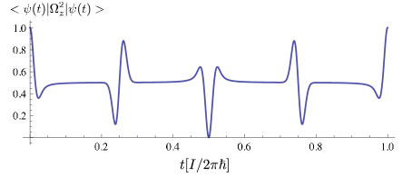
Figure 1: Collapse and revival of $\langle{\psi(t)}|\Omega_{z}^{2}|{\psi(t)}\rangle$ starting from a state localized about poles with width $\bar{\theta}=0.1$.

We now apply the rotor description to the quantum dynamics of antiferromagnetic condensates in the single mode regime, which is known to manifest rich behavior Romano and de Passos (2004); Diener and Ho ; Zhai et al. (2009). Here we consider preparing the system in the symmetry-broken nematic state given by Eq. (20), and then rapidly turning the magnetic field off and allowing the state to evolve freely. We note that according to the semiclassical theory (or by using the Gross-Pitaevskii equation) the nematic wavefunction will remain at the pole and not evolve temporally. The quantum mechanical dynamics, however, is markedly different. By dynamically evolving the wavefunction, Eq. (20), with the quantum rotor Hamiltonian Eq. (3) with $q=0$, it can be seen that the state will undergo periodic collapse and revival at the characteristic frequency $\hbar/I$. For instance, provided the initial state is sufficiently localized ${\bar{\theta}}\ll 1$, one can show that

$$\langle{\psi(t)}|\Omega_{z}^{2}|{\psi(t)}\rangle=2\bar{\theta}^{2}\sum_{{\rm odd}\;\ell>0}(2\ell+1)e^{-\ell(\ell+1)\bar{\theta}^{2}}\cos^{2}\left(\frac{(2\ell+1)\hbar t}{2I}\right).$$ (23)

The evolution of this function over a single period is plotted in Fig. 1. The localized nematic state rapidly collapses to states with substantial weight contributions from other regions of the unit sphere, and then fully revives at the end of the period. By applying the Poisson resummation formula to Eq. (23) it can be seen that the evolution is a train of localized pulses separated by a fourth of the time period. This behavior can be directly seen experimentally by measuring the time dependence of $\langle{a_{0}^{\dagger}a_{0}}\rangle$ after the turning off the magnetic used to prepare the system in the polar state. We note that since the magnetic field couples only to the spin degrees of freedom, the above procedure will not excite spatial modes of the condensate for sufficiently tight traps. The quantum collapse and revival of Fig. 1 is a direct consequence of the rotor mapping of spinor condensates.

In conclusion, we have established a correspondence between antiferromagnetic spinor condensates and quantum rotors. We have shown that this mapping offers a considerable conceptual as well as technical advance in understanding the properties of spinor condensates. We use the mapping to address recent experimental results Liu et al. (2009a, b) and to analytically predict a collapse and revival process (which is a direct experimental signature of quantum effects). We point out that it should be possible to provide similar quantum rotor mappings for condensates with larger spin.

We would like to acknowledge insightful discussions with S. Maxwell and P. Lett. This work was supported by JQI-NSF-PFC, DARPA QuEST, AFOSR, and ARO-DARPA-OLE.

References

- Liu et al. (2009a) Y. Liu, S. Jung, S. E. Maxwell, L. D. Turner, E. Tiesinga, and P. D. Lett, Phys. Rev. Lett. 102, 125301 (2009a).
- Liu et al. (2009b) Y. Liu, E. Gomez, S. E. Maxwell, L. D. Turner, E. Tiesinga, and P. D. Lett, Phys. Rev. Lett. 102, 225301 (2009b).
- Stenger et al. (1998) J. Stenger, S. Inouye, D. M. Stamper-Kurn, H. J. Miesner, A. P. Chikkatur, and W. Ketterle, Nature 396, 345 (1998).
- Chang et al. (2005) M. S. Chang, Q. S. Qin, W. X. Zhang, L. You, and M. S. Chapman, Nature Phys. 1, 111 (2005).
- Sadler et al. (2006) L. E. Sadler, J. M. Higbie, S. R. Leslie, M. Vengalattore, and D. M. Stamper-Kurn, Nature 443, 312 (2006).
- Klempt et al. (2009) C. Klempt, O. Topic, G. Gebreyesus, M. Scherer, T. Henninger, P. Hyllus, W. Ertmer, L. Santos, and J. J. Arlt, Phys. Rev. Lett. 103, 195302 (2009).
- (7) In terms of microscopic parameters, where is the mass of the constituent atoms, and are scattering lengths, and is the equilibrium density of the condensate.
- Law et al. (1998) C. K. Law, H. Pu, and N. P. Bigelow, Phys. Rev. Lett. 81, 5257 (1998).
- Ho (1998) T.-L. Ho, Phys. Rev. Lett. 81, 742 (1998).
- Ohmi and Machida (1998) T. Ohmi and K. Machida, J. Phys. Soc. Japan 67, 1822 (1998).
- Auerbach (New York, 1994) A. Auerbach, Interacting Electrons and Quantum Magnetism (Springer, New York, 1994).
- Anglin et al. (2001) J. R. Anglin, P. Drummond, and A. Smerzi, Phys. Rev. A 64, 063605 (2001).
- Ashhab and Leggett (2002) S. Ashhab and A. J. Leggett, Phys. Rev. A 65, 023604 (2002).
- Mueller et al. (2006) E. J. Mueller, T.-L. Ho, M. Ueda, and G. Baym, Phys. Rev. A 74, 033612 (2006).
- Zhou (2001) F. Zhou, Phys. Rev. Lett. 87, 080401 (2001).
- Demler and Zhou (2002) E. Demler and F. Zhou, Phys. Rev. Lett. 88, 163001 (2002).
- Imambekov et al. (2003) A. Imambekov, M. Lukin, and E. Demler, Phys. Rev. A 68, 063602 (2003).
- Cui et al. (2008) X. Cui, Y. Wang, and F. Zhou, Phys. Rev. A 78, 050701(R) (2008).
- Raghavan et al. (1999) S. Raghavan, A. Smerzi, S. Fantoni, and S. R. Shenoy, Phys. Rev. A 59, 620 (1999).
- Romano and de Passos (2004) D. R. Romano and E. J. V. de Passos, Phys. Rev. A 70, 043614 (2004).
- (21) R. Diener and T.-L. Ho, arXiv:cond-mat/0608732.
- Zhai et al. (2009) Q. Zhai, L. Chang, R. Lu, and L. You, Phys. Rev. A 79, 043608 (2009).