A near-infrared variability study in the cloud IC1396W: low star-forming efficiency and two new eclipsing binaries

Abstract

Identifying the population of young stellar objects (YSOs) in high extinction regions is a prerequisite for studies of star formation. This task is not trivial, as reddened background objects can be indistinguishable from YSOs in near-infrared colour-colour diagrams. Here we combine deep JHK photometry with J- and K-band lightcurves, obtained with UKIRT/WFCAM, to explore the YSO population in the dark cloud IC1396W. We demonstrate that a colour-variability criterion can provide useful constraints on the star forming activity in embedded regions. For IC1396W we find that a near-infrared colour analysis alone vastly overestimates the number of YSOs. In total, the globule probably harbours not more than ten YSOs, among them a system of two young stars embedded in a small ($\sim 10000$ AU) reflection nebula. This translates into a star forming efficiency SFE of $\sim 1$%, which is low compared with nearby more massive star forming regions, but similar to less massive globules. We confirm that IC1396W is likely associated with the IC1396 HII region. One possible explanation for the low SFE is the relatively large distance to the ionizing O-star in the central part of IC1396. Serendipitously, our variability campaign yields two new eclipsing binaries, and eight periodic variables, most of them with the characteristics of contact binaries.

1 Introduction

Our knowledge about the origin of low-mass stars is primarily based on observations of a few ($\sim 10$) nearby star forming regions. Although many of these regions are quite similar (for example, most of them do not harbour massive stars), there are indications for environmental differences in the outcome of star formation (e.g. Meyer et al., 2000; Slesnick et al., 2008; Luhman et al., 2009). Moreover, most of the extensively studied clouds are similar in star formation efficiency (Evans et al., 2009), indicating a comparable evolutionary state (see Forbrich et al., 2009, for an exceptional case) Hence, there is an incentive to extend our observational studies to more distant and diverse regions.

The problem is to find efficient means to identify clusters of embedded T Tauri stars. Since extinction is often too high for optical observations, the surveys are best carried out in the near/mid-infrared. The established method is to look for excess emission from circumstellar disks using colour-colour diagrams. At least in the near-infrared, however, reddenened background giants and extragalactic objects can occupy the same regions in colour-colour space as young stellar objects (YSOs), as extinction and disks can redden the colour in a similar way. Also, this method will only probe for classical T Tauri stars with disks (CTTS) and miss the population of diskless weak-line T Tauri stars (WTTS).

Thus, in order to select a more complete and less contaminated sample for follow-up spectroscopy, additional criteria have to be used to separate background/foreground objects from YSOs. One good option here is variability: T Tauri stars exhibit characteristic and well-studied photometric variations due to spots, activity, accretion, and disks (e.g. Herbst et al., 1994; Carpenter et al., 2001, 2002; Alves de Oliveira & Casali, 2008), which can easily be probed with relatively small telescopes. We present here a case study for a combined colour-variability criterion to identify YSOs in a high extinction region.

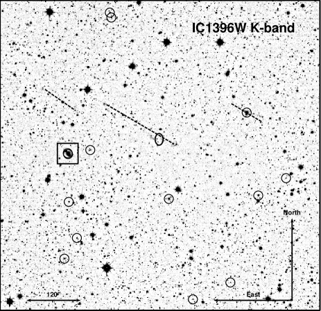
Figure 1: K-band image of the cloud IC1396W. This image has been created by co-adding the individual K-band frames from our time series observations. The positions and directions of the three outflows are indicated with dashed lines (Froebrich & Scholz, 2003). The position of IRAS 21246+5743 is marked with an ellipse. The YSO candidates identified in this paper (see Table 1) are marked with circles; one of them is further north and not seen in the image. The square indicates the position of the small nebula with two embedded YSOs, see Sect. 3.3 and Fig. 5.

Our target region is the dark cloud IC1396W in the vicinity, but outside, of the large HII region IC1396 which is ionized by the O6.5V star HD 206267. IC1396 contains several prominent examples of star forming activity, for example IC1396N (Codella et al., 2001; Nisini et al., 2001) and IC1396A (Reach et al., 2004), see Froebrich et al. (2005) for a summary. If IC1396W is associated with this region, the distance would be $\sim 750$ pc (Matthews, 1979), but so far no independent distance measurement is available. Given its relatively simple structure and radiation environment, the sample of globules in IC1396 is an ideal testbed to probe the effect of an ionizing star on the surrounding gas and embedded star forming activity. The available data is consistent with a scenario in which the radiation from the O star impacts both the globule masses and the star forming activity in the globules: With progressively larger distances from the ionizing star, the globule masses increase, while the star forming activity drops (Froebrich et al., 2005).

IC1396W contains the red source IRAS 21246+5743 and at least three molecular hydrogen outflows (Fig. 1, Froebrich & Scholz, 2003). Associated with these outflows are the features MHO 2267-2772 in the recently released Catalogue of Molecular Hydrogen Emission-Line Objects (Davis et al., 2010). Several of the H₂ emission features are detected in the optical as Herbig-Haro objects HH 864A-C by Froebrich et al. (2005). The same authors estimate the cloud mass to be about 500$\,M_{\odot}$ and the size to be $\sim 2$ pc, based on the distance of 750 pc, which makes it one of the largest clouds in the IC1396 region. The IRAS source seems to be a young Class-0 object of about 16$\,L_{\odot}$ and 33 K (Froebrich et al., 2003) and also the driving source of the main outflow HH864. The ISO maps at 160 and 200$\,\mu m$ give evidence for the presence of two more embedded sources close to the central object ($2.5^{\prime}$ SW and NE, respectively). Thus, this is a site of active, ongoing star formation.

In a shallow near-infrared survey, we found that IC1396W harbours a population of reddened objects, most of them clustered in a region coinciding with a clump of gas (Froebrich & Scholz, 2003). We present here new near-infrared observations to constrain the number and characteristics of young stars in this globule. The idea is to combine colours and variability in the near-infrared as indicator for youth. After discussing our observations and data reduction in Sect. 2, we search for YSOs in this region based on colour, variability, and complementary H$\alpha$ narrow band photometry in Sect. 3. As it turns out, IC1396W harbours only a small number ($\la 10$) of YSOs, indicating a low star formation efficiency (see Sect. 4). Our variability database yields a number of serendipitous discoveries, which are discussed in Sect. 5.

2 Data acquisition and analysis

2.1 Observations

We observed the cloud using the WFCAM instrument (Casali et al. 2007) at the UK Infra-Red Telescope. WFCAM houses 4 Rockwell Hawaii-II (HgCdTe 2048x2048) arrays spaced by 94% in the focal plane. A fixed optical auto-guider array is installed between these four arrays. The near-IR pixel size is 0$\aas@@fstack{\prime\prime}$4; consequently a single exposure covers 0.21 square degrees, with each chip covering $13.65^{\prime}\times 13.65^{\prime}$. WFCAM contains 8 filter paddles, one of which holds blanks for taking dark frames. We used the J- ($\lambda=1.25\,\mu m$, $\Delta\lambda=0.16\,\mu m$), H- ($\lambda=1.64\,\mu m$, $\Delta\lambda=0.29\,\mu m$), and K- ($\lambda=2.20\,\mu m$, $\Delta\lambda=0.34\,\mu m$) band filters. These filters meet the specifications of the Mauna Kea Consortium filter set (Tokunaga et al., 2002).

Time series observations alternately in the J- and K-band were obtained in the three nights 3-5 July 2006. In each of these three nights, the field was monitored over $\sim 5$ h. Additionally the field was observed in the H-band on July 2 2006. The seeing throughout these nights was mostly 0$\aas@@fstack{\prime\prime}$8-1$\aas@@fstack{\prime\prime}$1. In particular the first night (July 2) is affected by variable transparency due to cirrus.

The cloud IC1396W is small enough to fit into one WFCAM detector chip (see Fig. 1). We pointed detector 1 (the SW chip) to the target; the other three chips cover adjacent regions without evidence for star formation. A 5-point jitter was used in all observations. The detector was stepped in RA and DEC by integer multiples of 3$\aas@@fstack{\prime\prime}$2 or 6$\aas@@fstack{\prime\prime}$4. These steps represent an integer number of WFCAM IR array and autoguider CCD pixels. It also allows us to compensate for bad pixels. Additionally we used a ”2x2-small” microstep pattern with offsets of 1$\aas@@fstack{\prime\prime}$4. This results in proper sampling of the seeing with WFCAM’s 0$\aas@@fstack{\prime\prime}$4 pixels.

At each jitter position we integrated for $5\times 5$ sec. With the 20 positions (dithering and micro-stepping) we obtain an per pixel exposure time for each time series image of 500 sec in J- and K-band. There are 39 time series frames in J (13, 12, 14 in the three nights) and 38 in K (13, 11, 14). Additionally we obtained 8 images in the H-band with the same per pixel exposure time. Thus, for the co-added image of the region we have a per pixel integration time of 5.4 h in J, 1.1 h in H and 5.3 h in K.

To complement the near-infrared dataset, IC1396W was observed in the optical wavelength regime using the 2 m telescope of the Thüringer Landessternwarte Tautenburg (TLS) in its Schmidt mode. These observations were carried out with the 2k $\times$ 2k SITe CCD of $24\times 24\,\mu m$ pixel size, corresponding to a $42^{\prime}\times 42^{\prime}$ field of view, on December 7th 2007. The field was imaged in the R-band, a narrow-band filter centered on the H$\alpha$ emission line (6562 Å), and another narrow-band filter centered on 6673 Å. In the R band, three exposures were taken with an integration time of 100 sec each. The narrow band images were exposed 300 sec each. For calibration purposes domeflats and bias frames were included as well.

2.2 Image reduction and stacking

All WFCAM data were reduced by the Cambridge Astronomical Survey Unit (CASU) and are distributed through a dedicated archive hosted by the Wide Field Astronomy Unit (WFAU) in Edinburgh. The CASU reduction steps are described in detail by Dye et al. (2006); these include dark subtraction, bad pixel masking, flat fielding using twilight flats, and sky subtraction using a running average of frames obtained before and after each exposure. During this process the images are resampled to a scale of 0$\aas@@fstack{\prime\prime}$2/pixel. Astrometric and photometric calibrations are achieved using 2MASS point sources in each image (Dye et al., 2006; Hewett et al., 2006). We downloaded the fully-reduced images from WFAU. One reduced Multi-Extension Fits (MEF) file is available for each of the 39 (J), 38 (K) and 8 (H) time-series datasets; data from the four arrays in WFCAM are presented as separate images in each MEF.

To facilitate stacking and time series photometry, all images were co-centred using bright stars. The images were also cut so that only positions in the field covered in every individual image in the time series (J, H and K) are left. To obtain a deep image in each of the three bands we co-added the individual frames. Since the weather conditions were slighly variable, stars have a different signal-to-noise ratio in the images. Hence, each co-added frame was given a weight proportional to the ratio of flux divided by noise squared. This ensures that the resulting co-added image has the maximum signal to noise ratio (e.g. Froebrich & Meusinger, 2000). A coordinate system was matched to the stacked frame based on 2MASS objects in the field.

For the optical images from the TLS a standard reduction was carried out including the subtraction of an average bias frame as well as dividing by the normalized average flatfield.

2.3 Photometry and calibration

We produced a raw object catalogue based on the stacked K-band images for detector 1 (SW chip, the IC1396W field) and detector 4 (NW chip, $\sim 13^{\prime}$N of IC1396W, comparison field). This is done with the SExtractor software (Bertin & Arnouts, 1996) with default parameters. From this catalogue we rejected all objects with FWHM larger than 8 pixels and elongation $A/B>2$. This excludes a number of artefacts, barely resolved binaries, and galaxies. Still, the final catalogue does contain a significant fraction of extended objects.

The photometry for all time series images in J- and K-band as well as for the stacked images in JHK was carried out with the daophot-phot routine within IRAF. We kept a constant aperture of 10 pixels for all images. significantly larger than the typical seeing of 5 pixels. The sky background was estimated from a annulus with an inner radius of 15 pixels and 5 pixels width.

The photometry of the stacked frames was shifted to a standard system using $\sim 200$ bright stars in the field which are covered by 2MASS. We find zeropoints of 0.97, 1.19, and 0.60 mag for J-, H- and K-band, respectively. In addition, our photometry shows small colour terms with coefficients in the range of 0.03 mag in J- and H-band. We did not attempt an absolute calibration for the optical images.

For the time series photometry, a relative calibration is needed to account for the effects of variable transparency and variable seeing. This is done by deriving a reference lightcurve from a set of $\sim 150$ bright, non-variable stars for each field and filter, selected using the procedure outlined in Scholz & Eislöffel (2004). In short, from a large sample of several hundred lightcurves we selected the ones which show the minimum deviations from the ensemble lightcurve. These are averaged to define the reference lightcurve, which reflects the variations due to atmospheric effects. This reference lightcurve is subtracted from all lightcurves to correct for these effects.

3 Identifying young stellar objects

In the following section we will develop a strategy to find young stellar objects based on the combined information from near-infrared colours and variability. A few benefits and caveats of this method should be pointed out.

A colour criterion essentially probes for the presence of a hot, inner disk, which causes colour excess particularly in $H-K$. A selection based on near-infrared colour is expected to be strongly contaminated. As discussed for example in Robitaille et al. (2006), YSOs are expected to populate the area close or below the reddening band, and thus overlap in their colours with reddened background objects. A near-infrared colour selection is also incomplete as it misses objects without disks (weak-line T Tauri stars WTTS) or with inner disk holes.

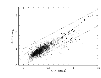
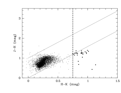
Figure 2: Colour-colour-diagram for the globule IC1396W (left panel) and a comparison field (right panel). For the colour criterium, we require the objects to have $H-K>0.75$. One datapoint at $H-K=1.9$ and $J-H=4.0$ is not plotted. The IC1396W field has 97 objects fulfilling the criterium. In the comparison field, 29 objects fulfill this limit, most of them are not point sources. The dotted lines show the reddening path over $A_{V}\sim 20$ mag (Mathis, 1990).

Variability in YSOs can be caused broadly by the presence of an accretion disk (hot spots or variable emission/absorption from the disk) and by magnetic activity (cool spots or flares). These processes will cause characteristic signatures in the near-infrared lightcurves (Alves de Oliveira & Casali, 2008; Scholz et al., 2009). As for the colour criterion, a YSO selection exclusively based on variability will be contaminated and incomplete. Based on the lightcurves it is not always possible to separate YSOs from field stars (e.g., magnetically active M dwarfs or short-period pulsating giants). This selection will miss YSOs without measurable variability, for example the ones without accretion and no detectable spot activity.

A combined colour-variability criterion can reliably establish a sample of YSOs with little contamination, but it will still not provide a complete census. Specifically it will miss 1) deeply embedded sources not visible in the near-infrared bands, 2) objects with small inner disk holes and thus no near-infrared excess, 3) WTTS without disk, 4) YSOs without measurable variability on the timescales of the observations. The first two groups can be identified with further photometric observations at longer wavelengths. WTTS can often be found based on variability alone, as they show periodic lightcurves on timescales of days and/or flare activity.

Group 4 may be of major relevance for our study, as our observations only cover three days: As discussed in Parihar et al. (2009), such relatively short runs might miss more than half of the variables in star forming regions. On timescales of several years, however, almost 100% of YSOs are found to be variable. This applies to variability amplitudes in the range of a few percent or larger, which is comparable to our detection limit. By combining our observations with 2MASS data we will look for missing objects with long-term variations (Sect. 3.4).

On the other hand, the fact that our run covers only a few nights helps us to rule out some classes of objects that are common contaminants in YSO surveys. For example, quasars may appear red, but their dominant variability modes have characteristic timescales in the order of years in the quasar rest frame, thus is unlikely to be found with the current dataset. The same argument applies to long-periodic pulsating red giants (e.g. Mira variables).

In summary, using colour or variability as observational indicators for youth gives incomplete and contaminated samples. Combining the two can potentially provide a much cleaner sample of YSO candidates, but will not completely solve the incompleteness issue.

3.1 The colour-colour diagram

From the calibrated photometry of the stacked images (see Sect. 2) a deep (H-K, J-H) colour-colour diagram was constructed, as commonly used to identify objects with disks. This was done for the field containing IC1396W in chip 1 as well as for the field covered by chip 4 for comparison. The full source catalogue for the IC1396W field has 8211 entries from which 7965 have reliable photometry in all three bands. Clearly the majority of these objects will not be young members of IC1396W.

A further cut was made by limiting the diagram to objects for which useful variability information is available. We include only sources for which the mean photometric noise, as determined from the lightcurves, is $<0.2$ mag in J- and K-band (see Sect. 3.2). This reduces the number of objects to 4397. The second cut imposes essentially a magnitude limit; while the full catalogue extends down to $J=22$ and $K=19.5$ mag, these values change to $J=19.4$ mag and $K=18.0$ mag after the variability information is taken into account. The comparison field has in total 7496 objects with photometry in all bands. After applying the variability cut a catalogue of 4422 objects is obtained, with limiting magnitudes of $J=19.3$ and $K=18.0$ mag.

The resulting colour-colour diagrams are shown in Fig. 2. The comparison field shows a clump of objects around (0.2,0.8) with a faint tail of objects with (small) $H-K$ excess. Most of the objects in this tail appear extended and may be red galaxies. There is no indication of strong extinction in the comparison field. The field around IC1396W shows the same clump of objects, but here it is stretched out along a well-defined path towards red colours. This is best explained by strong and variable extinction in the globule, which affects the colours from all background sources.

The dotted lines in Fig. 2 shows the standard interstellar reddening law with power law index $\beta=1.7$ (Mathis, 1990), which matches well with the vector of the reddening seen in this field. This provides reassurance in our colour calibration and shows that IC1396W does not exhibit an unusual $\beta$, as already shown by Froebrich & del Burgo (2006).

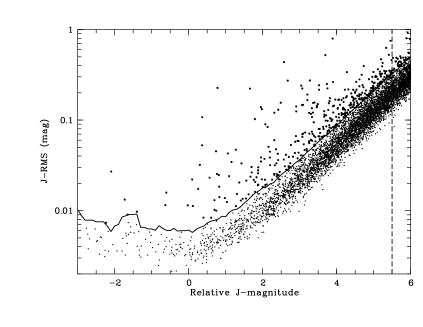
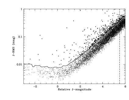
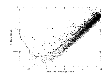
Figure 3: Variability diagram for the globule (left) and for the comparison field (right) in J (upper row) and K (lower row). All objects with RMS higher than the solid line are statistically variable ($F>2.6$) in comparison with the median RMS of stars with the same magnitude. The threshold is chosen to minimize the contamination. The zeropoint in relative magnitudes corresponds to $\sim 13.8$ in J-band and $\sim 12.8$ mag in K-band. Dashed lines mark the limit where the median RMS exceeds 0.2 mag

We use these diagrams to select a sample of objects with near-infrared colour excess, which could be considered candidates for classical T Tauri stars (CTTS). In the following these colour-selected objects will be called C-sample. CTTS usually occupy a region around or below the reddening vector, because they are affected by extinction and additional excess due to circumstellar emission (Meyer et al., 1997; Robitaille et al., 2006). We define a vertical colour cut (dashed line in Fig. 2) aiming to avoid the bulk of the population in the IC1396W area. The most reasonable results are achieved for $H-K>0.75$, which yields a C-sample of 97 objects for IC1396W and 29 for the comparison field. Shifting this boundary to the left by 0.1 almost doubles the number of objects in the IC1396W area, due to excessive contamination. The C-sample will be contaminated by the highly reddenened field stars, but also covers the typical colour range for CTTS.

3.2 Variability

In this section we select variable objects from our UKIRT dataset covering three observing nights. An object is considered variable if the photometric variations are significantly larger than the noise expected at this magnitude. This is tested by comparing the root mean square (RMS) with the median RMS for a given magnitude using a statistical test. The following steps are carried out for the J- and K-band data separately, in the IC1396W field and in the comparison field. The analysis starts with the database of lightcurves for all objects in the full source catalogue, i.e. 8211 for the IC1396W field.

In a first step we calculate the root mean square (RMS) from the lightcurves of all stars in the database. Three iterations of 3$\sigma$ clipping are carried out to exclude outliers. To quantify the photometric noise as a function of magnitude, we calculate a running median RMS for 0.5 mag wide bins and 0.1 mag stepsize from all lightcurves with at least 30 datapoints. This is based on the assumption that the overwhelming majority of the stars in our fields are non-variable for our photometric accuracy. Strictly speaking, we define ’variable’ relative to the bulk of field stars.

This yields an empirical function (see solid lines in Fig. 3), it reaches 5 mmag for bright, unsaturated stars and rises exponentially for fainter objects. The increase at the bright end can be attributed to the onset of non-linearity. A median RMS of 0.2 mag is reached at relative magnitudes of 5.5 in the J-band and 5.0 in K-band; objects with larger photometric noise are not considered. This cut-off is also used in the analysis of the colour-colour diagram (Sect. 3.1).

For any given star we then compare the actual RMS with the median RMS in the appropriate magnitude bin. We use the statistical F-test, which tests the zero hypothesis that the variances in two samples are consistent (where the variance is the square of the RMS). The test quantity $F$ is simply the ratio of measured variance vs. median variance; we are looking for lightcurves for which this quantity exceeds 1.0 significantly. For our lightcurves and assuming that the noise is Gaussian, $F\sim 2.2$ corresponds roughly to 1% likelihood that the zero hypothesis is valid, which is the false alarm probability for an object to be wrongly identified as variable at this F-level.

We choose a slightly higher threshold of $F=2.6$ to identify the sample of variables, aiming to reduce the contamination and to avoid the bulk of the datapoints. In Fig. 3 we show the RMS vs. magnitude diagram for J- and K-band. Overplotted in solid lines is the threshold for $F=2.6$. All objects above this threshold are marked. For the J-band this gives a sample of 389 out of 4800 objects with useful lightcurve. For K-band the variable sample has 320 out of 4878 objects. 165 objects are variable in both bands (called V-sample in the following).

The same procedure for the comparison field yields 417 variables in J-band, 286 in K-band, and 154 in both bands. The comparable number of variables in the two fields already indicates that IC1396W cannot harbour a large population of young, variable objects.

3.3 Combining colour and variability

In Fig. 4 we combine the information from the two previous subsections and look for overlap between C- and V-sample. The figures show the colour-colour diagrams for the IC1396W and the comparison field, as in Fig. 2. All objects from the V-sample are marked. The adopted threshold for the C-sample is shown as a dashed line.

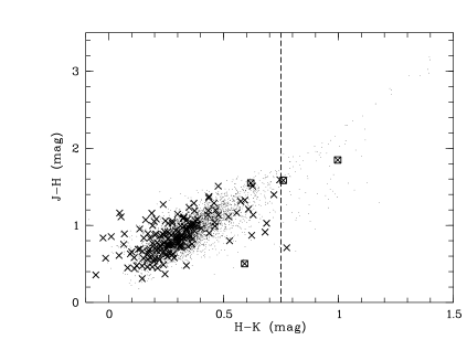
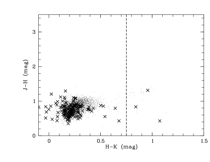
Figure 4: Colour-colour diagram for the globule (left panel) and the comparison field (right panel), variable objects are marked (crosses: variable in our time series, see Fig. 3; squares: variable in comparison with 2MASS data). The globule has 165 objects variable in K and J. In the comparison field, the same procedure gives 154 variable objects.

Quite obviously there is no significant population of objects in the globule which are reddened and variable. Most of the sources in the V-sample are scattered over the main bulk of datapoints at normal main-sequence colours. The number of red and variable objects is three in both fields. One of these sources in IC1396W is 12’ away from the globule core and thus likely contamination. The small overlap between red and variable objects argues for only a small population of YSOs in IC1396W.

Two of the sources in the C- and V-sample, 1-2189 and 1-2314, are located close together (2$\aas@@fstack{\prime\prime}$3), are unresolved in previous observations, and seen within a bright nebulosity, which has an entry in the 2MASS Extended Source Catalogue. It is located in a region of strong extinction, evidenced by low object density and red colours. This region has already been identified in Froebrich & Scholz (2003) as SE extension of the IC1396W cloud (see Fig. 1). All stars in the immediate neighbourhood of the nebula are significantly redder than our two candidates. The nebulosity is a fuzzy blob and does not show any resolved structure (apart from the point sources).

As shown in Fig. 5, the system actually harbours three point sources: The two red and variable objects, both with K-magnitudes of 11.3-11.5 mag and 2$\aas@@fstack{\prime\prime}$3 separated in NE-SW direction, plus a faint third object 1$\aas@@fstack{\prime\prime}$1 away from 1-2314, which is undetected in our catalogue. Another star (1-1996 with $K=12.6$) is seen to the NE just outside the nebula; with $H-K=1.4$ and $J-H=3.0$ this object is among the reddest in our catalogue with $A_{V}\sim 15-20$. It might be another embedded YSO or a background star.

The fact that 1-2189 and 1-2314 pass the colour-variability test combined with the characteristic of the nebula makes it likely that we are dealing with a system of young stellar objects embedded in a reflection nebula. Specifically, based on the location in a high-extinction area we argue that this is almost certainly not an extragalactic background object. If the distance of 750 pc for IC1396W is correct (see Sect. 4.2), the separation for the two stars in the nebulosity is 1700 AU in projection, the diameter of the nebulosity $\sim 10000$ AU. Thus, this looks like a typical localized cell of star formation as they are commonly found for example in the Taurus-Auriga star forming region.

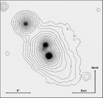
Figure 5: K-band image of two red and variable objects in a nebula, N is up and E is left. The objects 1-2314 and 1-2189 are seen in the center, together with a faint third source. The object 1-1996 is seen towards the NE. Contours are on a log-scale from 10 to 10000 counts.

3.4 Probing long-term variability

As mentioned earlier, the concern is that our relatively short monitoring run does not allow us to identify objects that are variable on long timescales. The 2MASS data is used to check for long-term variability for the brighter objects in our catalogue. We find 595 counterparts with photometry in the 2MASS database, taken several years earlier than our own data. This implies that the test can only be carried out for 14% of the total sample considered in the previous sections. In addition, our information about long-term variability is limited because 2MASS provides only one epoch. Hence, we might miss long-term variables, particularly at the faint end of our survey.

For the overwhelming majority of the objects with 2MASS counterpart the difference between our magnitudes and the 2MASS values is within the expected photometric errors. For example, the deviations in the J-band are $<0.1$ mag down to $J=15$ mag. Five objects were found with clear discrepancy between 2MASS and our magnitude in J- and K-band. However, all five are already contained in our V-sample for J- as well as K-band, i.e. this test does not yield any new candidates and confirms the scarcity of YSOs in IC1396W. In Fig. 4 these five objects are shown with squares. This includes the red sources identified in the nebulosity (see Sect. 3.3); in these cases however the test is unreliable, as they are not resolved in 2MASS. The total near-infrared brightness in the Extended Source Catalogue is comparable to the combined flux from the two point sources.

3.5 Variability characteristics

On the timescales covered by our time series, young stellar objects frequently show two types of variability: a) strictly periodic with amplitudes $\la 0.2$ mag, b) partly irregular variations with large amplitudes often exceeding 0.5 mag. These two categories represent the type I and type II variability identified by Herbst et al. (1994). While type I is caused by magnetically induced cool spots corotating with the objects, type II is related to the accretion flow and can contain periodic components, irregular eclipses, and burst-like phenomena. In addition, young stars can show chromospheric flare events, but we expect this to be rare in the near-infrared.

Type II variations are easily spotted by visual inspection of the lightcurves (see example lightcurves in Scholz & Eislöffel, 2005). We examined the lightcurves of variable objects in the globule area carefully. This was restricted to the objects within $<9^{\prime}$ distance from IRAS 21246+5743. Out of 165 objects 89 fulfill this criterion. Nine of them show well-defined variations after visual inspection, including two obvious and regular eclipses (1-2750, 1-3677), discussed in Sect. 5. None has the characteristic type II variations discussed above.

In this sample of 89 objects we searched for periodicities. In most cases the variability in YSOs is more pronounced in the J- than in the K-band (Carpenter et al., 2001); therefore the period search is based on the J-band lightcurves. Taking into account our limited sample of $<40$ datapoints per lightcurve, we refrain from using periodogram analysis, instead we have chosen a robust and simple approach: For a set of periods ranging from 0.0 to 2.5 d in steps of 0.015 d, a given lightcurve was fit with a sine function. After subtraction of the best-fitting sinecurve, our routine compares the variance in the original lightcurve with the variance in the residuals using the F-test (see Sect. 3.2). This essentially probes how much of the variability in the lightcurve can be attributed to a sinusoidal period.

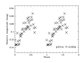
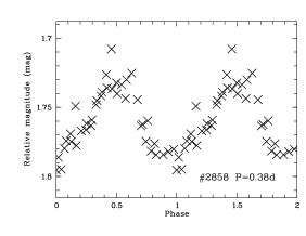
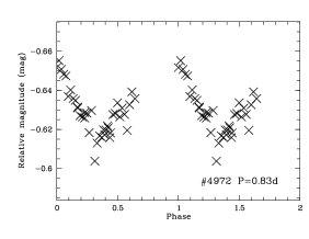
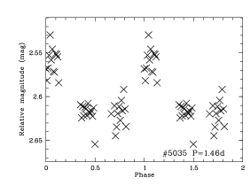
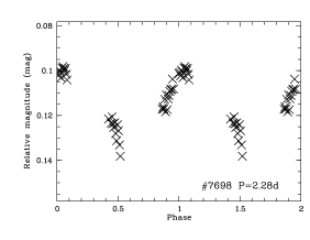
Figure 6: J-band lightcurves for the stars with significant periodic variations plotted as function of phase. Object ids refer to the catalogue for chip 1.

Out of 89, 11 lightcurves exhibit a periodic signal with $F>2.5$, including the two eclipses. Five objects have clearly pronounced variations with periods ranging from 0.4 to 2.3 d. One of these objects the only one which fulfills the colour criterion in Sect. 3.1, is 1-2314, located in the bright nebulosity discussed in Sect. 3.3. We note that the second red and variable object in this nebula (1-2189) shows a steady decline of 0.15 mag over the three observing nights, possible due to a longer period. The best five periods are shown in Fig. 6 (1-2314, 1-2858, 1-4972, 1-5035, 1-7698). All these periodicities have amplitudes $<0.1$ mag. Amplitudes and periods are typical for rotational modulations in young stars, caused by cool spots.

One more (1-6059) has a period of 0.25 d and a large amplitude of 0.4 mag. It has a J-band magnitude of 16.6, which would put it in the substellar regime, if it is a member of IC1396W, but the colour $H-K=0.2$ is not matching. It is also relatively far away from the core of the globule (8’). This strongly argues against membership. This object is further discussed in Sect. 5.

3.6 H$\alpha$ photometry

We use the optical photometry in the filter centered on the H$\alpha$ emission line as additional check for young stellar objects in IC1396W. The optical catalogue contains 11357 objects with good photometry in all bands, from which 533 are within a 9’ radius of the globule center. Fig. 7 shows the H$\alpha$ ’colour’ (i.e. the difference in instrumental magnitudes between the flux in H$\alpha$ and the flux in a filter next to the H$\alpha$ feature) vs. R-band magnitude for these 533 objects. About 70% of them have a counterpart in the near-infrared catalogue.

For clusters with a strong YSO population this type of diagram is expected to show a bimodal population (main-sequence and YSO), as for example seen in Lamm et al. (2004). Our plot does not show any sign of bimodality, again indicating that IC1396W does not harbour a significant number of YSOs. The datapoints form a symmetric distribution around $H_{a}-H_{av}=0.05$ which is likely the locus of the background main-sequence. The scatter of the datapoints at the faint end of the plot is consistent with the photometric uncertainty.

Objects with strong H$\alpha$ emission are expected to be located below this line. Only three objects fall below the line on a confidence level much better than 3$\sigma$. Two of them are clearly identified in the K-band image as part of the SW head of the largest outflow in the cloud, which is visible in the optical bands as well. 1-2223 has a point-source counterpart in the near-infrared, which is neither variable nor red; this might be a disk-less WTTS. A handful of additional objects is close to the 3$\sigma$ limit; we do not consider them to be good candidates due to the lack of separation in H$\alpha$ colour between them and the bulk of the datapoints.

Overplotted in Fig. 7 are red objects (plusses) according to our $H-K$ criterion on Sect. 3.1 (only object 1-2314, as most red sources are not detected in the optical), variable objects (crosses) in J- and K-band according to the criterion in Sect. 3.2, which includes four objects with significant periods (Sect. 3.5) shown with triangles.

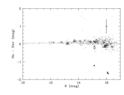
Figure 7: H$\alpha$ ’colour’ vs. R-band magnitude for the IC1396W field, derived from the complementary optical observations. The filled squares mark objects with clear H$\alpha$ emission. Objects with $H-K$ colour excess are marked with plusses, variable objects with crosses, and objects with significant periods with triangles. The errorbarat $R=16$ mag corresponds to the 3$\sigma$ uncertainty.

4 Star formation in IC1396W

4.1 The YSO census

Based on the discussion in Sect. 3 we will compile samples of candidate YSOs in the IC1396W globule. We distinguish five groups of objects. For all five groups we additionally require the objects to be point sources and to be spatially located within the area of the globule ($<9^{\prime}$ distance from IRAS 21246+5743):

1. $H-K$ excess and variability: Only two objects fulfill these criteria, with $K=11.3$ and $K=11.5$ (1-2189 and 1-2314). As mentioned in Sect. 3.3, both are located close together in a bright nebulosity.

2. $H-K$ excess and located on the axis of one of the three outflows, classifying them as possible outflow driving sources: One source with $K=10.7$ (1-5864) falls on the axis for the northwestern outflow. This objects has already been discussed in Froebrich & Scholz (2003) as a possible driving source for this outflow.

3. $H-K$ excess and located below the reddening path in the colour-colour diagram: From our C-sample, 78 objects are in the globule area, from which 54 look like point sources. 7 of these objects are located significantly below the well-defined reddening path of the remaining objects, with K-band magnitudes between 15.0 and 16.5. This sample likely contains reddenened background objects.

4. Variability characteristic typical for YSOs: From our V-sample, 89 objects are in the globule area, and four of them show YSO-like variability (see Sect. 3.5), with K-band magnitudes between 12.1 and 15.3. This sample likely contains variable field objects (e.g. active M dwarfs or short-period pulsating giants).

5. H$\alpha$ emission detected using our photometric criterion as defined in Sect. 3.6: Only one object, 1-2223, fulfills this criterion, it has a K-band magnitude of 13.8.

In Table 1 we list the coordinates and photometry for the candidates selected based on these four criteria; their positions are overplotted in Fig. 1. In total, 15 candidates are identified from colour, variability, and spatial position. All require spectroscopic confirmation, in particular the groups (iii)-(v). Five of them do not show colour excess and could thus be WTTS in IC1396W. In addition, the globule is known to harbour the likely Class 0 source IRAS 21246+5743 (Froebrich et al., 2003). This can be contrasted with the 31 red objects identified in the shallow survey by Froebrich & Scholz (2003). A pure colour selection, as used by Froebrich & Scholz (2003), clearly overestimates the number of YSOs in the cloud.

The depth and completeness of our sample is not trivial to determine, because we used a variety of different indicators. Our photometry database requires the objects to have uncertainties $<0.2$ mag in K- and J-band, which effectively limits the survey to $J<19$ mag (Sect. 3.1). Assuming a maximum extinction of $A_{V}=10$ mag and a distance of 750 pc, this corresponds to $M_{J}\sim 7$. With the 1 Myr track by Baraffe et al. (1998) this yields a mass limit $\sim 0.05\,M_{\odot}$, which is applicable to categories (i), (ii) and (iii) above. Since all objects identified in category (iv) have amplitudes $<0.1$ mag, the depth for this sample is likely to be 2-3 mag lower, corresponding to $\sim 0.2\,M_{\odot}$. Thus, the survey covers the regime around the peak in the IMF.

The sample of candidate YSOs in the categories (iii)-(v) may contain a substantial fraction of contaminating background objects. On the other hand our method will miss certain types of sources (see discussion in 3). It is sensitive to CTTS and variable WTTS, which are the major fractions of objects in regions at 1 Myr. Therefore we do not expect that the incompleteness affects our most relevant result: The number of candidate YSOs in this globule is found to be low, probably less than 10.

Table 1: Candidate YSOs in IC1396W. The five groups of objects in this table correspond to the groups (i)-(v) described in the text (Sect. 4.1).

ID	$\alpha$ (J2000)	$\delta$ (J2000)	$K$ (mag)	$H-K$	$J-H$
1-2189	21:26:31.44	57:55:50.90	11.29	1.00	1.85
1-2314	21:26:31.53	57:55:52.80	11.51	0.76	1.58
1-5864	21:25:41.63	57:57:18.6	10.68	1.40	3.15
1-2368	21:26:31.30	57:54:05.2	15.53	0.77	1.26
1-2560	21:26:29.12	57:52:45.1	15.75	1.18	1.30
1-3314	21:26:19.58	58:01:02.6	15.80	0.79	1.44
1-3366	21:26:19.16	58:00:51.7	16.14	0.89	1.64
1-4467	21:26:03.49	57:54:09.6	14.96	0.97	1.60
1-5828	21:25:46.53	57:51:02.7	16.48	0.99	0.95
1-7003	21:25:30.81	57:54:52.2	16.50	1.07	1.46
1-2858	21:26:25.26	57:55:59.5	14.40	0.24	0.87
1-4972	21:25:56.16	58:02:16.9	12.11	0.27	0.74
1-5035	21:25:56.98	57:50:26.3	15.33	0.24	0.77
1-7698	21:25:38.58	57:54:14.6	13.08	0.18	0.59
1-2223	21 26 31.57	57 55 52.6	13.84	0.25	0.82

¹ possible source for outflow 3, see Froebrich & Scholz (2003)

4.2 Star formation efficiency

IC1396W is one of the largest and most massive clouds in the IC1396 region. Froebrich et al. (2005) determined a globule mass of 400-550$\,M_{\odot}$ from near-infrared extinction maps, assuming a distance of 750 pc. Combined with the low number of YSOs this indicates low star formation efficiency. Before we can quantify this more accurately, however, we re-assess the distance of IC1396W.

A standard way of probing distances to dense clouds is by separating foreground and background objects using the near-infrared colour and comparing the number of foreground objects with predictions from stellar population models. In IC1396W this procedure is only applicable to the innermost part of the cloud, where the extinction is strong enough to block the background objects. Within 1.5’ from the IRAS source there are 8 objects with unreddened colours of $J-K\sim 1.0$, which agrees well with the typical colours of objects outside the cloud. The other 14 objects in this area are clearly reddened with $J-K>1.5$.

We used the Galaxy model from the Besancon group to simulate a catalogue of objects over an area of 1 sqdeg in the direction of IC1396W matching the dynamic range of our catalogue ($9.3<K<18.7$ mag). This yields 4798 objects with distance $<750$ pc, which corresponds to 9 objects for an area of $\pi R^{2}$ with $R=1.5^{\prime}$. Thus, the model predicts a number of foreground objects that is remarkably close to the actual number of foreground objects. This indicates that the assumption of $d=750$ pc is plausible. Assuming Poissonian errors, the distance is unlikely to be below $d=600$ pc.

Thus the estimates for the cloud mass reported above are valid. As discussed in Sect. 4.1 the number of YSOs in IC1396W is likely to be around 10 or less. Assuming an average mass of $\sim 0.5\,M_{\odot}$ gives a total stellar mass of 5$\,M_{\odot}$ and a star forming efficiency SFE around 1%. This can be compared with SFE values determined for nearby star forming regions: According to Evans et al. (2009) star formation is significantly more efficient ($\geq 3$%) in Cha II, Lupus, Perseus, Serpens, and Ophiuchus. With the exception of Cha II, these clouds are much more massive than IC1396W. On the other hand, IC1396W is comparable in SFE with cores without stellar clusters in Cepheus (Kirk et al., 2009), but exceeds all these regions in mass. Thus, our survey establishes IC1396W as an intermediate case of a relatively massive cloud with low star formation efficiency. The SFE is still about one order of magnitude higher than in the Pipe nebula (0.06%, Forbrich et al., 2009), which appears to be a cloud in the earliest phases of star formation.

There are indications that the radiation from the O6.5V star in the center of the HII region IC1396 has an impact on the star forming activity in the surrounding clouds (Froebrich et al., 2005), i.e. clouds at larger distances are bigger and less active. IC1396W is one of the more remote clouds in this region, the distance from the exciting bright star is around 25 pc. This could explain why the star forming efficiency in IC1396W is found to be low.

5 Serendipitous discoveries

While visually inspecting the lightcurves, we noticed a number of obvious variable objects. In the following we report on the most prominent examples, including two eclipsing binaries and 8 periodic variables. All these objects fulfill the conditions for variable objects as outlined in Sect. 3.2. For the eclipsing binaries we present additional low-resolution spectra. Further analysis of these serendipitously discovered objects is postponed for future studies.

5.1 Eclipsing binaries

In the field of IC1396W there are two stars which show clear, deep eclipses in our lightcurves. In both cases we observe only one eclipse, i.e. we cannot constrain the period. Based on the symmetry of the ellipses and the smooth ingress/egress, we interpret the sources as eclipsing binaries, although in principle other origins are conceivable (e.g., eclipses by circumstellar material). The parameters of these systems are given in Table 2, their lightcurves are plotted in Fig. 8.

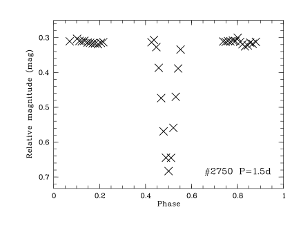
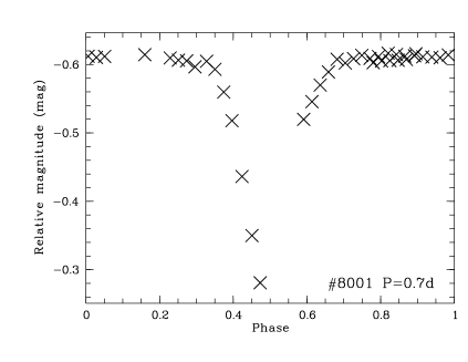
Figure 8: Eclipses found in our lightcurves, J-band datapoints plotted as function of phase. The periods are not constrained by our lightcurves; shown are examplarily fits. Object ids refer to the catalogue for chip 1.

Table 2: Eclipsing binaries in our monitoring field.

ID	$\alpha$ (J2000)	$\delta$ (J2000)	$K$ (mag)	$H-K$	$J-H$	$\Delta J$	$\Delta K$
1-2750	21:26:25.71	57:59:02.4	12.85	0.35	0.84	0.38	0.37
1-8001	21:25:23.40	57:49:35.5	12.42	0.24	0.49	$>0.06$	$>0.07$

If these eclipsing binaries are associated with the young population of IC1396W, they are of particular interest to constrain the fundamental properties of young low-mass objects. This motivated us to obtain follow-up spectra to look for evidence of youth. The ISIS spectrograph at the William Herschel Telescope was used to observe these objects with grisms R158R (1.8 Å per pixel, 30 min integration time, date 18/07/2008) and R1200R (0.26 Å per pixel, 30 min, 21/07/2007 and 13/10/2008). All data was taken in Service Mode. A spectroscopic standard reduction was carried out for these spectra, including bias and flatfield correction and background removal by subtracting a onedimensional fit along the spatial direction. The spectra are exctracted using apall within IRAF. Wavelength calibration is done based on Cu-Ar arc spectra. The low-resolution data is flux calibrated based on a spectrum for the standard star SP2157+261. The results are shown in Fig. 9.

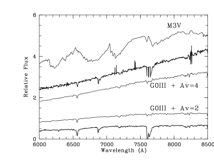
Figure 9: Low-resolution spectra for the two eclipsing binaries near the cloud IC1396W. The thick solid lines are the spectra for 1-2750 (upper) and 1-8001 (lower). The thin lines show template spectra for a reddened G0III giant and a M3V dwarf from Pickles (1998). The absorption features at 6850 and 7600 Å are telluric bands. The spikes at 7100 and 7400 Å in the spectrum of 1-2750 are caused by cosmics.

Based on the spectra it is safe to say that the eclipsing binaries are not associated with the young population in IC1396W. Three arguments are important here: a) There is no evidence for H$\alpha$ emission typical for YSOs, either due to accretion or magnetic activity. In fact, H$\alpha$ is observed as an unshifted absorption line which also excludes the interpretation as extragalactic objects. b) The high-resolution spectra, albeit at low signal-to-noise ratio, do not show any evidence for the deep Lithium absorption feature at 6709Å which is found in young stars with equivalent widths of $\sim 0.5$ Å (Mentuch et al., 2008). c) If the objects are at the distance of IC1396W and have an age of 1 Myr they are expected to be M-type stars (Luhman et al., 2003), which is inconsistent with the spectra (see Fig. 9). In particular, the characteristic TiO bandhead at 7050 Å and the CaH absorption at 6830 Å are absent and the slope is almost flat.

Additionally, the two objects are $>5^{\prime}$ away from the IRAS source in the core of the cloud. Their colours indicate little reddening and there is no significant colour variability. All this argues against association with IC1396W. We conclude that these are objects in the background of the cloud.

The spectra are well-approximated with F- or G-type templates with little reddening, as seen in Fig. 9. This is also consistent with the near-infrared colours: For a G0-type star (luminosity class III or V) the intrinsic $H-K$ is 0.05 (Bessell & Brett, 1988), which yields $H-K=0.2$ for $A_{V}=2$ (E-2) and 0.35 for $A_{V}=4$ mag (E-1). The same testcase gives $J-H=0.6$ for $A_{V}=2$ and 0.85 for $A_{V}=4$. All this is in perfect agreement with our measurements.

From the colours and the low-resolution spectra we cannot definitely tell if these two are giants or dwarfs. For a G0 dwarf the K-band flux would indicate a distance of $\sim 1$ kpc, for a giant about 5 kpc. The sharpness of the eclipses favours dwarfs, as a giant is more likely to produce a slow ingress and egress. Another argument for dwarfs is the relatively low extinction. (With $A_{V}\sim 0.7$ mag/kpc we would expect $H_{K}>0.5$ for giants.)

The lack of a flat phase in eclipse, the depth of the eclipses, and the lack of colour change in eclipse argues for systems with roughly equal size components. Due to their faintness we did not attempt to obtain radial velocity monitoring to constrain their fundamental parameters. Anybody interested in working on these objects is encouraged to get in touch with us.

5.2 Periodic variables

In our database for the IC1396W field and the comparison field we noticed 9 obvious short-period variables with large amplitudes (see Table 3). The periods for these objects were estimated using the procedure outlined in Sect. 3.5. They all have periods ranging from 0.1 to 0.4 d and J-band amplitudes from 0.1 to 0.6 mag. We show their lightcurves plotted in phase to the period in Fig. 10. Most of the lightcurves show evidence for changes in the brightness of maxima and minima on timescales of a few cycles, which is best explained by multiple periodicities being superimposed in the lightcurve.

Lacking spectra it is difficult to definitely determine the nature of these objects. Most of them are good candidates for contact binaries. The CB frequency relative to field stars has been determined to $1/500$ for $M_{V}>+1.5$ (Rucinski, 2002). Both fields combined we have monitored $\sim 7000$ stars for which variations of $\ga 0.1$ mag are easily detectable, i.e. we could expect up to $\sim 14$ W UMa stars among them, which is an upper limit, since our database is expected to include a significant fraction of giants.

Table 3: Periodic variables in our monitoring field. Amplitudes measured from the first observing night.

ID	$\alpha$ (J2000)	$\delta$ (J2000)	$K$ (mag)	$H-K$	$J-H$	$\Delta$J	$\Delta K$	P (d)	Comments
1-1141	21:26:45.43	57:59:42.3	13.86	0.24	0.92	0.13	0.12	0.436	max/min change
1-6059	21:25:43.09	57:50:48:7	15.91	0.20	0.53	0.42	0.35	0.253	max/min change
1-6221	21:25:21.26	57:49:58:8	15.16	0.22	0.73	0.34	0.35	0.129	max/min change
4-1008	21:26:57.27	58:17:42.5	13.69	0.16	0.52	0.08	0.07	0.433	max/min change
4-2728	21:25:46.49	58:20:36.7	15.81	0.13	0.82	0.60	0.46	0.249	max/min change
4-4066	21:26:44.37	58:23:19.2	11.55	0.18	0.54	0.28	0.27	0.241	eclipse?
4-5549	21:25:35.93	58:25:39.2	16.89	0.30	0.52	0.38	0.48	0.213	max/min change
4-5676	21:26:23.18	58:26:10.9	11.58	0.28	0.49	0.28	0.25	0.311

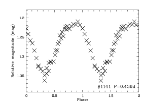
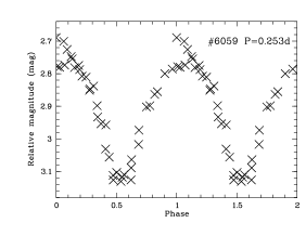
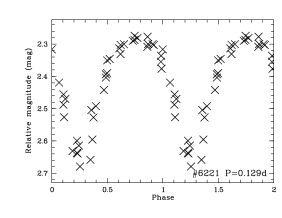
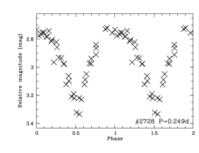
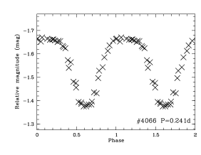
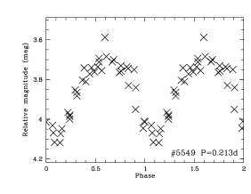
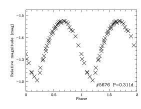
Figure 10: Periodic variables found in our lightcurves, J-band datapoints plotted as function of phase. Object ids refer to the catalogue for chip 1 for the 1st row of panels, to the catalogue for chip 4 for the 2nd and 3rd row.

The brighter ones could also be pulsating RR Lyr stars at distances of $>2$ kpc. For the fainter objects, this would imply unrealistically large distances. Some of the periodic stars could be $\delta$ Scuti pulsating variables, particularly the ones with relatively low amplitudes. The sample may also include spotted, rotating variables (BY Draconis or FK Comae type); 1-1141 and 4-1008 might be candidates for these types of stars. However, the short periods, large amplitudes, and min/max changes are atypical for spotted stars. Finally, 4-4066 could alternatively be a detached or semi-detached eclipsing binary.

References

- Alves de Oliveira & Casali (2008) Alves de Oliveira C., Casali M., 2008, A&A, 485, 155
- Baraffe et al. (1998) Baraffe I., Chabrier G., Allard F., Hauschildt P. H., 1998, A&A, 337, 403
- Bertin & Arnouts (1996) Bertin E., Arnouts S., 1996, A&AS, 117, 393
- Bessell & Brett (1988) Bessell M. S., Brett J. M., 1988, PASP, 100, 1134
- Carpenter et al. (2001) Carpenter J. M., Hillenbrand L. A., Skrutskie M. F., 2001, AJ, 121, 3160
- Carpenter et al. (2002) Carpenter J. M., Hillenbrand L. A., Skrutskie M. F., Meyer M. R., 2002, AJ, 124, 1001
- Codella et al. (2001) Codella C., Bachiller R., Nisini B., Saraceno P., Testi L., 2001, A&A, 376, 271
- Davis et al. (2010) Davis C. J., Gell R., Khanzadyan T., Smith M. D., Jenness T., 2010, A&A, 511, A24+
- Dye et al. (2006) Dye S., Warren S. J., Hambly N. C., Cross N. J. G., Hodgkin S. T., Irwin M. J., Lawrence A., Adamson A. J., Almaini O., Edge A. C., Hirst P., Jameson R. F., Lucas P. W., van Breukelen C., Bryant J., Casali M., Collins R. S., Dalton G. B., Davies J. I., Davis C. J., Emerson J. P., Evans D. W., Foucaud S., Gonzales-Solares E. A., Hewett P. C., Kendall T. R., Kerr T. H., Leggett S. K., Lodieu N., Loveday J., Lewis J. R., Mann R. G., McMahon R. G., Mortlock D. J., Nakajima Y., Pinfield D. J., Rawlings M. G., Read M. A., Riello M., Sekiguchi K., Smith A. J., Sutorius E. T. W., Varricatt W., Walton N. A., Weatherley S. J., 2006, MNRAS, 372, 1227
- Evans et al. (2009) Evans N. J., Dunham M. M., Jørgensen J. K., Enoch M. L., Merín B., van Dishoeck E. F., Alcalá J. M., Myers P. C., Stapelfeldt K. R., Huard T. L., Allen L. E., Harvey P. M., van Kempen T., Blake G. A., Koerner D. W., Mundy L. G., Padgett D. L., Sargent A. I., 2009, ApJS, 181, 321
- Forbrich et al. (2009) Forbrich J., Lada C. J., Muench A. A., Alves J., Lombardi M., 2009, ApJ, 704, 292
- Froebrich & del Burgo (2006) Froebrich D., del Burgo C., 2006, MNRAS, 369, 1901
- Froebrich & Meusinger (2000) Froebrich D., Meusinger H., 2000, A&AS, 145, 229
- Froebrich & Scholz (2003) Froebrich D., Scholz A., 2003, A&A, 407, 207
- Froebrich et al. (2005) Froebrich D., Scholz A., Eislöffel J., Murphy G. C., 2005, A&A, 432, 575
- Froebrich et al. (2003) Froebrich D., Smith M. D., Hodapp K., Eislöffel J., 2003, MNRAS, 346, 163
- Herbst et al. (1994) Herbst W., Herbst D. K., Grossman E. J., Weinstein D., 1994, AJ, 108, 1906
- Hewett et al. (2006) Hewett P. C., Warren S. J., Leggett S. K., Hodgkin S. T., 2006, MNRAS, 367, 454
- Kirk et al. (2009) Kirk J. M., Ward-Thompson D., Di Francesco J., Bourke T. L., Evans N. J., Merín B., Allen L. E., Cieza L. A., Dunham M. M., Harvey P., Huard T., Jørgensen J. K., Miller J. F., Noriega-Crespo A., Peterson D., Ray T. P., Rebull L. M., 2009, ApJS, 185, 198
- Lamm et al. (2004) Lamm M. H., Bailer-Jones C. A. L., Mundt R., Herbst W., Scholz A., 2004, A&A, 417, 557
- Luhman et al. (2009) Luhman K. L., Mamajek E. E., Allen P. R., Cruz K. L., 2009, ApJ, 703, 399
- Luhman et al. (2003) Luhman K. L., Stauffer J. R., Muench A. A., Rieke G. H., Lada E. A., Bouvier J., Lada C. J., 2003, ApJ, 593, 1093
- Mathis (1990) Mathis J. S., 1990, ARA&A, 28, 37
- Matthews (1979) Matthews H. I., 1979, A&A, 75, 345
- Mentuch et al. (2008) Mentuch E., Brandeker A., van Kerkwijk M. H., Jayawardhana R., Hauschildt P. H., 2008, ApJ, 689, 1127
- Meyer et al. (2000) Meyer M. R., Adams F. C., Hillenbrand L. A., Carpenter J. M., Larson R. B., 2000, Protostars and Planets IV, 121
- Meyer et al. (1997) Meyer M. R., Calvet N., Hillenbrand L. A., 1997, AJ, 114, 288
- Nisini et al. (2001) Nisini B., Massi F., Vitali F., Giannini T., Lorenzetti D., Di Paola A., Codella C., D’Alessio F., Speziali R., 2001, A&A, 376, 553
- Parihar et al. (2009) Parihar P., Messina S., Distefano E., Shantikumar N. S., Medhi B. J., 2009, MNRAS, 400, 603
- Pickles (1998) Pickles A. J., 1998, PASP, 110, 863
- Reach et al. (2004) Reach W. T., Rho J., Young E., Muzerolle J., Fajardo-Acosta S., Hartmann L., Sicilia-Aguilar A., Allen L., Carey S., Cuillandre J., Jarrett T. H., Lowrance P., Marston A., Noriega-Crespo A., Hurt R. L., 2004, ApJS, 154, 385
- Robitaille et al. (2006) Robitaille T. P., Whitney B. A., Indebetouw R., Wood K., Denzmore P., 2006, ApJS, 167, 256
- Rucinski (2002) Rucinski S. M., 2002, PASP, 114, 1124
- Scholz & Eislöffel (2004) Scholz A., Eislöffel J., 2004, A&A, 419, 249
- Scholz & Eislöffel (2005) —, 2005, A&A, 429, 1007
- Scholz et al. (2009) Scholz A., Xu X., Jayawardhana R., Wood K., Eislöffel J., Quinn C., 2009, MNRAS, 398, 873
- Slesnick et al. (2008) Slesnick C. L., Hillenbrand L. A., Carpenter J. M., 2008, ApJ, 688, 377
- Tokunaga et al. (2002) Tokunaga A. T., Simons D. A., Vacca W. D., 2002, PASP, 114, 180
- Zhou et al. (2006) Zhou J., Zhang X., Zhang H., Esimbek J., Zhang J., Ju B., 2006, New Astronomy, 12, 111