$D^{*}D\rho$ vertex from QCD sum rules

Abstract

We calculate the form factors and the coupling constant in the $D^{*}D\rho$ vertex in the framework of QCD sum rules. We evaluate the three point correlation functions of the vertex considering both $D$ and $\rho$ mesons off–shell. The form factors obtained are very different but give the same coupling constant: $g_{D^{*}D\rho}=4.1\pm 0.1$ GeV^-1.

I Introduction

Over the last years the strong interaction of charmed hadrons among themselves and with other species of hadrons has received increasing attention. From the discovery of charmed mesons in the seventies until the late eighties there was no motivation to study in detail the interactions of these particles. In the early nineties there was a series of papers trying to compute the cross section of a $J/\psi$ with ordinary light hadrons. The motivation came from the heavy ion program running at CERN and later at RHIC. At that time $J/\psi$ suppression was considered as a signature of quark gluon plasma (QGP) formation and it was very important to know as accurately as possible the purely hadronic (non-QGP induced) charmonium suppression, which would be the background for the QGP signal. From 2000 on, it became slowly clear that the physics of $J/\psi$ is much more complex than thought before and its simple suppression was no longer considered as a QGP signal and the subject lost interest. On the other hand, during those years, at the $B$ factories the collaborations BABAR and BELLE started to produce results. One of the important decay channels of the $B$ mesons is into $J/\psi$ (plus other things). Moreover these collaborations found new charmonium states (the $X$, the $Y$’s and the $Z$), which also decay into $J/\psi$ or into $\psi^{\prime}$. It has been conjectured that both $B$ and the new charmonium states very often decay into an intermediate two body state with $D$’s and/or $D^{*}$’s, which then undergoes final state interactions, with the exchange of one or more virtual mesons. In order to calculate the amplitudes of these processes we need to know the relevant vertices involving the charmed mesons. As an example of specific situation where a precise knowledge of the $D^{*}D\rho$ form factor is required, we may consider the decay $X(3872)\,\rightarrow\,J/\psi\,+\,\rho$. As suggested in lzz , this decay proceeds in two steps. First the $X$ decays into a $D$ - $D^{*}$ intermediate state and then these two particles exchange a $D^{*}$ producing the final $J/\psi$ and $\rho$. This is shown in Fig. 1b and 1f of lzz . In order to compute the effect of these interactions in the final decay rate we need the $D^{*}D\rho$ form factor. More generally, we need to know all the charm form factors to correclty calculate the interaction of $J/\psi$ with light hadrons and the final state interactions in $B$ decays. These form factors have been calculated in the framework of QCD sum rules (QCDSR) svz techniques in a series of works on vertices involving charmed mesons, namely $D^{*}D\pi$ nnbcs00 ; nnb02 , $DD\rho$bclnn01 , $DDJ/\psi$ mnns02 , $D^{*}DJ/\psi$ mnns05 , $D^{*}D^{*}\pi$ wang ; cdnn05 , $D^{*}D^{*}J/\psi$ bcnn05 , $D_{s}D^{*}K$, $D_{s}^{*}DK$ bccln06 , $DD\omega$ hmm07 and $D^{*}D^{*}\rho$ bcnn08 .

In the present paper we calculate the $D^{*}D\rho$ form factor with QCDSR. In the next section, for completeness we describe the QCDSR technique and in section III we present the results and compare them with results obtained in other works.

II The sum rule for the $D^{*}D\rho$ vertex

Following our previous works and especially Ref. mnns05 , we write the three-point function associated with the $D^{*}D\rho$ vertex, which is given by

$$\Gamma_{\mu\nu}^{(D)}(p,p^{\prime})=\int d^{4}x\,d^{4}y\;\;e^{ip^{\prime}\cdot x}\,e^{i(p^{\prime}-p)\cdot y}\langle 0|T\{j_{\mu}^{{{\rho}}}(x)j^{D}(y)j_{\nu}^{{D^{*}\dagger}}(0)|0\rangle\,$$ (1)

for an off-shell $D$ meson, and:

$$\Gamma_{\mu\nu}^{({\rho})}(p,p^{\prime})=\int d^{4}x\,d^{4}y\;\;e^{ip^{\prime}\cdot x}\,e^{i(p^{\prime}-p)\cdot y}\;\langle 0|T\{j^{D}(x)j_{\mu}^{{\rho}}(y)j_{\nu}^{D^{*\dagger}}(0)\}|0\rangle\,$$ (2)

for an off-shell ${\rho}$ meson. The general expression for the vertices (1) and (2) has only one Lorentz structure. Equations (1) and (2) can be calculated in two diferent ways: using quark degrees of freedom –the theoretical or QCD side– or using hadronic degrees of freedom –the phenomenological side. In the QCD side the correlators are evaluated using the Wilson operator product expansion (OPE). The OPE incorporates the effects of the QCD vacuum through an infinite series of condensates of increasing dimension. On the other hand, the representation in terms of hadronic degrees of freedom is responsible for the introduction of the form factors, decay constants and masses. Both representations are matched invoking the quark-hadron global duality.

II.1 The phenomenological side

The $D^{*}D\rho$ vertex can be studied with hadronic degress of freedom. The corresponding three-point functions, Eqs. (1) and (2), are written in terms of hadron masses, decay constants and form factors. This is the so called phenomenological side of the sum rule and it is based on the interactions at the hadronic level, which are described here by the following effective Lagrangian linko ; su

$$\mathcal{L}_{D^{*}D\rho}=-\,g_{D^{*}D\rho}\,\,\epsilon^{\gamma\delta\alpha\beta}\,\Big{(}\,{D}\,\partial_{\gamma}\rho_{\delta}\,\partial_{\alpha}\bar{D^{*}_{\beta}}+hc\Big{)}$$ (3)

from where one can extract the matrix element associated with the $D^{*}D\rho$ vertex. In the above expression we have $\epsilon^{0123}=+1$. Saturating Eqs. (1) and (2) with the appropriate $D$, $D^{*}$ and $\rho$ states and making all the contractions we arrive at:

$$\Gamma^{(M)}_{\mu\nu}(p,p^{\prime})=\Lambda^{(M)}_{phen}(p^{2},{p^{\prime}}^{2},q^{2})\,\epsilon_{\alpha\beta\mu\nu}p^{\alpha}{p^{\prime}}^{\beta}+\mbox{h.~{}r.}$$ (4)

where h. r. means higher resonances and $q=p-p^{\prime}$. The invariant amplitude $\Lambda^{(M)}$ is given by

$$\Lambda_{phen}^{(D)}=-g^{(D)}_{D^{*}D\rho}(Q^{2})\frac{f_{D}f_{\rho}f_{D^{*}}\frac{m^{2}_{D}}{m_{c}}m_{D^{*}}m_{\rho}}{(P^{2}+m^{2}_{D^{*}})(Q^{2}+m^{2}_{D})({P^{\prime}}^{2}+m^{2}_{\rho})}$$ (5)

for an off-shell $D$ meson and

$$\Lambda_{phen}^{(\rho)}=-g^{(\rho)}_{D^{*}D\rho}(Q^{2})\frac{f_{D}f_{\rho}f_{D^{*}}\frac{m^{2}_{D}}{m_{c}}m_{D^{*}}m_{\rho}}{(P^{2}+m^{2}_{D^{*}})(Q^{2}+m^{2}_{\rho})({P^{\prime}}^{2}+m^{2}_{D})}$$ (6)

for an off-shell $\rho$ meson. In the above expressions $P^{2}=-p^{2}$, ${P^{\prime}}^{2}=-{p^{\prime}}^{2}$ and $Q^{2}=-q^{2}$.

The meson decay constants appearing in the equations above are defined by the vacuum to meson transition amplitudes:

$$\langle 0|j^{D}|D\rangle={m_{D}^{2}f_{D}\over m_{c}}\;,$$ (7)

and

$$\langle V(p,\epsilon)|j^{\dagger}_{\alpha}|0\rangle=m_{V}f_{V}\epsilon^{*}_{\alpha}\;,$$ (8)

for the vector mesons $V=D^{*}$ and $V=\rho$. The form factor which we want to estimate is defined through the vertex function for an off-shell $\rho$ meson:

$$\langle D^{*}(p,\lambda)|D(p^{\prime})\rho(q,\lambda^{\prime})\rangle=i\,g_{D^{*}D\rho}^{(\rho)}(q^{2})\,\epsilon^{\alpha\beta\gamma\delta}\epsilon_{\alpha}^{\lambda}(p)\epsilon_{\gamma}^{\lambda^{\prime}}(q)p^{\prime}_{\beta}q_{\delta}\;.$$ (9)

where $\epsilon_{\alpha}^{\lambda}(p)$ and $\epsilon_{\gamma}^{\lambda^{\prime}}(q)$ are the polarization vectors associated with the $D^{*}$ and $\rho$ respectively. An analogous expression holds for an off-shell $D$ meson. As it will be seen in the next subsection, the contribution of higher resonances and continuum in Eq. (4) will be transferred to the OPE side.

II.2 The OPE side

In the OPE or theoretical side each meson interpolating field appearing in Eqs. (1) and (2) is written in terms of the quark field operators in the following form:

$$j_{\mu}^{\rho}(x)=\bar{d}(x)\gamma_{\mu}u(x);$$ (10)

$$j^{D}(y)=i\bar{u}(y)\gamma_{5}c(y)$$ (11)

and

$$j_{\nu}^{D^{*}}(0)=\bar{d}(0)\gamma_{\nu}c(0)$$ (12)

where $u$, $d$ and $c$ are the up, down and charm quark field respectively. Each one of these currents has the same quantum numbers of the associated meson. The correlators (1) and (2) receive contributions from all terms in the OPE. The first (and dominant) of these contributions comes from the perturbative term and it is represented in Fig. 1.

Figure 1: Perturbative diagrams for the $D$ off-shell (left) and $\rho$ off-shell (right) correlators.

Here we will consider the perturbative diagram and the quark condensate. We can write $\Gamma_{\mu\nu}$ in terms of the invariant amplitude:

$$\Gamma^{(M)}_{\mu\nu}(p,p^{\prime})=\Lambda^{(M)}_{OPE}(p^{2},{p^{\prime}}^{2},q^{2})\,\epsilon_{\alpha\beta\mu\nu}p^{\alpha}{p^{\prime}}^{\beta}\;,$$ (13)

where the meson $M(=D\,,\,\rho)$ is off-shell. We can write a double dispersion relation for $\Lambda$, over the virtualities $p^{2}$ and ${p^{\prime}}^{2}$ holding $q^{2}$ fixed:

$$\Lambda^{(M)}_{OPE}(p^{2},{p^{\prime}}^{2},q^{2})=-{1\over 4\pi^{2}}\int ds\int du~{}{\rho^{(M)}(s,u,t)\over(s-p^{2})(u-{p^{\prime}}^{2})}\,+\,\Lambda^{(M)}_{\langle\bar{q}q\rangle}$$ (14)

where $t=q^{2}$ and $\rho^{(M)}(s,u,t)$ is the double discontinuity of the amplitude $\Lambda^{(M)}(p^{2},{p^{\prime}}^{2},q^{2})$ when the meson $M(=D\,,\,\rho)$ is off-shell. The perturbative contribution to the double discontinuity in (14) for an off-shell $D$ meson is given by:

$$\rho^{(D)}(u,s,t)=\frac{3m_{c}}{\sqrt{\lambda}}\left[\frac{u(2m_{c}^{2}-s-t+u)}{\lambda}\right]$$ (15)

with $\lambda=(u+s-t)^{2}-4us$. The integration limits in the integrals in (14) are:

$$0\,<\,u\,<\,\frac{m_{c}^{2}(s+t-m_{c}^{2})-st}{m_{c}^{2}}$$

and

$$m_{c}^{2}\,<\,s\,<\,s_{0}$$

Evaluating the perturbative contribution for the double discontinuity for an off-shell $\rho$ meson we find:

$$\rho^{(\rho)}(u,s,t)=\frac{3m_{c}\,t}{\lambda^{3/2}}\left[u+s-t-2m_{c}^{2}\right]$$ (16)

and the corresponding integration limits in (14) are:

$$\frac{m_{c}^{2}(s-t-m_{c}^{2})}{s-m_{c}^{2}}\,<\,u\,<\,u_{0}$$

and

$$m_{c}^{2}\,<\,s\,<\,s_{0}$$

As usual, we have already transferred the continuum contribution from the hadronic side to the QCD side, through the introduction of the continuum thresholds $s_{0}$ and $u_{0}$ io2 . In doing so we made the assumption that at very large values of $s$ and $u$ the double discontinuity appearing in the phenomenological side coincides with that of the OPE side. This assumption is often called quark-hadron duality.

In order to improve the matching between the two sides of the sum rules we perform a double Borel transformation io2 in the variables $P^{2}=-p^{2}\rightarrow M^{2}$ and $P^{\prime 2}=-{p^{\prime}}^{2}\rightarrow M^{\prime 2}$, on the invariant amplitude $\Lambda_{OPE}$ and also on $\Lambda_{phen}$. Incidentally, this double Borel transform will kill the contribution of the quark condensate $\Lambda^{(\rho)}_{\langle\bar{q}q\rangle}$ leaving only $\Lambda^{(D)}_{\langle\bar{q}q\rangle}$, which is represented in Fig. 2 and is given by:

$$\Lambda_{\langle\bar{q}q\rangle}^{(D)}=-\langle\bar{q}q\rangle\,e^{-m_{c}^{2}/M^{2}}$$ (17)

where $\langle\bar{q}q\rangle$ is the light quark condensate.

Figure 2: Contribution of the $q\bar{q}$ condensate to the $D$ off-shell correlator.

II.3 The sum rule

After performing the Borel transformation io2 on both invariant amplitudes $\Lambda^{(M)}_{OPE}$ and $\Lambda^{(M)}_{phen}$ we identify (14) with (5) and then with (6). In doing so we obtain two equations (the sum rules) for the form factors $g^{(D)}_{D^{*}D\rho}(Q^{2})$ and $g^{(\rho)}_{D^{*}D\rho}(Q^{2})$ respectively. We get the following sum rules:

$$C~{}\frac{g_{D^{*}D\rho}^{(\rho)}(q^{2})}{(q^{2}-m_{\rho}^{2})}e^{-\frac{m_{D}^{2}}{{M^{\prime}}^{2}}}e^{-\frac{m_{D^{*}}^{2}}{M^{2}}} = \frac{1}{4\pi^{2}}\int ds\int du~{}\rho^{(\rho)}(u,s,t)\,e^{-\frac{s}{M^{2}}}e^{-\frac{u}{{M^{\prime}}^{2}}}$$ (18)

and

$$C~{}\frac{g_{D^{*}D\rho}^{(D)}(q^{2})}{(q^{2}-m_{D}^{2})}e^{-\frac{m_{\rho}^{2}}{{M^{\prime}}^{2}}}e^{-\frac{m_{D^{*}}^{2}}{M^{2}}} = \frac{1}{4\pi^{2}}\int ds\int du~{}\rho^{(D)}(u,s,t)\,e^{-\frac{s}{M^{2}}}e^{-\frac{u}{{M^{\prime}}^{2}}}\,+\,\langle\bar{q}q\rangle\,e^{-m_{c}^{2}/M^{2}}$$ (19)

where $C={m_{D}^{2}f_{D}\over m_{c}}m_{\rho}f_{\rho}m_{D^{*}}f_{D^{*}}$.

III Results and discussion

Table 1 shows the values of the parameters used in the present calculation. We used the experimental value for $f_{\rho}$ pdg , and took $f_{D}$ and $f_{D^{*}}$ from Ref. wang . The continuum thresholds are given by $s_{0}=(m_{i}+\Delta_{s})^{2}$ and $u_{0}=(m_{o}+\Delta_{u})^{2}$, where $m_{i}$ and $m_{o}$ are the masses of the incoming and outgoing meson respectively.

$m_{c}(\nobreak\,\mbox{GeV})$	$m_{D*}(\nobreak\,\mbox{GeV})$	$m_{D}(\nobreak\,\mbox{GeV})$	$m_{\rho}(\nobreak\,\mbox{GeV})$	$f_{D*}(\nobreak\,\mbox{GeV})$	$f_{D}(\nobreak\,\mbox{GeV})$	$f_{\rho}(\nobreak\,\mbox{GeV})$	$\langle\bar{q}q\rangle(\nobreak\,\mbox{GeV})^{3}$
1.27	2.01	1.86	0.775	0.240	0.170	0.161	$(-0.23)^{3}$

Table 1: Parameters used in the calculation.

In this work we use the following relations between the Borel masses $M^{2}$ and $M^{\prime 2}$: $\frac{M^{2}}{M^{\prime 2}}=\frac{m^{2}_{D^{*}}-m^{2}_{c}}{m^{2}_{\rho}}$ for a $D$ off-shell and $\frac{M^{2}}{M^{\prime 2}}=\frac{m^{2}_{D^{*}}}{m^{2}_{D}}$ for a $\rho$ off-shell.

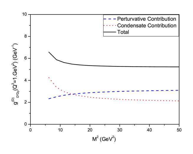
Figure 3: $g^{(D)}_{D^{*}D\rho}(Q^{2}=1.0\,GeV^{2})$ as a function of the Borel mass $M^{2}$.

Using $\Delta_{s}=0.5$ GeV and $\Delta_{u}=0.70\nobreak\,\mbox{GeV}$ for the continuum thresholds and fixing $Q^{2}=1\nobreak\,\mbox{GeV}^{2}$, we found a sum rule for $g_{D^{*}D\rho}^{(D)}$ as a function of $M^{2}$ which is very stable with respect to $M^{2}$ in the interval $20<M^{2}<50\nobreak\,\mbox{GeV}^{2}$. This can be seen in Fig. 3. In what follows we choose the value $M^{2}=30$ GeV² as a reference. In Fig. 4 we show the $M^{2}$ dependence of the form factor $g_{D^{*}D\rho}^{(\rho)}$. Here the threshold parameters were taken to be $\Delta_{s}=\Delta_{u}=0.5$ GeV. Also in this case we find a good stability for a wide range of $M^{2}$ values. We have chosen the Borel mass to be $M^{2}=3$ GeV².

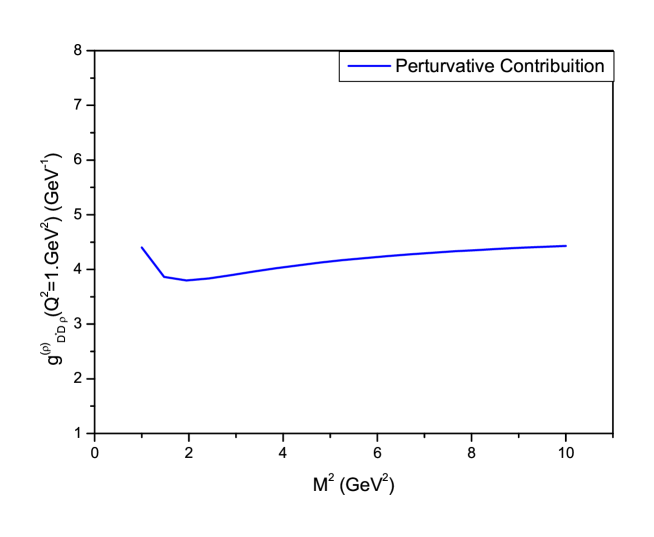
Figure 4: $g^{(\rho)}(Q^{2}=1\nobreak\,\mbox{GeV}^{2})$ as a function of the Borel mass.

Having determined $M^{2}$, we calculated the $Q^{2}$ dependence of the form factors. We present the results in Fig. 5, where the squares correspond to the $g_{D^{*}D\rho}^{(D)}(Q^{2})$ form factor in the interval where the sum rule is valid. The triangles are the result of the sum rule for the $g_{D^{*}D\rho}^{(\rho)}(Q^{2})$ form factor.

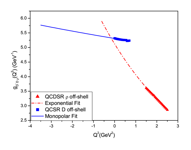
Figure 5: $g^{(D)}_{D^{*}D\rho}$ (squares) and $g^{(\rho)}_{D^{*}D\rho}$ (triangles) QCDSR form factors as a function of $Q^{2}$. The dot-dashed and solid lines correspond to the exponential and monopole parametrizations respectively.

In the case of an off-shell $D$ meson, our numerical results can be fitted by the following monopolar parametrization (shown by the solid line in Fig. 5):

$$g_{D^{*}D\rho}^{(D)}(Q^{2})=\frac{234.38}{Q^{2}+44.14}\;.$$ (20)

where the function $g_{D^{*}D\rho}^{(D)}(Q^{2})$ has the units of GeV^-1, as we could anticipate from (3). Following our previous works bclnn01 ; mnns02 ; mnns05 ; cdnn05 ; bcnn05 , we define the coupling constant as the value of the form factor at $Q^{2}=-m^{2}_{M}$, where $m_{M}$ is the mass of the off-shell meson. Therefore, using $Q^{2}=-m_{D}^{2}$ in Eq (20), the resulting coupling constant is $g^{(D)}_{D^{*}D\rho}=5.76\,\nobreak\,\mbox{GeV}^{-1}$.

For an off-shell $\rho$ meson our sum rule results can be fitted by an exponential parametrization, which is represented by the dot dashed line in Fig. 5:

$$g_{D^{*}D\rho}^{(\rho)}(Q^{2})=5.12e^{-Q^{2}/4.33}\;.$$ (21)

Using $Q^{2}=-m^{2}_{\rho}$ in Eq (21) we get $g^{(\rho)}_{D^{*}D\rho}=5.89\,\nobreak\,\mbox{GeV}^{-1}$.

Looking at Fig. 5 we can observe that the $D$ off-shell form fator is much harder than the $\rho$ off-shell one. This agrees with the conclusions found in most of our previous works: the heavier is the off-shell meson, the harder is its form factor. Every extrapolation introduces some ambiguity in the final results, since we have the freedom to fit a set of points with different parametrizations. In our case this freedom is strongly reduced because we require that both parametrizations lead to the same coupling constant. In Fig. 5 this requirement forces the two endpoints of (20) and (21), which are taken at the squared masses of the corresponding particles, to coincide, i.e., to have the same height in the figure.

In order to study the dependence of our results with the continuum threshold, we vary $\Delta_{s,u}$ between $0.4\nobreak\,\mbox{GeV}\leq\Delta_{s,u}\leq 0.6\nobreak\,\mbox{GeV}$ in the sum rule (18) and $0.4\nobreak\,\mbox{GeV}\leq\Delta_{s}\leq 0.6\nobreak\,\mbox{GeV}$ and $0.65\nobreak\,\mbox{GeV}\leq\Delta_{u}\leq 0.75\nobreak\,\mbox{GeV}$ in the sum rule (19). This variation produces new sets of curves which are shown in Fig. 6 and gives us an uncertainty range in the resultig coupling constants. They are $g_{D^{*}D\rho}^{(D)}=5.70\pm 0.06\,\nobreak\,\mbox{GeV}^{-1}$ and $g_{D^{*}D\rho}^{(\rho)}=5.90\pm 0.08\,\nobreak\,\mbox{GeV}^{-1}$.

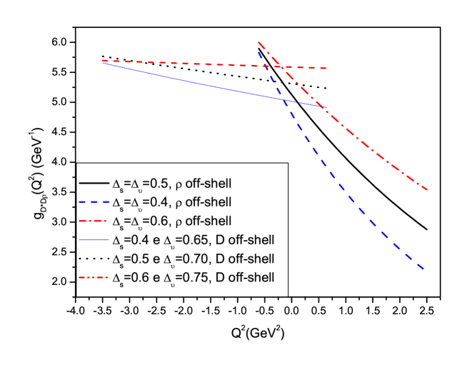
Figure 6: Dependence of the form factor on the continuum thresholds. The solid curve corresponds to $\Delta_{s,u}=0.5\nobreak\,\mbox{GeV}$, the dashed one to $\Delta_{s,u}=0.6\nobreak\,\mbox{GeV}$ and the dotted curve to $\Delta_{s,u}=0.4\nobreak\,\mbox{GeV}$.

We can see that the two cases considered here, off-shell $D$ or $\rho$, give compatible results for the coupling constant. Considering the uncertainties in the continuum thresholds and taking the average between the obtained values we have:

$$g_{D^{*}D\rho}=\Big{(}5.81\pm 0.17\Big{)}\,\nobreak\,\mbox{GeV}^{-1}$$ (22)

Our results were obtained for a concrete choice of currents, Eqs. (10), (11) and (12), which represent charged states. Consequently the obtained couplings are for charged states and from them we can get the generic coupling appearing in the Lagrangian (3) through the relation:

$$g_{D^{*}D\rho}=\frac{g_{\rho^{+}D^{0}D^{*+}}}{\sqrt{2}}=\frac{g_{\rho^{-}D^{0}D^{*+}}}{\sqrt{2}}$$ (23)

Therefore the value of the coupling constant is:

$$g_{D^{*}D\rho}=\Big{(}5.81\pm 0.17\Big{)}/\sqrt{2}=\Big{(}4.13\,\pm 0.08\Big{)}\,\nobreak\,\mbox{GeV}^{-1}$$

In Table II we compare this value with others obtained in previous works. For us the comparison between our results and those found in Ref. wang and Ref. dai02 is especially meaningful, since both approaches use QCD sum rules, although in a different implementation. As it can be seen in Table II, these two works arrive at somewhat different values of the coupling constant, which are, within the errors, compatible with each other. We use the standard SVZ sum rules and the authors of wang ; dai02 work with QCD Light Cone Sum Rules (LCSR). We use the three-point function, whereas they use the two-point function with the $\rho$ as an external field. The advantage of using the three-point function is that it allows us to treat the $\rho$ meson as an off-shell particle and compute not only the coupling constant but also the form factor. Our results have non-perturbative corrections coming from condensates whereas in wang ; dai02 the authors perform a twist expansion. In view of these differences it is reassuring to see that we obtain values of $g_{D^{*}D\rho}$ which are compatible with each other.

This work	LCSR dai02	LCSR wang	VDM su	$SU(4)$ bcnn08
$4.11\pm 0.08$	$4.17\pm 1.04$	$3.56\pm 0.6$	$2.82\pm 0.1$	$3.28\pm 0.1$

Table 2: $g_{D^{*}D\rho}$ in GeV^-1 obtained in previous works.

In Ref. su the authors made an estimate of the ${D^{*}D\rho}$ coupling constant applying the Vector Dominance Model (VDM) to the radiative decay $D^{*}\rightarrow D\gamma$ and using experimental information. The obtained value is somewhat smaller than the others. We should take this estimate with caution, since it has been known since long ago huf that the application of VDM to the charm sector is not always reliable.

Another way to estimate unknown charm coupling constants is to connect them with known couplings through $SU(4)$ relations. In the present case, we could use the relation:

$$g_{D^{*}D\rho}=\frac{g_{D^{*}D^{*}\rho}}{m_{D^{*}}}=\frac{6.6\pm 0.3}{2.01}=\Big{(}3.28\pm 0.15\Big{)}\,\nobreak\,\mbox{GeV}^{-1}$$ (24)

This number is smaller the QCDSR results. In our previous works mnns02 ; bcnn05 we found that, in QCDSR, the $SU(4)$ relation $g_{J/\psi D^{*}D^{*}}=g_{J/\psi DD}$ is satisfied. However, from bclnn01 and bcnn08 we observe that other $SU(4)$ relations, such as $g_{\rho D^{*}D^{*}}=g_{\rho DD}$ and $g_{\rho D^{*}D^{*}}=\frac{\sqrt{6}}{4}g_{J/\psi D^{*}D^{*}}$ are violated at the level of 50 %. This is not surprising since the mass difference starts to play an important role when we go from the heavier vector mesons to $\rho$.

In conclusion, we have calculated the form factors of the $D^{*}D\rho$ vertex and also the coupling constant. We have used QCD sum rules to explore the properties of the three-point Green function of this vertex. The form factors $g_{D^{*}D\rho}^{(D)}(Q^{2})$ (20) and $g_{D^{*}D\rho}^{(\rho)}(Q^{2})$ (21) were obtained for the first time and, as mentioned in the introduction, they can be used in several phenomenological applications. The coupling constant extracted from the form factors is $g_{D^{*}D\rho}=4.1\pm 0.1$ GeV^-1 and it is in agreement with other QCDSR estimates.

- (1) X. Liu, B. Zhang and S. L. Zhu, Phys. Lett. B 645, 185 (2007).
- (2) M.A. Shifman, A.I. and Vainshtein and V.I. Zakharov, Nucl. Phys. B 147, 385 (1979); L.J. Reinders, H. Rubinstein and S. Yazaki, Phys. Rept. 127, 1 (1985); S. Narison, QCD spectral sum rules , World Sci. Lect. Notes Phys. 26, 1 (1989).
- (3) F.S. Navarra, M. Nielsen, M.E. Bracco, M. Chiapparini and C.L. Schat, Phys. Lett. B489, 319 (2000).
- (4) F. S. Navarra, M. Nielsen, M. E. Bracco, Phys. Rev. D65, 037502 (2002).
- (5) M. E. Bracco, M. Chiapparini, A. Lozea, F. S. Navarra and M. Nielsen, Phys. Lett. B521, 1 (2001).
- (6) R.D. Matheus, F.S. Navarra, M. Nielsen and R.R. da Silva, Phys. Lett. B541, 265 (2002).
- (7) R. D. Matheus, F. S. Navarra, M. Nielsen and R. Rodrigues da Silva, Int. J. Mod. Phys. E 14, 555 (2005).
- (8) Z. G. Wang, Nucl. Phys. A 796, 61 (2007); Eur. Phys. J. C 52, 553 (2007); Phys. Rev. D 74, 014017 (2006).
- (9) F. Carvalho, F. O. Durães, F. S. Navarra and M. Nielsen, Phys. Rev. C 72, 024902 (2005).
- (10) M. E. Bracco, M. Chiapparini, F. S. Navarra and M. Nielsen, Phys. Lett. B 605, 326 (2005).
- (11) M. E. Bracco, A. J. Cerqueira, M. Chiapparini, A. Lozea and M. Nielsen, Phys. Lett. B 641, 286 (2006).
- (12) L. B. Holanda, R. S. Marques de Carvalho and A. Mihara, Phys. Lett. B 644, 232 (2007).
- (13) M. E. Bracco, M. Chiapparini, F. S. Navarra and M. Nielsen, Phys. Lett. B 659, 559 (2008).
- (14) Z. Lin and C.M. Ko, Phys. Rev. C62, 034903 (2000); Z. Lin, C.M. Ko and B. Zhang, Phys. Rev. C61, 024904 (2000).
- (15) Y. Oh, T. Song and S.H. Lee, Phys. Rev. C63, 034901 (2001).
- (16) B.L. Ioffe and A.V. Smilga, Nucl. Phys. B216 373 (1983); Phys. Lett. B114, 353 (1982).
- (17) S. Eidelman et al. [Particle Data Group], Phys. Lett. B 592, 1 (2004).
- (18) Z. H. Li, T. Huang, J. Z. Sun and Z. H. Dai, Phys. Rev. D 65, 076005 (2002) [arXiv:hep-ph/0208168].
- (19) J. Hüfner and B. Z. Kopeliovich, Phys. Lett. B 426, 154 (1998).