Shortcut to adiabatic passage in two and three level atoms

Abstract

We propose a method to transfer the population and control the state of two-level and three-level atoms speeding-up Adiabatic Passage techniques while keeping their robustness versus parameter variations. The method is based on supplementing the standard laser beam setup of Adiabatic Passage methods with auxiliary steering laser pulses of orthogonal polarization. This provides a shortcut to adiabaticity driving the system along the adiabatic path defined by the standard setup.

Introduction.—Two major routes for manipulating the state of a quantum system with interacting fields are based on resonant pulses or on adiabatic methods, such as “Rapid” Adiabatic Passage (RAP), Stimulated Raman Adiabatic Passage (STIRAP) and their many variants. In general terms simple fixed-area resonant pulses may be fast if intense enough, but quite unstable with respect to errors or fluctuations of the parameters, whereas adiabatic passage is robust but slow. For many applications, from Nuclear Magnetic Resonance (NMR) to quantum information processing, the ideal method should be fast and robust, combining the best of the two worlds. These two requirements are particularly demanding if quantum computing is to become feasible at all. It is possible to make the pulses more stable by combining them into pulse sequences, but in practice their use is limited by the longer times required with respect to the single pulse, the need to control phase angles and pulse durations accurately, or off-resonant excitations due to sharp pulse edges NMR . Moreover the error compensating properties of square-pulse sequences are not preserved when substituting them with smooth pulses so that the design of good sequences requires “a good portion of experience and magic” Molmer . In NMR, composite pulses are increasingly superseded by adiabatic passage methods NMR , which have also been very successful in chemical reaction dynamics Kral , laser cooling lc , atom optics RM , metrology Salomon , interferometry Chu , or cavity quantum electrodynamics Lambro ; Bergmann . When robustness is the primary concern, they are quite sufficient, and have as well become basic operations for quantum information processing, either to design robust gates JJ ; gates or in quantum adiabatic computing AC1 ; AC2 , which relies on an adiabatic evolution of the ground state from an initial to a final Hamiltonian. If speed is also important, however, the limitations may be severe AC2 . Given the stated difficulties of composite pulses, it is then quite natural to look for robustness and high operation velocities taking the adiabatic methods as the starting point and shortening their duration somehow. Our objective here is to propose a shortcut to adiabatic passage (abbreviated as “SHAPE” hereafter) using a recent formulation by Berry Berry09 of “transitionless quantum driving”, related to work by Kato Kato on the adiabatic theorem. The specific applications we shall discuss are speeded-up versions of (2-level) RAP and (3-level) STIRAP schemes, as canonical examples of other adiabatic methods. Variants such as fractional RAP or STIRAP, and multilevel schemes may be treated along similar lines.

The philosophy of the transitionless quantum driving algorithm Berry09 is to supplement the Hamiltonian $H_{0}(t)$ of a reference system with an auxiliary term $H_{1}(t)$ to steer the dynamics exactly along the instantaneous eigenstates $|\lambda_{n}(t)\rangle$ of $H_{0}(t)$ without transitions among them, formally in an arbitrarily short time,

$$H_{1}(t)=i\hbar\sum_{n}(|\partial_{t}\lambda_{n}\rangle\langle\lambda_{n}|-\langle\lambda_{n}|\partial_{t}\lambda_{n}\rangle|\lambda_{n}\rangle\langle\lambda_{n}|).$$ (1)

At variance with Lyapunov-control methods Wang , the extra term is independent of the time-dependent state so it leads to simpler, linear dynamics, and moreover it provides systematically exact solutions for adiabatic following without the need for a trial and error approach to find a good control field Wang . Regarding its physical realizability, in general there is no guarantee that $H_{1}$ may be easy to implement and each case needs a separate study. For example, for an $H_{0}$ describing a particle in a time-dependent harmonic potential, $H_{1}$ turns out to be a non-local interaction, and its realizability in a useful parameter domain for cold atoms remains an open question JPB2 . (Transitionless dynamics for the harmonic oscillator may be achieved with a local interaction by inverse engineering the frequency dependence with the aid of Ermakov-Riesenfeld invariants Xi , or with state acceleration techniques Nakamura .) For a particle with spin in a time dependent magnetic field, $H_{1}$ becomes a complementary, time-dependent magnetic field Berry09 . For the atomic two- and three-level systems studied here, $H_{1}$ will involve laser interactions added to the original laser setup implied by $H_{0}$ as discussed below.

Rapid Adiabatic Passage.—Let us consider first the speeding-up of a standard Rapid Adiabatic Passage that inverts the population of two-levels of an atom, $|0\rangle$ and $|1\rangle$, by sweeping the radiation through resonance. This broadspread technique originated in Nuclear Magnetic Resonance Bloch but is used in virtually all fields where 2-level systems may be controlled by external interactions, such as laser-chemistry, modern quantum optics or quantum information processing. When the frequency sweep is much shorter than the life-time for spontaneous emission and other relaxation times, it is termed rapid adiabatic passage (RAP).

Using the rotating wave approximation, the Hamiltonian ${H}_{0}(t)$ in a laser-adapted interaction picture can be written as

$${H}_{0}(t)=\frac{\hbar}{2}\left(\begin{array}[]{cc}\Delta(t)&\Omega_{R}(t)\\ \Omega_{R}(t)&-\Delta(t)\end{array}\right),$$ (4)

where $\Omega_{R}(t)$ is the Rabi frequency, which we take to be real, and $\Delta(t)=\omega_{0}-\omega_{L}$ the detuning, assumed to change slowly on the scale of the optical period. It is the difference between the Bohr transition frequency and the laser carrier frequency $\omega_{L}$, due to a change in the carrier frequency or a controlled alteration of the Bohr frequency by Zeeman or Stark shifts. The instantaneous eigenvectors are

$$|\lambda_{+}(t)\rangle = \cos[\theta(t)/2]|1\rangle-\sin[\theta(t)/2]|0\rangle,$$ (5)

$$|\lambda_{-}(t)\rangle = \sin[\theta(t)/2]|1\rangle+\cos[\theta(t)/2]|0\rangle,$$ (6)

with the mixing angle $\theta(t)\equiv\arccos[-\Delta(t)/\Omega(t)]$ and eigenvalues $E_{\pm}(t)=\pm\hbar\Omega/2$, where $\Omega=\sqrt{\Delta^{2}(t)+\Omega^{2}_{R}(t)}$. If the adiabaticity condition

$$\frac{1}{2}|\Omega_{a}|\ll|\Omega(t)|,$$ (7)

where $\Omega_{a}\equiv[\Omega_{R}(t)\dot{\Delta}(t)-\dot{\Omega}_{R}(t)\Delta(t)]/\Omega^{2}$, is satisfied, the state evolving from $|\psi(t=0)\rangle=|\lambda_{\pm}(0)\rangle$ follows the adiabatic approximation

$$|\psi_{\pm}(t)\rangle=\exp{\left\{-\frac{i}{\hbar}\int^{t}_{0}dt^{\prime}E_{\pm}(t^{\prime})\right\}}|\lambda_{\pm}(t)\rangle,$$ (8)

whereas transitions will occur otherwise. Different adiabatic passage schemes correspond to different specifications of $\Omega_{R}$ and $\Delta$ for which $\psi_{\pm}$ passes from one bare state to the other. The simplest one is the Landau-Zener scheme with constant $\Omega_{R}$ and linear-in-time $\Delta$. For the examples below we shall use the more adiabatic (and thus potentially faster) Allen-Eberly scheme AE ; VG : $\Omega_{R}=\Omega_{0}\operatorname{sech}(\pi t/2t_{0})$, $\Delta=(2\beta^{2}t_{0}/\pi)\tanh(\pi t/2t_{0})$. Regardless of the scheme chosen ${H}_{1}(t)$ takes the form

$${H}_{1}(t)=\frac{\hbar}{2}\left(\begin{array}[]{cc}0&-i\Omega_{a}\\ i\Omega_{a}&0\end{array}\right),$$ (11)

where (up to a phase factor) $\Omega_{a}$ plays the role of the Rabi frequency of the auxiliary field. In principle $H=H_{0}+H_{1}$ drives the dynamics along the $H_{0}$-adiabatic path in arbitrarily short times, but there are practical limitations such as the laser power available. Moreover, a comparison with $H_{0}$-dynamics is only fair if $|\Omega_{a}|$ is smaller or approximately equal to the peak Rabi frequency with the original laser setup. Independently of the scheme chosen and in a range of interaction times that break down the adiabaticity condition, it is remarkable that the dynamics can be driven along the $H_{0}$-adiabatic path while fulfilling the inequalities $|\Omega_{a}|\leq|\Omega|\leq|\Omega_{0}|$.

The physical meaning and realizability of the auxiliary term are determined by going back to the Schrödinger picture: it represents a laser with the same time dependent frequency of the original one, but a differently shaped time-dependent intensity, and perpendicular polarization.

For the Allen-Eberly scheme the population of the excited state $P_{1}$ starting from the ground state depends on the dimensionless parameters $\tau=t_{0}\beta$ and $\omega=\Omega_{0}/\beta$ VG : $P_{1}=1-\operatorname{sech}^{2}(2\tau^{2}/\pi)\cos^{2}[\tau(\omega^{2}-4\tau^{2}/\pi^{2})^{1/2}]$. A population transfer near to one ($P_{1}>0.999$) and stable versus parameter variations is achieved for $\omega\geq 3$ and $\tau\geq 3$. We may calculate $\Omega_{a}$ and the minimal time for which the maximum of $\Omega_{a}$ with respect to $t$ is $\leq\Omega_{0}$. In the stated range this is accurately given by $\tau_{m}=\pi/(4\omega)$, or $t_{0,m}=\pi/(4\Omega_{0})$. The reduction factor with respect to the adiabatic time $\tau_{a}\approx 3$ may be very significant, $t_{0,m}/t_{a}\approx{\pi}/{(12\omega)}$, this is $0.09$ for $\omega=3$, or $0.01$ for $\omega=20$. Of course the SHAPE Hamiltonian $H$ may also drive the system along the adiabatic path outside the $w,\tau>3$ domain as illustrated in Fig. 1.

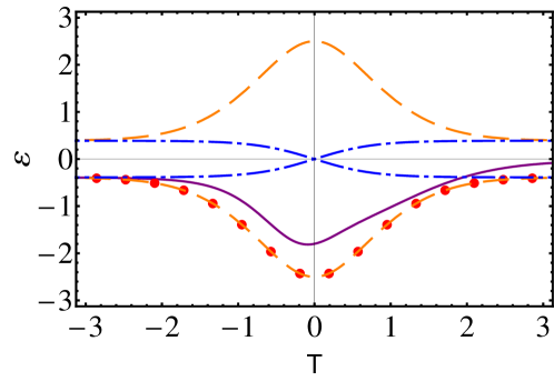
Figure 1: (color online). (Dimensionless) energies $\varepsilon=E/(\beta\hbar)$ versus (dimensionless) time $T=t\beta$ for the AE scheme: Diabatic energies, dot-dashed (blue) lines; adiabatic energies, dashed (orange) lines; average energy evolving with $H_{0}$, solid (purple) line; average energy evolving with $H=H_{0}+H_{1}$, dotted (red) line, indistinguishable from the lower adiabatic energy. $\omega=5$, $\tau=1.22$.

For comparison, the population of the excited state due to a square $\pi$ pulse with on-resonance Rabi frequency $\Omega_{0}$ is

$$P_{1}=\frac{\Omega_{0}}{\Omega}\left|\sin\left(\frac{\Omega t}{2}\right)\right|^{2}.$$ (12)

Complete population transfer requires $\Delta=0$, and a pulse time $t_{R}=\frac{\pi}{\Omega_{0}}$. For the same $\Omega_{0}$ and limiting the auxiliary laser by $|\Omega_{a}|\leq\Omega_{0}$, the minimal characteristic time $t_{0,m}$ of the SHAPE method is of the order of $t_{R}$, $t_{0,m}=t_{R}/4$. In fact the actual interaction time to implement a successful population inversion with the AE scheme (SHAPE corrected or not) should be a few times $t_{0}$; this may be estimated from the dependence of the excited population of the adiabatic state with time, which is $>.999$ for $t\geq 8t_{0}$.

Figures 2 and 3 show examples of the fidelity ($P_{1}$) with respect to variations in the Rabi frequency and detuning with SHAPE (AE scheme for $H_{0}$), the evolution with $H_{0}$ (AE scheme), a Rabi $\pi$-pulse, and a composite $\frac{\pi}{2}(x)\pi(y)\frac{\pi}{2}(x)$ pulse, a fault-tolerant combination where $x,y$ refer to the laser polarization (and Pauli matrix) involved. Clearly SHAPE provides a fast, robust and efficient population inversion compared to all other methods. All cases are for the same $\Omega_{0}$, and in SHAPE $|\Omega_{a}|\leq\Omega_{0}$.

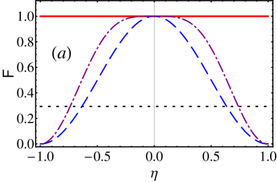
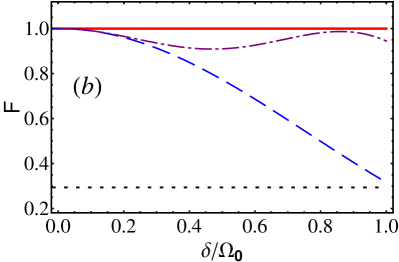
Figure 2: (color online). Dependence of the fidelity ($P_{1}$) on the changes of (a) the Rabi frequency from $\Omega_{0}$ to $\Omega_{0}(1+\eta)$ (b): the detuning by $\delta$. SHAPE, AE scheme (solid, red line) with $\Omega_{a}\leq\Omega_{0}$; ordinary Adiabatic Passage (dotted, black line); Rabi pulse (dashed, blue line); Composite pulse $\frac{\pi}{2}(x)\pi(y)\frac{\pi}{2}(x)$ (dot-dashed, purple line). $\Omega_{0}=2\pi\times 5$ MHz; $t_{0}=25$ ns; $\beta=2\pi$ MHz.

Stimulated Raman Adiabatic Passage.—Similar ideas can be applied to three-level STIRAP. The Hamiltonian ${H}_{0}(t)$ for the two-photons resonance case within the rotating wave approximation (RWA) and in a laser adapted interaction picture reads Bergmann

$${H}_{0}(t)=\frac{\hbar}{2}\left(\begin{array}[]{ccc}0&\Omega_{p}(t)&0\\ \Omega_{p}(t)&2\Delta&\Omega_{s}(t)\\ 0&\Omega_{s}(t)&0\end{array}\right),$$ (16)

in terms of the Rabi frequencies for the Stokes, $\Omega_{s}(t)$, and pumping lasers, $\Omega_{p}(t)$, and the laser detuning $\hbar\Delta=(E_{2}-E_{1})-\hbar\omega_{p}=(E_{2}-E_{3})-\hbar\omega_{s}$. The instantaneous eigenstates $|\lambda_{n}\rangle$ are

$$|\lambda_{+}(t)\rangle = \sin\theta\sin\phi|1\rangle+\cos\phi|2\rangle+\cos\theta\sin\phi|3\rangle,$$

$$|\lambda_{-}(t)\rangle = \sin\theta\cos\phi|1\rangle-\sin\phi|2\rangle+\cos\theta\cos\phi|3\rangle,$$

$$|\lambda_{0}(t)\rangle = \cos\theta|1\rangle-\sin\theta|3\rangle,$$ (17)

with eigenvalues given by $E_{+}(t)=\hbar\Omega\cot(\phi/2)$, $E_{0}=0$, and $E_{-}(t)=-\hbar\Omega\tan(\phi/2)$. The time-dependent mixing angles $\theta$ and $\phi$ are respectively defined by $\tan\theta=\Omega_{p}(t)/\Omega_{s}(t)$ and $\tan(2\phi)=\Omega/\Delta(t)$, whereas $\Omega=\sqrt{\Omega^{2}_{p}(t)+\Omega^{2}_{s}(t)}$. The population transfer $1\rightarrow 3$ is realized by the “dark state” $|\lambda_{0}\rangle$.

The Hamiltonian ${H}_{1}(t)$, takes now the form

$${H}_{1}(t)=i\hbar\left(\begin{array}[]{ccc}0&\dot{\phi}\sin\theta&\dot{\theta}\\ -\dot{\phi}\sin\theta&0&-\dot{\phi}\cos\theta\\ -\dot{\theta}&\dot{\phi}\cos\theta&0\end{array}\right),$$ (21)

with $\dot{\theta}=[{\dot{\Omega}_{p}(t)\Omega_{s}(t)-\dot{\Omega}_{s}(t)\Omega_{p}(t)}]/{\Omega^{2}},$ and $\dot{\phi}=[{(\dot{\Omega}_{p}(t)\Omega_{p}(t)+\dot{\Omega}_{s}(t)\Omega_{s}(t))\Delta(t)}]/[{2\Omega(\Delta^{2}+\Omega^{2})}].$ We would need in principle three new lasers to implement this Hamiltonian. The ones connecting levels $1$-$2$ and $2$-$3$ should have the same frequency as the original ones but orthogonal polarization, and the field connecting levels $1$-$3$ should be on resonance with this transition to get an interaction picture Hamiltonian like (21) (The RWA approximation is assumed in all cases.) If $1$-$3$ is electric-dipole-forbidden, a magnetic dipole transition may be used instead. If we are only interested in performing a full passage from 1 to 3 and do not want to reproduce all the effects of the full Hamiltonian $H_{0}+H_{1}$, $H_{1}$ may be simplified by retaining just the $1$-$3$ interaction,

$${H}^{\prime}_{1}(t)=\frac{\hbar}{2}\left(\begin{array}[]{ccc}0&0&i\Omega^{\prime}_{a}\\ 0&0&0\\ -i\Omega^{\prime}_{a}&0&0\end{array}\right),$$ (22)

where $\Omega^{\prime}_{a}=2\dot{\theta}$. That this is so may be seen by working out the Schrödinger equation in the adiabatic basis: $d\langle\lambda_{0}(t)|\psi(t)\rangle/dt$ does not depend on $\dot{\phi}$ so that the $1$-$3$ and $2$-$3$ auxiliary lasers can be left out without affecting $\langle\lambda_{0}(t)|\psi(t)\rangle$. In the examples below we have chosen the pulse shapes Fewell

$$\Omega_{p}(t) = \Omega_{0}(t)f(t-\tau);~{}~{}\Omega_{s}(t)=\Omega_{0}(t)f(t),$$

$$f(t) = \left\{\begin{array}[]{ll}\sin^{4}(\pi t/{\sf{T}}){}{}&(0<t<{\sf T}),\\ 0{}{}{}{}{}&(\mbox{otherwise).}\end{array}\right.$$ (25)

Fig. 3 shows a STIRAP Stokes-Pump pulse sequence where ${\sf T}$ is too short for complete population transfer because adiabaticity breaks down, see Fig. 4a. We can remedy that with the auxiliary interaction in (22), see Figs. 3 and 4b. Keeping $|\Omega_{a}^{\prime}|\leq\Omega_{0}$ the process duration is reduced approximately ten times with respect to the ordinary STIRAP scheme.

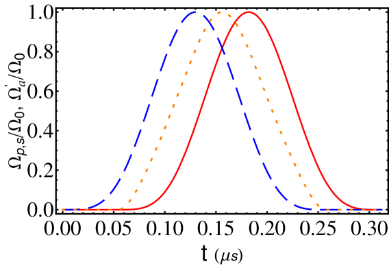
Figure 3: (color online). Time evolution of Rabi frequencies in a STIRAP sequence of laser pulses defined by Eq. (25) with $\Omega_{0}=2\pi\times 5$ MHz, $\Delta=2\pi\times 0.5$ MHz, and ${\sf T}=0.26$ $\mu$s. Dashed blue line: $\Omega_{s}/\Omega_{0}$; Solid red line: $\Omega_{p}/\Omega_{0}$; The dotted orange curve represents $\Omega^{\prime}_{a}/\Omega_{0}$.

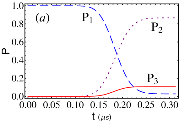
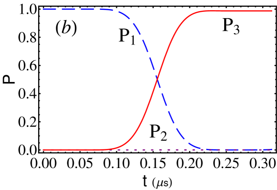
Figure 4: (color online). Time evolution of the populations of levels 1, 2 and 3 for STIRAP: (a) Hamiltonian ${H}_{0}(t)$; (b) Hamiltonian ${H}(t)$ with additional ${H}_{1}(t)$. Same parameters as in Fig. 3.

Discussion and conclusions.—A method to achieve fast and robust population transfer in two-level and three-level atomic systems has been presented, based on supplementing the laser setup of standard adiabatic passage methods (RAP or STIRAP) by additional, properly time-shaped pulses with orthogonal polarization. The Hamiltonian $H_{1}(t)$ that describes the additional steering pulses providing a shortcut to adiabaticity is given by a general algorithm to drive quantum systems without transitions Berry09 . Other states (such as superpositions of two-levels) may be prepared by speeded-up (SHAPE) versions of fractional RAP or STIRAP, and, if necessary, the phases may be controlled thanks to the freedom to choose the reference Hamiltonian $H_{0}(t)$ or phase gates. As an outlook, similar techniques may provide a way to carry out adiabatic computation in a finite time Aha ; bra , or to speed up logic gates based on adiabatic processes CBZ ; Ion , interferometric techniques in superconducting qubits Shevchenko or quantum dots Jong , and the creation of entangled pairs of two-state systems Unanyan . The SHAPE method is compatible with approaches that optimize $H_{0}$ such as the quantum brachistochrone approach Zan , since, after optimizing the adiabatic process, it leads to the design of even faster process. Other adiabatic techniques SCRAP may also benefit from these ideas speeding up the avoided level crossings and keeping their stability versus parameter variations.

We thank M. V. Berry and J. H. Eberly for discussions, and acknowledge funding by Projects No. GIU07/40, No. FIS2009-12773-C02-01, No. NSFC 60806041, No. 08QA14030, No. 2007CG52, No. S30105, No. ANR-09-BLAN-0134-01, and Juan de la Cierva Program.

References

- (1) T. D. W. Claridge, High-resolution NMR techniques in organic chemistry, 2nd edition, Elsevier 2009, Amsterdam.
- (2) I. Roos and K. Molmer, Phys. Rev. A 69, 022321 (2004).
- (3) P. Král, I. Thanopulos, and M. Shapiro, Rev. Mod. Phys. 79, 53 (2007).
- (4) H. J. Metcalf and P. van der Straten, Laser Cooling and Trapping, Springer 1999, New York.
- (5) A. Ruschhaupt and J. G. Muga, Phys. Rev. A 73, 013608 (2006).
- (6) F. Pereira Dos Santos et al., Phys. Rev. Lett. 89, 233004 (2002).
- (7) M. Weitz, B. C. Young, and S. Chu, Phys. Rev. Lett. 73, 2563 (1994).
- (8) P. Lambropoulos and D. Petrosyan, Fundamentals of Quantum Optics and Quantum Information, Springer 2007, Berlin.
- (9) K. Bergmann, H. Theuer, and B. W. Shore, Rev. Mod. Phys. 70, 1003 (1997).
- (10) J. García-Ripoll and I. Cirac, Phys. Rev. Lett. 90, 12902 (2003).
- (11) X. Lacour et al., J. Phys. IV France 135, 209 (2006).
- (12) E. Farhi et al., Science 292, 472 (2001).
- (13) D. Aharonov et al., Proc. 45th FOCS, 42 (2004).
- (14) M. V. Berry, J. Phys. A: Math. Theor. 42, 365303 (2009).
- (15) T. Kato, J. Phys. Soc. Japan, 5, 435 (1950).
- (16) W. Wang, S. C. Hou, and X. X. Yi, arXiv:0910.5859v1.
- (17) J. G. Muga et al., J. Phys. B: At. Mol. Opt. Sci, accepted.
- (18) X. Chen et al., Phys. Rev. Lett. 104, 063002 (2010).
- (19) S. Masuda and K. Nakamura, Proc. R. Soc. A 466, 1135 (2010).
- (20) F. Bloch, Phys. Rev. 70, 460 (1946).
- (21) L. Allen and J. H. Eberly, Optical resonance and two-level atoms, Dover Publications, INC., New York, 1987.
- (22) N. V. Vitanov and B. M. Garraway, Phys. Rev. A 53, 4288 (1996).
- (23) M. P. Fewell, B. W. Shore, and K. Bergmann, Aust. J. Phys. 50, 281 (1997).
- (24) D. Aharonov, SIAM J. Comput. 37, 166 (2007).
- (25) A. T. Rezakhani et al., Phys. Rev. Lett. 103, 080502 (2009).
- (26) J. I. Cirac, R. Blatt, and P. Zoller, Phys. Rev. A 49, R3174 (1994).
- (27) I. Lizuain, J. G. Muga, Phys. Rev. A 75, 033613 (2007).
- (28) S. N. Shevchenko, S. Ashhab, and F. Nori, arXiv:0911.1917v1.
- (29) L. M. Jong and A. D. Greentree, Phys. Rev. B 81, 035311 (2010).
- (30) R. G. Unanyan, N. V. Vitanov, and K. Bergmann, Phys. Rev. Lett. 87, 137902 (2001).
- (31) A. T. Rezakhani et al., Phys. Rev. Lett. 103, 080502 (2009).
- (32) L. P. Yatsenko et al., Phys. Rev. A 60, R4237, (1999).