1 Introduction

The last few years have witnessed a remarkable progress in our understanding of the non-Abelian vortices and their relation to monopoles, both of which are thirty-year old problems in theoretical physics, and which can bear important implications to some deep issues such as quark confinement. The plan of this talk is: (i) a very brief review of non-Abelian monopoles; (ii) a brief review of ’03-’07 results on non-Abelian vortices; (iii) a new result on non-Abelian vortices based on general gauge groups; (iv) the fractional vortices; and (v) a brief discussion on the monopole-vortex complex and non-Abelian duality.

It has become customary to think of quark confinement as a dual superconductor, in which (chromo-) electric charges are confined in a medium in which a magnetic charge is condensed. The original suggestion by ’t Hooft and Mandelstam is essentially Abelian: the effective low-energy degrees of freedom are magnetic monopoles arising from the Yang-Mills gauge fields. It is however possible that the dual superconductor relevant to quark confinement is of a non-Abelian kind, in which case we must better understand the quantum mechanical properties of these degrees of freedom. We would like to understand how the ’t Hooft-Polyakov monopoles [1] (arising from a gauge symmetry breaking, $G\to H$) and Abrikosov-Nielsen-Olesen vortices [2] (of a broken gauge theory $H\to\mathbbm{1}$) are generalized in situations where the relevant gauge group $H$ is non-Abelian.

The key developments which allowed us a qualitatively better understanding of these solitons are the following. First, the Seiberg-Witten solutions of ${\cal N}=2$ supersymmetric gauge theories [3, 4] revealed the quantum-mechanical behavior of the magnetic monopoles in an unprecedented fashion. In the presence of matter fields (quarks and squarks) these theories have, typically, vacua with non-Abelian dual gauge symmetry in the infrared [5, 6]. Thus in these systems non-Abelian monopoles do exist and play a central role in confinement and dynamical symmetry breaking. Second, the discovery of non-Abelian vortex solutions [7, 8], i.e., soliton vortices with continuous, non-Abelian moduli, has triggered an intense research activity on the classical and quantum properties of these solitons, leading to a rich variety of new interesting results [9, 10, 11].

2 Monopoles

When the gauge symmetry is spontaneously broken

$$G\,\,\,{\stackrel{{\scriptstyle\langle\phi_{1}\rangle\neq 0}}{{\longrightarrow}}}\,\,\,H$$ (1)

where $H$ is some non-Abelian subgroup of $G$, the system possesses a set of regular magnetic monopole solutions in the semi-classical approximation. They are natural generalizations of the Abelian ’t Hooft-Polyakov monopoles [1], found originally in the $G=SO(3)$ theory broken to $H=U(1)$ by a Higgs mechanism. The gauge field looks asymptotically as

$$F_{ij}=\epsilon_{ijk}B_{k}=\epsilon_{ijk}\frac{r_{k}}{r^{3}}({\beta}\cdot{\bf H}),$$ (2)

in an appropriate gauge, where ${\bf H}$ are the diagonal generators of $H$ in the Cartan subalgebra. A straightforward generalization of the Dirac’s quantization condition leads to [12]

$$2\,{\beta\cdot\alpha}\in{\bf Z}$$ (3)

where $\alpha$ are the root vectors of $H$. In the simplest such case, $G=SU(3)$, $H=SU(2)\times U(1)/{\mathbbm{Z}}_{2}\sim U(2)$, a straightforward idea that the degenerate monopole solutions to be a doublet of the unbroken $SU(2)$ leads however to the well-known difficulties [14, 15].

On the other hand, the quantization condition Eq. (3) implies that the monopoles should transform, if any, under the dual of $U(2)$: the individual solutions are labelled by $\beta$ which live in the weight vector space of ${\tilde{H}}$, generated by the dual roots,

$$\alpha^{*}=\frac{\alpha}{\alpha\cdot\alpha}.$$ (4)

As transformation groups of fields $H$ and $\tilde{H}$ are relatively non-local, the sought-for transformations of monopoles must look as non-local field transformations from the point of view of the original theory [16].

But the most significant fact is that fully quantum mechanical monopoles appears in the low-energy dual description of a wide class of ${\cal N}=2$ supersymmetric QCD [5, 6]. There must be ways to understand the physics of non-Abelian monopoles starting from a more familiar, semiclassical soliton picture.

3 Vortices

Attempts to understand the semi-classical origin of the non-Abelian monopoles appearing in the so-called $r$-vacua of the ${\cal N}=2$ supersymmetric $SU(N)$ gauge theory, has eventually led to the discovery of the non-Abelian vortices [7, 8]. They are natural generalizations of the Abrikosov-Nielsen-Olesen (ANO) vortex. Unlike the ANO vortex, however, the non-Abelian vortices carry continuous zeromodes, i.e., it has a nontrivial moduli.

The simplest model in which these vortices appear is an $SU(N)\times U(1)$ gauge theory with $N_{f}=N$ flavors of squarks in the fundamental representation. The secret of the non-Abelian vortices lies in the so-called color-flavor locked phase, in which the squark fields (written as $N\times N$ color-flavor mixed matrix) takes the VEV of the form,

$$\langle q(x)\rangle=v\,{\mathbbm{1}}_{N\times N}\;.$$ (5)

The $SU(N)$ gauge symmetry is completely broken, but the color-flavor mixed diagonal symmetry remains unbroken.

The vortex configuration in this vacuum involves scalar fields of the form,

$$q(x)=v\,\left(\begin{array}[]{cccc}e^{i\phi}\,f(\rho)&0&0&0\\ 0&g(\rho)&0&0\\ 0&0&\ddots&0\\ 0&0&0&g(\rho)\end{array}\right)$$ (6)

where $\rho,\phi,z$ (the static vortex does not depend on $z$) are the cylindrical coordinates. The gauge fields take appropriate form, in order to ensure that the kinetic term tends to zero asymptotically, ${\cal D}q(x)\to 0$. In Eq. (6) the first flavor of the squark winds, but the full solution $A_{i},q(x)$ can be rotated in the color flavor $SU(N)$ transformations,

$$A_{i},\to U(A_{i}+i\partial_{i})U^{\dagger},\qquad q(x)\to Uq(x)U^{\dagger}\;,$$

leaving the tension invariant.

In other words, individual vortices break the exact $SU(N)_{C+F}$ symmetry of the system, developing therefore non-Abelian orientational zeromodes. Its nature is seen from the fact that the vortex Eq. (6) breaks the global symmetry as

$$SU(N)\to SU(N-1)\times U(1)/{\mathbbm{Z}}_{N-1};$$ (7)

the vortex moduli is given by

$$CP^{N-1}\sim\frac{SU(N)}{SU(N-1)\times U(1)/{\mathbbm{Z}}_{N-1}}\;.$$ (8)

They are Nambu-Goldstone modes, which however can propagate only inside the vortex: far from it they are massive.

The quantum properties of the non-Abelian orientational modes (the effective $CP^{N-1}$ sigma model), the study of non-Abelian vortices of higher winding numbers, the generalization to the cases of larger number of flavors and the study of the resulting, much richer vortex moduli spaces, the question of vortex stability in the presence of small non-BPS corrections, extension to more general class of gauge theories, etc. have been the subjects of an intense research activity recently.

4 Non-Abelian vortices with general gauge groups

One of the new results by us [17] is the construction of non-Abelian vortex solutions based on a general gauge group $G^{\prime}\times U(1)$, where $G^{\prime}=SU(N),$ $SO(N),$ $USp(2N)$, etc. As in models based on $SU(N)$ gauge groups studied extensively in the last few years, we work with simple models which have the structure of the bosonic sector of $N=2$ supersymmetric models. The model contains a FI (Fayet-Iliopoulos)-like term in the $U(1)$ sector, allowing the system to develop stable vortices. A crucial aspect is that we work in a complete Higg vacuum, but with an unbroken color-flavor diagonal symmetry. We take as our model system

$$\cal{L} = \hbox{\rm Tr}_{c}\Big{[}-\frac{1}{2e^{2}}F_{\mu\nu}F^{\mu\nu}-\frac{1}{2g^{2}}\hat{F}_{\mu\nu}\hat{F}^{\mu\nu}+\cal{D}_{\mu}H\left(\cal{D}^{\mu}H\right)^{\dagger}$$

$$-\frac{e^{2}}{4}\left|X^{0}t^{0}-2\xi t^{0}\right|^{2}-\frac{g^{2}}{4}\left|X^{a}t^{a}\right|^{2}\Big{]}\ ,$$

with the field strength, gauge fields and covariant derivative denoted as

$$F_{\mu\nu} = F_{\mu\nu}^{0}t^{0}\,,\quad F_{\mu\nu}^{0}=\partial_{\mu}A_{\nu}^{0}-\partial_{\nu}A_{\mu}^{0}\ ,\quad\hat{F}_{\mu\nu}=\partial_{\mu}A_{\nu}-\partial_{\nu}A_{\mu}+i\left[A_{\mu},A_{\nu}\right],$$

$$A_{\mu} = A_{\mu}^{a}t^{a}\ ,\quad{\cal D}_{\mu}=\partial_{\mu}+iA_{\mu}^{0}t^{0}+iA_{\mu}^{a}t^{a},$$

$A_{\mu}^{0}$ is the gauge field associated with $U(1)$ and $A_{\mu}^{a}$ are the gauge fields of $G^{\prime}$. The matter scalar fields are written as an $N\times N_{\rm F}$ complex color (vertical) – flavor (horizontal) mixed matrix $H$. It can be expanded as $X=HH^{\dagger}=X^{0}t^{0}+X^{a}t^{a}+X^{\alpha}t^{\alpha}\ \,\,$, $X^{0}=2\,\hbox{\rm Tr}_{c}\left(HH^{\dagger}t^{0}\right)$, $X^{a}=2\,\hbox{\rm Tr}_{c}\left(HH^{\dagger}t^{a}\right)$. $t^{0}$ and $t^{a}$ stand for the $U(1)$ and $G^{\prime}$ generators, respectively, and finally, $t^{\alpha}\in\mathfrak{g}^{\prime}_{\perp}$, where $\mathfrak{g}^{\prime}_{\perp}$ is the orthogonal complement of the Lie algebra $\mathfrak{g}^{\prime}$ in $\mathfrak{su}(N)$. The traces with subscript $c$ are over the color indices. $e$ and $g$ are the $U(1)$ and $G^{\prime}$ coupling constants, respectively, while $\xi$ is a real constant.

We choose the maximally “color-flavor-locked” vacuum of the system,

$$\langle H\rangle=\frac{v}{\sqrt{N}}{\bf 1}_{N}\ ,\qquad\xi=\frac{v^{2}}{\sqrt{2N}}\,.$$ (9)

We have taken $N_{\rm F}=N$ which is the minimal number of flavors allowing for such a vacuum. Note that, unlike the $U(N)$ model studied extensively in the last several years, the vacuum is not unique in these cases (i.e., with a general gauge group), even with such a minimum choice of the flavor multiplicity. This difference may be traced to the fact that groups such as $SO(N)\times U(1)$ and $USp(N)\times U(1)$ form strictly smaller subgroups of $U(N)$.

The existence of a continuous vacuum degeneracy implies the emergence of vortices of semi-local type; this aspect will be crucial in the discussion of the fractional vortices in the second part of this talk. However, for now, we stick to the particular vacuum Eq. (9) and consider vortices and their moduli in this theory. The standard Bogomol’nyi completion reads

$$T = \int d^{2}x\,\hbox{\rm Tr}_{c}\Big{[}\frac{1}{e^{2}}\left|F_{12}-\frac{e^{2}}{2}\left(X^{0}t^{0}-2\xi t^{0}\right)\right|^{2}+\frac{1}{g^{2}}\left|\hat{F}_{12}-\frac{g^{2}}{2}\,X^{a}t^{a}\right|^{2}$$ (10)

$$+4\left|\bar{\cal{D}}H\right|^{2}-2\xi F_{12}t^{0}\Big{]}\geq-\xi\int d^{2}x\,F^{0}_{12}\ ,$$

where $\bar{\cal D}\equiv\frac{{\cal D}_{1}+i{\cal D}_{2}}{2}$, $z=x^{1}+ix^{2}$. In the BPS limit one has

$$T=2\sqrt{2N}\pi\xi\nu=2\pi v^{2}\nu\ ,\qquad\nu=-\frac{1}{2\pi\sqrt{2N}}\int d^{2}x\,F_{12}^{0}\ ,$$ (11)

where $\nu$ is the $U(1)$ winding number of the vortex. This leads immediately to the vortex BPS equations

$$\bar{\cal{D}}H = \bar{\partial}H+i\bar{A}H=0\ ,$$ (12)

$$F_{12}^{0} = e^{2}\left[\,\hbox{\rm Tr}_{c}\left(HH^{\dagger}t^{0}\right)-\xi\,\right]\ ,\qquad F_{12}^{a}=g^{2}\,\hbox{\rm Tr}_{c}\left(HH^{\dagger}t^{a}\right)\ .$$ (13)

The matter BPS equation (12) can be solved by the Ansatz

$$H=S^{-1}(z,\bar{z})H_{0}(z)\ ,\qquad\bar{A}=-iS^{-1}(z,\bar{z})\bar{\partial}S(z,\bar{z})\ ,$$ (14)

where $S$ belongs to the complexification of the gauge group, $S\in\mathbb{C}^{*}\times{G^{\prime}}^{\mathbb{C}}$. $H_{0}(z)$, holomorphic in $z$, is the moduli matrix, which contains all moduli parameters of the vortices.

A gauge invariant object can be constructed from $S$ as $\Omega=SS^{\dagger}$. This can be conveniently split into the $U(1)$ part and the $G^{\prime}$ part, so that $S=s\,S^{\prime}$ and analogously $\Omega=\omega\,\Omega^{\prime}$, $\omega=|s|^{2}$, $\Omega^{\prime}=S^{\prime}{S^{\prime}}^{\dagger}$. The tension (11) can be rewritten as

$$T=2\pi v^{2}\nu=2v^{2}\int d^{2}x\ \partial\bar{\partial}\log\omega\ ,\qquad\nu=\frac{1}{\pi}\int d^{2}x\,\partial\bar{\partial}\log\omega\ ,$$ (15)

and $\nu$ determines the asymptotic behavior of the Abelian field as

$$\omega=ss^{\dagger}\sim\left|z\right|^{2\nu},\hskip 28.45274pt\mbox{for}\ \left|z\right|\to\infty\ .$$

The minimal vortex solutions can then be written down by making use of the holomorphic invariants for the gauge group $G^{\prime}$ made of $H$, which we denote as $I_{G^{\prime}}^{i}(H)$. If the $U(1)$ charge of the $i$-th invariant is $n_{i}$, $I_{G^{\prime}}^{i}(H)$ satisfies

$$I_{G^{\prime}}^{i}(H)=I_{G^{\prime}}^{i}\left(s^{-1}{S^{\prime}}^{-1}H_{0}\right)=s^{-n_{i}}I_{G^{\prime}}^{i}(H_{0}(z))\ ,$$

while the boundary condition is $I_{G^{\prime}}^{i}(H)\bigg{|}_{|z|\to\infty}=I_{\rm vev}^{i}\,e^{i\nu n_{i}\theta}\ ,$ where $\nu\,n_{i}$ is the number of the zeros of $I_{G^{\prime}}^{i}$. This leads then to the following asymptotic behavior

$$I_{G^{\prime}}^{i}(H_{0})=s^{n_{i}}I_{G^{\prime}}^{i}(H)\,\,\,{\stackrel{{\scriptstyle|z|\to\infty}}{{\longrightarrow}}}\,\,\,I_{\rm vev}^{i}z^{\nu n_{i}}\,.$$

It shows that $I_{G^{\prime}}^{i}(H_{0}(z))$, being holomorphic in $z$, are actually polynomials. Therefore $\nu\,n_{i}$ must be positive integers for all $i$:

$$\nu\,n_{i}\in\mathbb{Z}_{+}\qquad\to\qquad\nu=\frac{k}{n_{0}}\ ,\qquad k\in\mathbb{Z}_{+}\ ,$$

with $n_{0}\equiv{\rm gcd}\left\{n_{i}\,|I_{\rm vev}^{i}\neq 0\right\}.$ The $U(1)$ gauge transformation $e^{2\pi i/n_{0}}$ leaves $I_{G^{\prime}}^{i}(H)$ invariant and thus the true gauge group is

$$G=\left[U(1)\times G^{\prime}\right]/\mathbb{Z}_{n_{0}}\ ,$$

where $\mathbb{Z}_{n_{0}}$ is the center of the group $G^{\prime}$. The minimal winding in $U(1)$ found here, $\frac{1}{n_{0}}$, corresponds to the minimal element of $\pi_{1}(G)={\mathbb{Z}}$: it represents a minimal loop in our group manifold $G$. As a result we find the following non-trivial constraints for $H_{0}$

$$I_{G^{\prime}}^{i}(H_{0})=I_{\rm vev}^{i}\,z^{\frac{kn_{i}}{n_{0}}}+{O}\left(z^{\frac{kn_{i}}{n_{0}}-1}\right)\ .$$

4.1 GNO quantization for non-Abelian vortices

Certain special solutions of a given theory can be found readily, as follows. It turns out that each such solution is characterized by a weight vector of the dual group, and is parametrized by a set of integers $\nu_{a}$ $\left(a=1,\cdots,{\rm rank}(G^{\prime})\right)$

$$H_{0}(z)=z^{\nu{\bf 1}_{N}+\nu_{a}{\cal H}_{a}}\in U(1)^{\mathbb{C}}\times{G^{\prime}}^{\mathbb{C}}\ ,$$ (16)

where $\nu=k/n_{0}$ is the $U(1)$ winding number and ${\cal H}_{a}$ are the generators of the Cartan subalgebra of $\mathfrak{g}^{\prime}$. $H_{0}$ must be holomorphic in $z$ and single-valued, which gives the constraints for a set of integers $\nu_{a}$

$$\left(\nu{\bf 1}_{N}+\nu_{a}{\cal H}_{a}\right)_{ll}\in{\mathbb{Z}}_{\geq 0}\quad\forall\,l\ .$$

Suppose that we now consider scalar fields in an $r$-representation of $G^{\prime}$. The constraint is equivalent to

$$\nu+\nu_{a}\mu_{a}^{(i)}\in{\mathbb{Z}}_{\geq 0}\quad\forall\,i\ ,$$ (17)

where $\vec{\mu}^{(i)}=\mu_{a}^{(i)}$ $\left(i=1,2,\cdots,{\rm dim}(r)\right)$ are the weight vectors for the $r$-representation of $G^{\prime}$. Subtracting pairs of adjacent weight vectors, one arrives at the quantization condition

$$\vec{\nu}\cdot\vec{\alpha}\in{\mathbb{Z}}\ ,$$ (18)

for every root vector $\alpha$ of $G^{\prime}$.

Now Eq. (18) is formally identical to the well-known GNO monopole quantization condition [12], as well as to the naïve vortex flux quantization rule [13]. There is however a crucial difference here, from these earlier results. Because of an exact flavor (color-flavor diagonal $G_{\rm C+F}$) symmetry, broken by individual vortex solutions, our vortices possess continuous orientational moduli. These zero modes are normalizable, unlike those encountered in the earlier attempts to define quantum “non-Abelian monopoles”.

These non-Abelian modes of our vortices—they are a kind of Nambu-Goldstone modes—can fluctuate and propagate along the vortex length. In systems with a hierarchical symmetry breaking,

$$G_{0}\to G=G^{\prime}\times U(1)\to{\mathbf{1}},$$

where our $G=G^{\prime}\times U(1)$ model might emerge as the low-energy approximation, these orientational zero modes get absorbed by massive monopoles at the vortex extremities. This process endows the monopoles with fully quantum-mechanical non-Abelian (GNO-dual) charges, as has been suggested by the author and others in several occasions [16], but we shall not dwell on this subject further here.

The solution of the quantization condition (18) is that

$$\tilde{\vec{\mu}}\equiv\vec{\nu}/2\ ,$$

is any of the weight vectors of the dual group of $G^{\prime}$. The dual group, denoted as $\tilde{G}^{\prime}$, is defined by the dual root vectors [12] $\vec{\alpha}^{*}={\vec{\alpha}}/({\vec{\alpha}\cdot\vec{\alpha}})\ .$ Examples of dual pairs of groups $G^{\prime}$, $\tilde{G}^{\prime}$, are shown in Table 1.

$G^{\prime}$	$\tilde{G}^{\prime}$
$SU(N)$	$SU(N)/{\mathbb{Z}}_{N}$
$U(N)$	$U(N)$
$SO(2M)$	$SO(2M)$
$USp(2M)$	$SO(2M+1)$
$SO(2M+1)$	$USp(2M)$

Table 1: Some pairs of dual groups

Note that (17) is actually stronger than (18), the l.h.s. must be a nonnegative integer. This positive quantization condition allows for a few weight vectors only. For concreteness, let us consider scalar fields in the fundamental representation, and choose a basis where the Cartan generators of $G^{\prime}=SO(2M),SO(2M+1),USp(2M)$ are given by

$${\cal H}_{a}={\rm diag}\Big{(}\underbrace{0,\cdots,0}_{a-1},\frac{1}{2},\underbrace{0,\cdots,0}_{M-1},-\frac{1}{2},0,\cdots,0\Big{)}\ ,$$ (19)

with $a=1,\cdots,M$. In this basis, special solutions $H_{0}$ have the form for $G^{\prime}=SO(2M)$ and $USp(2M)$

$$H_{0}^{\left(\tilde{\mu}_{1},\cdots,\tilde{\mu}_{M}\right)}={\rm diag}\left(z^{k_{1}^{+}},\cdots,z^{k_{M}^{+}},z^{k_{1}^{-}},\cdots,z^{k_{M}^{-}}\right)\ ,$$ (20)

while for $SO(2M+1)$

$$H_{0}^{\left(\tilde{\mu}_{1},\cdots,\tilde{\mu}_{M}\right)}={\rm diag}\left(z^{k_{1}^{+}},\cdots,z^{k_{M}^{+}},z^{k_{1}^{-}},\cdots,z^{k_{M}^{-}},z^{k}\right)\ ,$$ (21)

where $k_{a}^{\pm}=\nu\pm\tilde{\mu}_{a}$.

For example, in the cases of $G^{\prime}=SO(4),USp(4)$ with a $\nu=1/2$ vortex, there are four special solutions with $\vec{\tilde{\mu}}=(\frac{1}{2},\frac{1}{2}),(\frac{1}{2},-\frac{1}{2}),(-\frac{1}{2},\frac{1}{2}),(-\frac{1}{2},-\frac{1}{2})$

$$H_{0}^{(\frac{1}{2},\frac{1}{2})} = {\rm diag}(z,z,1,1)=z^{\frac{1}{2}{\bf 1}_{4}+1\cdot{\cal H}_{1}+1\cdot{\cal H}_{2}},$$ (22)

$$H_{0}^{(\frac{1}{2},-\frac{1}{2})} = {\rm diag}(z,1,1,z)=z^{\frac{1}{2}{\bf 1}_{4}+1\cdot{\cal H}_{1}-1\cdot{\cal H}_{2}},$$ (23)

$$H_{0}^{(-\frac{1}{2},\frac{1}{2})} = {\rm diag}(1,z,z,1)=z^{\frac{1}{2}{\bf 1}_{4}-1\cdot{\cal H}_{1}+1\cdot{\cal H}_{2}},$$ (24)

$$H_{0}^{(-\frac{1}{2},-\frac{1}{2})} = {\rm diag}(1,1,z,z)=z^{\frac{1}{2}{\bf 1}_{4}-1\cdot{\cal H}_{1}-1\cdot{\cal H}_{2}}.$$ (25)

These four vectors are the same as the weight vectors of two Weyl spinor representations ${\bf 2}\oplus{\bf 2}^{\prime}$ of $\tilde{G}^{\prime}=SO(4)$ for $G^{\prime}=SO(4)$, and the same as those of the Dirac spinor representation ${\bf 4}$ of $\tilde{G}^{\prime}=Spin(5)$ for $G^{\prime}=USp(4)$.

The weight vectors corresponding to the $k=1$ vortex in various gauge groups are shown in Fig. 1. In all cases the results found are consistent with the GNO duality.

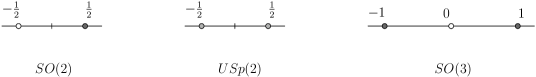
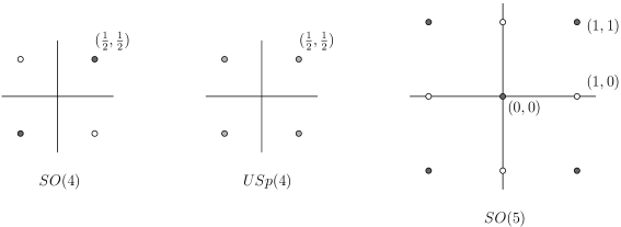
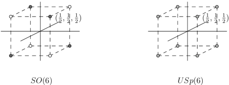
Figure 1: The special points for the $k=1$ vortex.

5 Fractional vortices and lumps

Another exciting recent result concerns the fractional vortex and lumps.[18] We have pointed out above that in a general class of gauge theories the vacuum is not unique, even if the Fayet-Iliopoulos term is present and even if the number of the flavors is the minimum possible for a “color-flavor” locked vacuum to exist. In other words, there is a nontrivial vacuum degeneracy, or the vacuum moduli ${\cal M}$. In the first part of the talk, we were mainly interested in the vortex moduli ${\cal V}$, in a particular, maximally color-flavor locked vacuum. Here we are going to consider all possible vortices—the vortex moduli ${\cal V}$—on all possible points of the vacuum moduli ${\cal M}$ at the same time.

There are in fact two crucial ingredients for the fractional vortex: the vacuum degeneracy and the BPS saturated nature of the vortices. The first point was emphasized just above: the situation is schematically illustrated in Fig. 2. Even if we restrict ourselves to the minimally winding vortex solutions only, the vortices represent non-trivial fiber bundles over the vacuum moduli ${\cal M}$.

The BPS-saturated nature of the vortices, on the other hand, implies that the vortex equations are reduced to the first-order equations. The matter equations of motion are solved by the moduli-matrix Ansatz. The other equations–the gauge field equations–reduce, in the strong coupling limit or, anyway, sufficiently far from the vortex center, to the vacuum equations for the scalar fields. In other words, the vortex solutions approximate the sigma model lumps.

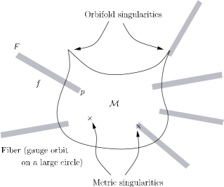
Figure 2: Vacuum moduli ${\cal M}$, fiber $F$ over it, and possible singularities

5.1 Structures of the vacuum moduli

Let $M$ be the manifold of the minima of the scalar potential, the vacuum configuration $M=\{q_{i}\ |\ q^{\dagger}T^{I}q=\xi^{I}\}$. The vacuum moduli ${\cal M}$ is given by the points

$$p\in{\cal M}=M/F\ ,$$ (26)

where the fiber $F$ is the sum of the gauge orbits of a point in $M$. A vortex solution is defined on each point of ${\cal M}$, in the sense that the scalar configuration along a sufficiently large circle ($S^{1}$) surrounding it traces a non-trivial closed orbit in the fiber $F$ (hence a point in ${\cal M}$). The existence of a vortex solution requires that

$$\pi_{1}\left(F,f\right)\neq\mathbf{1}\ ,$$ (27)

where $f$ is a point in $M$. The field configuration on a disk $D^{2}$ encircled by $S^{1}$ traces ${\cal M}$, apart from points at finite radius where it goes off $M$ (hence from ${\cal M}$). In other words it represents an element of $\pi_{2}({\cal M},p)$, where $p$ is the gauge orbit containing $f$, or $p=\pi(f)$: $\pi$ is the projection of the fiber onto a point of the base space ${\cal M}$. The exact sequence of homotopy groups for the fiber bundle reads

$$\cdots\to\pi_{2}\left(M,f\right)\to\pi_{2}\left({\cal M},p\right)\to\pi_{1}\left(F,f\right)\to\pi_{1}\left(M,f\right)\to\pi_{1}\left({\cal M},p\right)\to\cdots$$

where $\pi_{2}(M/F,f)\sim\pi_{2}({\cal M},p)$. See Fig. 3.

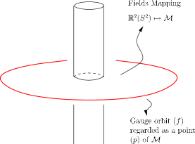
Figure 3:

Given the points $f,p$ and the space ${\cal M}$, the vortex solution is still not unique. Any exact symmetry of the system broken by an individual vortex solution gives rise to vortex zero modes (moduli), $\cal{V}$. Our main interest here however is the vortex moduli which arises from the non-trivial vacuum moduli ${\cal M}$ itself. Due to the BPS nature of our vortices, the gauge field equation

$$F_{12}^{I}=g_{I}^{2}\left(q^{{\dagger}}T^{I}q-\xi^{I}\right)\ ,$$

reduces, in the strong-coupling limit (or in any case, sufficiently far from the vortex center), to the vacuum equation defining $M$. This means that a vortex configuration can be approximately seen as a non-linear $\sigma$-model (NL$\sigma$M) lump with target space ${\cal M}$, as was already anticipated. Various distinct maps $S^{2}\mapsto{\cal M}$ of the same homotopy class correspond to physically inequivalent solutions; each of these corresponds to a vortex with the equal tension

$$T_{\rm min}=-\xi^{I}\int d^{2}x\,F_{12}^{I}>0\ ,$$

by their BPS nature. They represent non-trivial vortex moduli.

The semi-local vortices of the so-called extended-Abelian Higgs (EAH) model arise precisely this way. In an Abelian Higgs model with $N$ flavors of (scalar) electrons, $M=S^{2N-1}$, $F=S^{1}$, ${\cal M}=S^{2N-1}/S=\mathbb{C}P^{N-1}$, and the exact homotopy sequence tells us that $\pi_{2}(\mathbb{C}P^{N-1})$ and $\pi_{1}(S^{1})$ are isomorphic: each (i.e. minimum) vortex solution corresponds to a minimal $\sigma$-model lump solution.

In most cases discussed in our paper [18], however, the base space ${\cal M}$ will be various kinds of singular manifolds: a manifold with singularities, unlike in the EAH model. The nature of the singularities depends on the system and on the particular point(s) of ${\cal M}$. Our BPS degenerate vortices represent (generalized) fiber bundles with the singular manifolds ${\cal M}$ as the base space.

5.2 Two mechanisms for fractional vortex–lump

There are two distinct mechanisms leading to the appearance of a fractional vortex. The first is related to the presence of orbifold singularities in ${\cal M}$. For example, let us consider a ${\mathbbm{Z}}_{2}$ point $p_{0}$ such as the one appearing in a simple $U(1)$ model with two scalars, one of which has charge $2$. At this singularity, both $\pi_{2}\left({\cal M},p\right)$ and $\pi_{1}\left(F,f\right)$ make a discontinuous change. The minimum element of $\pi_{1}\left(F_{0},f_{0}\right)$ is half of that of $\pi_{1}\left(F,f\right)$ defined off the singularity, and similarly for $\pi_{2}\left({\cal M},p_{0}\right)$ with respect to $\pi_{2}\left({\cal M},p\right)$, $p\neq p_{0}$. Even though the exact homotopy sequence continues to hold on and off the orbifold point, the vortex defined near such a point will look like a doubly-wound vortex, with two centers (if the vortex moduli parameters are chosen appropriately). Analogous multi-peak vortex solution occurs near a ${\mathbbm{Z}}_{N}$ orbifold point of ${\cal M}$.

Another cause for the appearance of fractional peaks is simple and very general: a deformed sigma model geometry. This phenomenon can be best seen by considering our system in the strong coupling limit. Even if the base point $p$ is a perfectly generic, regular point of ${\cal M}$, not close to any singularity, the field configurations in the transverse plane ($S^{2}$) trace the whole vacuum moduli space ${\cal M}$. The energy distribution reflects the nontrivial structure of $\cal{M}$ as the volume of the target space is mapped into the transverse plane, $\mathbb{C}$

$$E=2\int_{\mathbb{C}}\frac{\partial^{2}K}{\partial\phi^{I}\partial\phi^{{\dagger}\bar{J}}}\partial\phi^{I}\bar{\partial}\phi^{{\dagger}\bar{J}}=2\int_{\mathbb{C}}\bar{\partial}\partial K\ .$$

The field configuration may hit for instance one of the singularities (conic or not), or simply the regions of large scalar curvature. Such phenomena thus occur very generally if the underlying sigma model has a deformed geometry . At such points the energy density will show a peak, not necessarily at the vortex center. Even at finite coupling, the vortex tension density will exhibit a similar substructure.

5.3 Some models

A simple model showing the fractional vortex is an extended Abelian Higgs model, with two scalar fields $A$ and $B$ with charges $2$ and $1$, respectively. Depending on the point of ${\cal M}$ (which is $\mathbb{C}P^{1}$) the minimum vortex shows doubly-peaked substructure clearly, see Fig. 4. The fractional vortex structure in this model nicely illustrates the first mechanism discussed above: the point $B=0$ is a $Z_{2}$ orbifold point, since there the only nonvanishing field, $A$, having charge $2$, must wind only half of the $U(1)$ to be single-valued.

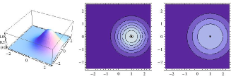
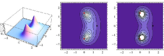
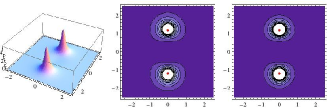
Figure 4: The energy (the left-most and the 2nd left panels) and the magnetic flux (the 2nd right panels) density, together with the boundary values $(A,B)$ (the right-most panel) for the minimal vortex.

Another interesting model is a $U_{1}(1)\times U_{2}(1)$ gauge theory with three flavors of scalar electrons $H=(A,B,C)$ with charges $Q_{1}=(2,1,1)$ for $U(1)_{1}$ and $Q_{2}=(0,1,-1)$ for $U(1)_{2}$. Even though the model has the same $\mathbb{C}P^{1}$ as the vacuum moduli ${\cal M}$ as the first model, the vortex properties are quite different. This model turns out to provide a good example of fractional vortex of the second type (deformed sigma-model geometry).

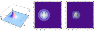
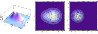
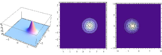
Figure 5: The energy density (left-most) and the magnetic flux density $F_{12}^{(1)}$ (2nd from the left), $F_{12}^{(1)}$ (2nd from the right) and the boundary condition (right-most).

Fractional vortex occurs also in non-Abelian gauge theories, such as the one with gauge group $G=SO(N)\times U(1)$. An illustrative example of fractional vortex in an $SO(6)\times U(1)$ model is shown in Fig. 6.

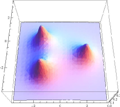
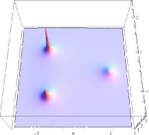
Figure 6: The energy density of three fractional vortices (lumps) in the $U(1)\times SO(6)$ model in the strong coupling approximation. The positions are $z_{1}=-\sqrt{2}+i\sqrt{2},z_{2}=-\sqrt{2}-i\sqrt{2},z_{3}=2$. The two figures correspond to two different choices of certain size moduli parameters.

6 Why non-Abelian vortices imply non-Abelian monopoles

A more recent work of our research group concerns the monopole-vortex complex solitons occurring in systems with hierarchical gauge symmetry breaking,

$$G\,\,\,{\stackrel{{\scriptstyle\langle\phi_{1}\rangle\neq 0}}{{\longrightarrow}}}\,\,\,H\,\,\,{\stackrel{{\scriptstyle\langle\phi_{2}\rangle\neq 0}}{{\longrightarrow}}}\,\,\,{\mathbbm{1}}\;,\qquad|\langle\phi_{1}\rangle|\gg|\langle\phi_{2}\rangle|\;.$$ (28)

The homotopy-group sequence

$$\cdots\to\pi_{2}(G)\to\pi_{2}(G/H)\to\pi_{1}(H)\to\pi_{1}(G)\to\cdots\,.$$ (29)

tells us that the properties of the regular monopoles arising from the breaking $G\to H$ are related to the vortices of the low-energy system. In particular, the fact that $\pi_{2}(G)={\mathbbm{1}}$ for any group $G$, implies that

$$\pi_{2}(G/H)\sim\pi_{1}(H)/\pi_{1}(G)\;.$$ (30)

For instance, in the case of the symmetry breaking, $SU(N+1)\to SU(N)\times U(1)/{\mathbbm{Z}}_{N}$ the first set of checks (on the Abelian and non-Abelian magnetic flux matching) have been done [20] soon after the discovery of the non-Abelian vortex in the $U(N)$ theory. We wish to study more carefully the monopole-vortex configurations, taking into account a small non-BPS correction term.

For instance one might study the model based on hierarchically broken gauge symmetry, $SU(3)\to SU(2)\times U(1)\to{\mathbbm{1}}$, with the Hamiltonian,

$$H = \int d^{3}x\Big{[}\,\frac{1}{4g^{2}}(F_{ij}^{3})^{2}+\frac{1}{4g_{0}^{2}}(F_{ij}^{0})^{2}+\frac{1}{g^{2}}|{\cal D}_{i}\phi^{a}|^{2}+\frac{1}{g_{0}^{2}}|{\cal D}_{i}\phi^{0}|^{2}+|{\cal D}_{i}q|^{2}$$

$$+ g_{0}^{2}|\mu\phi^{8}+{\sqrt{2}}Q^{\dagger}t^{8}Q|^{2}+g^{2}|\mu\phi^{3}+{\sqrt{2}}Q^{\dagger}t^{3}Q|^{2}+2\,Q^{\dagger}\lambda^{\dagger}\lambda Q\,\Big{]}\;.$$

describing the system after the first breaking. Such a low-energy theory is of the type studied in our original work on non-Abelian vortex [8], except for small terms involving $\phi^{3}(x)$ and $\phi^{8}(x)$ (which were set to their constant VEV in that paper). In fact, the model is the same as the one studied by Auzzi et. al. recently [21]. The system has unbroken, exact color-flavor diagonal $SU(2)_{C+F}$ symmetry. Neglecting the fields which get mass of the order of the higher symmetry breaking scale, and the fields which go to zero exponentially outside the monopole size, one makes an Ansatz (in the monopole and vortex singular gauge):

$$A_{\phi}=t_{3}A_{\phi}^{3}(\rho,z)+t_{8}A_{\phi}^{8}(\rho,z);\qquad A_{\phi}^{3}=-\frac{1}{\rho}f_{3}(\rho,z),\quad A_{\phi}^{8}=-\sqrt{3}\frac{1}{\rho}f_{8}(\rho,z),$$

$$\phi({\bf r})=\left(\begin{array}[]{ccc}v&0&0\\ 0&v&0\\ 0&0&-2v\end{array}\right)+\lambda(\rho,z),\qquad\lambda(\rho,z)=t_{3}\lambda_{3}(\rho,z)+t_{8}\lambda_{8}(\rho,z)\;.$$

$$q(x)=\left(\begin{array}[]{cc}w_{1}(\rho,z)&0\\ 0&w_{2}(\rho,z)\\ \end{array}\right)\;,$$

with appropriate boundary conditions. The equations for the profile functions $f_{3},f_{8},w_{1}w_{2},\lambda_{3},\lambda_{8}$ may be studied numerically. Some qualitative features can be read off from the structure of these equations.

(i)

The Dirac string of the monopole is hidden deep in the vortex core; the zero of the squark field at the vortex core makes the singularity harmless.

(ii)

The whole monopole-vortex complex breaks $SU(2)_{C+F}$: the orientational zeromodes develops which live on $SU(2)/U(1)\sim CP^{1}$.

(iii)

The degeneracy between the monopole of the broken “$U$ spin” and the monopole of the broken “$V$-spin”, which are naïvely related by the unbroken $SU(2)$ of the high-mass-scale breaking $SU(3)\to SU(2)\times U(1)$, is explicitly broken in the vacuum with small squark VEV.

(iv)

Nevertheless, there is a new, exact continuous degeneracy among the monopole-vortex complex configurations, related by the color-flavor symmetry ($CP^{1}$ moduli). It is possible that such an exact non-Abelian symmetry possessed by the monopole is at the origin of the non-Abelian dual gauge symmetry which emerges at low energies of the softly broken ${\cal N}=2$ supersymmetric QCD [6].

References

- [1] G. ’t Hooft, Nucl. Phys. B 79, 817 (1974), A.M. Polyakov, JETP Lett. 20, 194 (1974).
- [2] A. Abrikosov, Sov. Phys. JETP 32, 1442 (1957); H. Nielsen, P. Olesen, Nucl. Phys. B 61, 45 (1973).
- [3] N. Seiberg, E. Witten, Nucl. Phys. B 426, 19 (1994); Erratum ibid. B 430, 485 (1994).
- [4] N. Seiberg, E. Witten, Nucl. Phys. B 431, 484 (1994).
- [5] P. C. Argyres, M. R. Plesser, N. Seiberg, Nucl. Phys. B 471, 159 (1996); P.C. Argyres, M.R. Plesser, A.D. Shapere, Nucl. Phys. B 483, 172 (1997); K. Hori, H. Ooguri, Y. Oz, Adv. Theor. Math. Phys. 1, 1 (1998).
- [6] G. Carlino, K. Konishi, H. Murayama, JHEP 0002, 004 (2000); Nucl. Phys. B 590, 37 (2000).
- [7] A. Hanany and D. Tong, JHEP 0307, 037 (2003) [arXiv:hep-th/0306150].
- [8] R. Auzzi, S. Bolognesi, J. Evslin, K. Konishi and A. Yung, Nucl. Phys. B 673, 187 (2003) [arXiv:hep-th/0307287].
- [9] D. Tong, “TASI lectures on solitons,” arXiv:hep-th/0509216.
- [10] M. Shifman and A. Yung, Rev. Mod. Phys. 79, 1139 (2007), [arXiv:hep-th/0703267].
- [11] M. Eto, Y. Isozumi, M. Nitta, K. Ohashi and N. Sakai, J. Phys. A 39, R315 (2006), [arXiv:hep-th/0602170].
- [12] P. Goddard, J. Nuyts and D. Olive, Nucl. Phys. B 125 (1977) 1; F. A. Bais, Phys. Rev. D 18 (1978) 1206; B. J. Schroers and F. A. Bais, Nucl. Phys. B 512 (1998) 250, hep-th/9708004; Nucl. Phys. B 535 (1998) 197, hep-th/9805163; E. J. Weinberg, Nucl. Phys. B 167 (1980) 500; Nucl. Phys. B 203 (1982) 445.
- [13] K. Konishi and L. Spanu, Int. J. Mod. Phys. A18 (2003) 249, arXiv: hep-th/0106175.
- [14] A. Abouelsaood, Nucl. Phys. B 226, 309 (1983); P. Nelson, A. Manohar, Phys. Rev. Lett. 50, 943 (1983); A. Balachandran, G. Marmo, M. Mukunda, J. Nilsson, E. Sudarshan, F. Zaccaria, Phys. Rev. Lett. 50, 1553 (1983); P. Nelson, S. Coleman, Nucl. Phys. B 227, 1 (1984)
- [15] N. Dorey, C. Fraser, T.J. Hollowood, M.A.C. Kneipp, “NonAbelian duality in N=4 supersymmetric gauge theories,” [arXiv: hep-th/9512116]; Phys.Lett. B 383, 422 (1996)
- [16] M. Eto, L. Ferretti, K. Konishi, G. Marmorini, M. Nitta, K. Ohashi, W. Vinci, N. Yokoi, Nucl.Phys. B780, 161-187 (2007), [arXiv: hep-th/0611313].
- [17] M. Eto, T. Fujimori, S. B. Gudnason, K. Konishi, T. Nagashima, M. Nitta, K. Ohashi, W. Vinci, JHEP 0906:004 (2009), arXiv:0903.4471 [hep-th]; M. Eto, T. Fujimori, S. B. Gudnason, K. Konishi, M. Nitta, K. Ohashi, W. Vinci, Phys. Lett. B669: 98-101 (2008), arXiv:0802.1020 [hep-th].
- [18] M. Eto, T. Fujimori, S. B. Gudnason, K. Konishi, T. Nagashima, M. Nitta, K. Ohashi, W. Vinci, Phys. Rev. D80:045018,2009, arXiv:0905.3540 [hep-th].
- [19] B. Collie, D. Tong, JHEP 0908:006,2009, e-Print: arXiv:0905.2267 [hep-th].
- [20] R. Auzzi, S. Bolognesi, J. Evslin and K. Konishi, Nucl. Phys. B 686, 119 (2004), [arXiv:hep-th/0312233].
- [21] R. Auzzi, M. Eto, W. Vinci, JHEP 0711:090,2007, arXiv:0709.1910 [hep-th].