On the background in the $\gamma p\to\omega(\pi^{0}\gamma)p$ reaction
and mixed event simulation

Abstract

In this paper we evaluate sources of background for the $\gamma p\to\omega p$, with the $\omega$ detected through its $\pi^{0}\gamma$ decay channel, to compare with the experiment carried out at ELSA. We find background from $\gamma p\to\pi^{0}\pi^{0}p$ followed by decay of a $\pi^{0}$ into two $\gamma$, recombining one $\pi^{0}$ and one $\gamma$, and from the $\gamma p\to\pi^{0}\eta p$ reaction with subsequent decay of the $\eta$ into two photons. This background accounts for the data at $\pi^{0}\gamma$ invariant masses beyond 700 MeV, but strength is missing at lower invariant masses which was attributed to photon misidentification events, which we simulate to get a good reproduction of the experimental background. Once this is done, we perform an event mixing simulation to reproduce the calculated background and we find that the method provides a good description of the background at low $\pi^{0}\gamma$ invariant masses but fakes the background at high invariant masses, making background events at low invariant masses, which are due to $\gamma$ misidentification events, responsible for the background at high invariant masses which is due to the $\gamma p\to\pi^{0}\pi^{0}p$ and $\gamma p\to\pi^{0}\eta p$ reactions.

1 Introduction

The interaction of vector mesons with nuclear matter has attracted attention for a long time and has been tied to fundamental aspects of QCD. Yet, the theoretical models offer a large variety of results from a large attraction to a large repulsion. Early results on this issue within the Nambu Jona Lasinio model produced no shift of the masses Bernard:1988db while, using qualitative arguments, a universal large shift of the mass was suggested in Brown:1991kk . More recent detailed calculations show no shift of the mass of the $\rho$ meson in matter Rapp:1997fs ; Urban:1999im ; Cabrera:2000dx . Experimentally the situation has undergone big steps recently with the NA60 collaboration reporting a null shift of the $\rho$ mass in the medium Arnaldi:2006jq ; Damjanovic:2007qm in the dilepton spectra of heavy ion reactions and also a null shift in the $\gamma$ induced dilepton production at CLASS Wood:2008ee . On the other hand the KEK team had earlier reported an attractive mass shift of the $\rho$ in Muto:2005za ; Naruki:2005kd . As explained in detail in Wood:2008ee , the different conclusions can be traced back to the way the background is subtracted. Thus, the treatment of the background is an essential part of the investigation of the vector meson properties in nuclei. The case of the $\omega$ in the medium is more obscure. Theoretically there are about twenty different works with claims from large attraction to large repulsion (see Muhlich:2003tj ; Kaskulov:2006zc ; Kaskulov:2006fi for details). Experimentally there are claims of a large shift of the mass of the $\omega$ from the study of the photon induced $\omega$ production in nuclei, with the $\omega$ detected through its $\pi^{0}\gamma$ decay channel david ; prl . However, it was shown in Kaskulov:2006zc that the shift could just be a consequence of a particular choice of background subtraction and that other reasonable choices led to different conclusions. For instance, choosing a background in the nuclear case proportional to the background on the proton in the region below the $\omega$ peak, the experimental data could be explained without a shift of the $\omega$ mass in the medium.

The method to determine the mass shift is very different from the one used to determine the width in the medium. This latter one relies upon the production cross section in different nuclei, which leads to the transparency ratio that allows to determine a large width of the $\omega$ in the medium Kaskulov:2006zc ; :2008xy . By contrast the measurement of the mass requires the analysis of the shape of the invariant mass distribution, which is barely affected in nuclei because practically all $\omega$ decays occur in the nuclear surface or outside the nucleus.

The discussion on the issue of the $\omega$ mass shift was followed by the evaluation of the background with the mixed event technique in metagerice . There the background for a nuclear target was evaluated and found to be the same as assumed in prl , and again it was concluded that the data demanded a shift of the $\omega$ mass in the medium.

The former discussion indicates that the treatment of background is an essential issue in this problem. In view of this we decided to face the problem and investigate the details on how the mixed event technique works in the present case. For this we followed the strategy of evaluating the background for the proton target. We could trace two sources of background that account for the experimental cross section at $\pi^{0}\gamma$ invariant masses of the order of the $\omega$ mass and beyond. The rest of the background at lower invariant masses was simulated to account for $\gamma$ misidentification events, as found in david . Once a background consistent with the experiment is obtained theoretically, we apply the mixed event technique to obtain the background and compare it with the theoretical one. In this way we can determine the ability of the mixed event method to reproduce the background in this reaction. The results that we find are that the method can provide the background at low invariant masses, where the cross sections are large, but it actually fakes the background in the region of invariant masses around and beyond the $\omega$ mass. We show that the mixed event generated background in that region is completely tied to the real events at low $\pi^{0}\gamma$ invariant masses where the $d\sigma/dM_{\pi^{0}\gamma}$ distribution is larger. As a result, we show that the distribution obtained with the mixed event method in the region of invariant masses around and beyond the $\omega$ mass is largely insensitive to the actual background contributing in that region. But this is precisely the region where the background is needed to determine changes of the $\omega$ signal in the nuclear medium. As a consequence we clearly show that the mixed event technique is unsuited in the present case as an instrument to determine possible shifts of the $\omega$ mass in the medium.

In the meantime, a recent reanalysis of the background of the reaction of david ; prl done in marianahad concludes, however, that one cannot claim a shift of the $\omega$ mass from this experiment.

2 Background sources in the reaction $\gamma p\to\omega p\ (\omega\to\pi^{0}\gamma)$

The reaction that we study is $\gamma p\to\omega p$ where the $\omega$ is detected through its $\omega\to\pi^{0}\gamma$ decay mode. This is the reaction studied in the CBELSA/TAPS experiment. According to the study in david , in the region of the reconstructed invariant mass of the $\pi^{0}\gamma$ one of the main sources of background comes from the $\gamma p\to\pi^{0}\pi^{0}p$ reaction followed by the decay of any of the two $\pi^{0}$ into $\gamma\gamma$. Then, background events appear from the combination of one of these photons and the remaining $\pi^{0}$. Another source is the $\gamma p\to\pi^{0}\eta p$ reaction. We evaluate the cross section for those two processes in the following subsection.

2.1 The $\gamma p\to\pi^{0}\pi^{0}p$ reaction

This reaction has been thoroughly studied at Mainz Braghieri:1994rf ; Harter:1997jq ; mainz ; Schadmand:2005ji and more recently at ElSA elsa ; thoma , GRAAL Ajaka:2007zz and Jefferson Lab Ripani:2000aw ; jeff ; Burkert:2007kn . We are interested not only in the cross section for the reaction but at the same time to have an event generator that provides events weighed by their probability determined by the available phase space. For this purpose the Monte Carlo evaluation of the cross section integral is the most suited algorithm since it provides the events allowed by phase space properly weighted and the cross section in the end.

The $\gamma p\to\pi^{0}\pi^{0}p$ cross section is given by

$$\sigma=\frac{M^{2}_{N}}{s-M^{2}_{N}}\int\frac{d^{3}p_{1}}{(2\pi)^{3}}\int\frac{d^{3}p_{2}}{(2\pi)^{3}}\int\frac{d^{3}p_{3}}{(2\pi)^{3}}$$

$$\times\frac{1}{2E(p_{1})}\frac{1}{2E(p_{2})}\frac{1}{2E(p_{3})}\left|T\right|^{2}$$

$$\times(2\pi)^{4}\delta(p_{\gamma}+p_{p}-p_{1}-p_{2}-p_{3}),$$ (1)

which includes the 1/2 symmetry factor to account for the two identical pions in the final state. The variables $p_{1},\,p_{2},\,p_{3}$ are the momenta of the final proton and the two $\pi^{0}$ respectively and $T$ stands for the transition matrix for the $\gamma p\to\pi^{0}\pi^{0}p$ process. In the $\left|T\right|^{2}$ factor a sum over final spins and a proper average over initial spins is implicit.

Since $d^{3}p/E(p)$ is a Lorentz invariant measure, we proceed to evaluate the last two integrals in Eq. (1) in the reference frame where $\vec{p}_{\gamma}+\vec{p}_{p}-\vec{p}_{1}=\vec{0}$ which guarantees that $\vec{p}_{2}+\vec{p}_{3}=\vec{0}$. The cross section is then written as

$$\sigma=\frac{M^{2}_{N}}{s-M^{2}_{N}}\int\frac{d^{3}p_{1}}{(2\pi)^{3}}\frac{1}{2E(p_{1})}\theta(M_{23}-2m_{\pi^{0}})$$

$$\times\int d\Omega\ \tilde{p}_{2}\frac{1}{16\pi^{2}}\frac{1}{M_{23}}\left|T\right|^{2},$$ (2)

where $M_{23}$ is the invariant mass of the two $\pi^{0}$ given by

$$M_{23}^{2}=(p_{\gamma}+p_{p}-p_{1})^{2}=s+M^{2}_{N}-2(p_{\gamma}+p_{p})p_{1}.$$ (3)

We shall work in the laboratory (lab) frame that allows us to implement easily all the experimental cuts. The variable $\tilde{p}_{2}$ in Eq. (2) is the $\pi^{0}$ momentum in the $\pi^{0}\pi^{0}$ rest frame

$$\tilde{p}_{2}=\frac{\lambda^{\frac{1}{2}}(M_{23}^{2},m_{\pi^{0}}^{2},m_{\pi^{0}}^{2})}{2M_{23}},$$ (4)

and $d\Omega$ is performed in the $\pi^{0}\pi^{0}$ rest frame.

The $\gamma p\to\pi^{0}\pi^{0}p$ reaction has been studied theoretically at $E_{\gamma}<0.8$ GeV tejedor ; Bernard:1996ft ; roca ; nacher ; Ochi:1997ev and at higher energies $E_{\gamma}>1.5$ GeV in Ripani:2000aw ; Roberts:2004mn . We do not need any of these sophisticated models here. Our final goal is to see how much background comes form this source and to have an event generator by means of which we can study how the mixed event technique works in the present case. For this purpose it is enough to consider $|T|^{2}$ to be a constant over the phase space and fit its value to reproduce the experimental results for the cross section in the region of interest to us. We take the cross section for $\gamma p\to\pi^{0}\pi^{0}p$ at the needed photon energies from elsa ; thoma .

The next step is to write $\tilde{p}_{2}$ in the lab frame. We have in the $\pi^{0}\pi^{0}$ rest frame

$$\vec{\tilde{p}}_{2} = \tilde{p}_{2}\left\{\begin{array}[]{c}sin\theta\,cos\varphi\\ sin\theta\,sin\varphi\\ cos\theta\end{array}\right\}$$ (8)

$$\vec{\tilde{p}}_{3} = -\vec{\tilde{p}}_{2}$$ (9)

with $\theta,\varphi$ angles in the $\pi^{0}\pi^{0}$ rest frame. We then perform a boost of $\vec{\tilde{p}_{2}}$ to the lab frame where $\vec{p}_{2}+\vec{p}_{3}=\vec{p}_{\gamma}+\vec{p}_{p}-\vec{p}_{1}=\vec{P}$

$$\vec{p}_{2}=\left[\left(\frac{E_{23}}{M_{23}}-1\right)\frac{\vec{\tilde{p}}_{2}\cdot\vec{P}}{\vec{P}^{2}}+\frac{\tilde{p}_{2}^{0}}{M_{23}}\right]\vec{P}+\vec{\tilde{p}}_{2},$$ (10)

where $E_{23}$ is the two pion energy in the lab frame $E_{23}=(M_{23}^{2}+\vec{P}^{2})^{\frac{1}{2}}$. Similarly we boost $\vec{\tilde{p}}_{3}$ to $\vec{p}_{3}$ in the initial $\gamma p$ lab frame.

Assume now that the pion with momentum $\vec{p}_{2}$ is the one that decays into $\gamma\gamma$. In the pion rest frame the two $\gamma$’s will go back to back and one $\gamma$ will have the momentum

$$\vec{\tilde{p}}_{\gamma}=\frac{m_{\pi^{0}}}{2}\left\{\begin{array}[]{c}sin\theta_{\gamma}\,cos\varphi_{\gamma}\\ sin\theta_{\gamma}\,sin\varphi_{\gamma}\\ cos\theta_{\gamma}\end{array}\right\},$$ (14)

with $\theta_{\gamma},\,\varphi_{\gamma}$ angles of the photon in this one $\pi^{0}$ rest frame. Once again we boost this photon momentum to the frame where the pion has momentum $\vec{p}_{2}$

$$\vec{p}_{\gamma}=\left[\left(\frac{E_{2}}{m_{\pi^{0}}}-1\right)\frac{\vec{\tilde{p}}_{\gamma}\cdot\vec{p}_{2}}{\vec{p}_{2}^{2}}+\frac{\tilde{p}_{\gamma}^{0}}{m_{\pi^{0}}}\right]\vec{p}_{2}+\vec{\tilde{p}}_{\gamma}.$$ (15)

Since we can have a $\pi^{0}\gamma$ combination from either of the two $\pi^{0}$ or the two $\gamma$’s, we would obtain a combinatorial factor of four to account for these possibilities.

All this said, the cross section for $\gamma p\to\pi^{0}\pi^{0}p\to\gamma\gamma\ \pi^{0}p\to\gamma\pi^{0}+X$ reads

$$\sigma = 4\,\frac{M^{2}_{N}}{s-M^{2}_{N}}\int\frac{d^{3}p_{1}}{(2\pi)^{3}}\frac{1}{2E(p_{1})}\left|T\right|^{2}\theta(M_{23}-2m_{\pi^{0}})$$

$$\times \int_{-1}^{1}dcos\theta\int_{0}^{2\pi}d\varphi\,\tilde{p}_{2}\frac{1}{16\pi^{2}}\frac{1}{M_{23}}\frac{1}{4\pi}\int_{-1}^{1}dcos\theta_{\gamma}\int_{0}^{2\pi}d\varphi_{\gamma}$$

recalling from Eq. (3) that in the lab frame

$$M_{23}=s+M^{2}_{N}-2(E_{\gamma\,in}+M_{N})E(p_{1})+2\vec{p}_{\gamma\,in}\cdot\vec{p}_{1}$$ (17)

Next one generates random numbers for $\vec{p}_{1},\,\theta,\,\varphi,\,\theta_{\gamma},\,\varphi_{\gamma}$ with $|\vec{p}_{1}|$ restricted between zero and

$$|\vec{p}_{1}|^{max}_{lab}=\frac{|\vec{p}_{1}|^{max}_{CM}+v\,E_{1\,CM}^{max}}{\sqrt{1-v^{2}}}$$ (18)

with $|\vec{p}_{1}|^{max}_{CM}$ and $E_{1\,CM}^{max}$ the maximum momentum and energy allowed for the final proton in the $\gamma p$ center of mass (CM) frame, corresponding to the case when the two $\pi^{0}$ go together

$$|\vec{p}_{1}|^{max}_{CM}=\frac{\lambda^{\frac{1}{2}}(s,M^{2}_{N},4m_{\pi^{0}}^{2})}{2\sqrt{s}}$$ (19)

and $v$ is the velocity of the $\gamma p$ CM system measured in the lab frame

$$v=\frac{|\vec{p}_{\gamma\,in}|}{E_{\gamma\,in}+M_{N}}$$ (20)

For each of these events we evaluate the invariant mass

$$M_{inv}(\pi^{0}\gamma)=(p_{\gamma}+p_{3})^{2}$$ (21)

and store the events, properly weighted by $|T|^{2}$ and phase space factors, in boxes of $M_{inv}(\pi^{0}\gamma)$ for a suitable partition of $M_{inv}(\pi^{0}\gamma)$.

2.2 The $\gamma p\to\pi^{0}\eta p$ reaction

We also evaluate the background for the $\gamma p\to\pi^{0}\eta p$ reaction. In this case $\eta\to\gamma\gamma$ and we get one photon from there plus the $\pi^{0}$ to reconstruct the $\pi^{0}\gamma$ invariant mass. The changes with respect to the former reaction are minimal. Since now there is only one $\pi^{0}$, we do not have to include the 1/2 symmetry factor and the combinatorial factor of four before is now a factor of two and the mass of one pion must be changed to the mass of the $\eta$ when needed. There are data for this reaction in mariana ; Nakabayashi:2006ut ; Ajaka:2008zz ; ulrike . There are also recent detailed models for the reaction Doring:2005bx ; Doring:2006pt accounting fairly well for the cross section mariana ; Nakabayashi:2006ut and the asymmetries Ajaka:2008zz . However, once again, for the present problem it suffices to repeat the procedure done for the $\gamma p\to\pi^{0}\pi^{0}p$ reaction in the former section taking a constant $|T|^{2}$ and implementing properly the phase space demanding that we reproduce the data of mariana ; Nakabayashi:2006ut ; ulrike .

2.3 Background from extra sources

As we shall see in the results section, the $\gamma p\to\pi^{0}\pi^{0}p$ and $\gamma p\to\pi^{0}\eta p$ reactions can account for the background observed in the CBELSA/TAPS experiment david ; prl in the region of the $\omega$ excitation and higher $\pi^{0}\gamma$ invariant masses. However, it does not account for the large background observed in the region of $\pi^{0}\gamma$ invariant masses lower than $m_{\omega}$. Once again we resort to the findings of david suggesting that such events could come from reactions like $\gamma p\to\pi^{0}\pi^{+}n$ with a misidentification of the neutron by a photon and other possible sources of $\gamma$ misidentification. In this part we do not make a theory since the events come from ignorance of the occurring reactions and misidentification of particles which have to do with the detector system. However, we would like to have $\pi^{0}\gamma$ events corresponding to this region in order to perform later on the mixed event analysis.

To generate background events in this region we write the corresponding cross section as

$$\sigma = \int_{M_{inv}^{min}}^{M_{inv}^{max}}dM_{\pi\gamma}\ |T(M_{\pi\gamma})|^{2}$$

$$\times \int_{-1}^{1}dcos\theta\int_{0}^{2\pi}d\varphi\int d^{3}P_{CM}\ \theta(500\,{\rm MeV/c}-|\vec{P}_{CM}|)\ ,$$

where $|T(M_{\pi\gamma})|^{2}$ is a function to be determined from experiment. $\theta,\,\varphi$ are the $\pi^{0}$ angles in the $\pi^{0}\gamma$ rest frame. There the pion momentum is

$$\vec{\tilde{p}}_{\pi^{0}}=\tilde{p}_{\pi^{0}}\left\{\begin{array}[]{c}sin\theta\,cos\varphi\\ sin\theta\,sin\varphi\\ cos\theta\end{array}\right\},$$ (26)

with

$$\tilde{p}_{\pi^{0}}=\frac{M_{\pi\gamma}^{2}-m_{\pi^{0}}^{2}}{2M_{\pi\gamma}},~{}~{}~{}~{}~{}~{}~{}\vec{\tilde{p}}_{\gamma}=-\vec{\tilde{p}}_{\pi^{0}}.$$ (27)

Eq. (2.3) contains an integral over $\vec{P}_{CM}$ with a maximum of 500 MeV for $|\vec{P}_{CM}|$. This momentum represents the $\pi^{0}\gamma$ total momentum in the $\gamma_{in}p$ CM frame. In this frame the momenta are more evenly distributed than in the lab frame and then we take an isotropic distribution for $\vec{P}_{CM}$ with the constraint $|\vec{P}_{CM}|<500$ MeV/c. This is a conservative estimate that exceeds the phase space of Eq. (2.3) when $|\vec{P}|=|\vec{p}_{\pi^{0}}+\vec{p}_{\gamma}|$ the total $\pi^{0}\gamma$ momentum in the $\gamma_{in}p$ lab frame is restricted to values smaller than 500 MeV/c. Next we boost the $\pi^{0}$ and the $\gamma$ momenta from their CM frame to the $\gamma_{in}p$ CM frame where the $\pi^{0}\gamma$ system has momentum $\vec{P}_{CM}$. We have

$$\vec{p}^{\prime}_{\pi^{0}} = \left[\left(\frac{E_{\pi\gamma}}{M_{\pi\gamma}}-1\right)\frac{\vec{\tilde{p}}_{\pi^{0}}\cdot\vec{P}_{CM}}{\vec{P}^{2}_{CM}}+\frac{\tilde{p}_{\pi^{0}}^{0}}{M_{\pi\gamma}}\right]\vec{P}_{CM}+\vec{\tilde{p}}_{\pi^{0}},$$

$$E_{\pi\gamma} = \sqrt{\vec{P}^{2}_{CM}+M^{2}_{\pi\gamma}},$$ (29)

$$\vec{p}^{\prime}_{\gamma} = \vec{P}_{CM}-\vec{p}_{\pi^{0}}.$$ (30)

The next step is the boost to the lab system where the $\gamma_{in}p$ has momentum $\vec{p}_{\gamma\,in}$ and energy $E_{\gamma p}=p_{\gamma\,in}+M_{N}$, hence

$$\vec{p}_{\pi^{0}}=\left[\left(\frac{E_{\gamma p}}{\sqrt{s}}-1\right)\frac{\vec{p}^{\prime}_{\pi^{0}}\cdot\vec{p}_{\gamma\,in}}{\vec{p}^{2}_{\gamma\,in}}+\frac{p_{\pi^{0}}^{\prime\,0}}{\sqrt{s}}\right]\vec{p}_{\gamma\,in}+\vec{p}^{\prime}_{\pi^{0}},$$ (31)

and a similar one for $\vec{p}_{\gamma}$. On these $\gamma$ and $\pi^{0}$ momentum we enforce now the cut

$$\left|\vec{p}_{\pi^{0}}+\vec{p}_{\gamma}\right|<500\,{\rm MeV/c}.$$ (32)

The function $T(M_{\pi\gamma})$ of Eq. (2.3) is determined empirically such that the sum of the cross section for $\gamma p\to\pi^{0}\pi^{0}p$ plus $\gamma p\to\pi^{0}\eta p$, plus the new one simulating $\gamma$ misidentification events, gives the total experimental cross section of david ; prl .

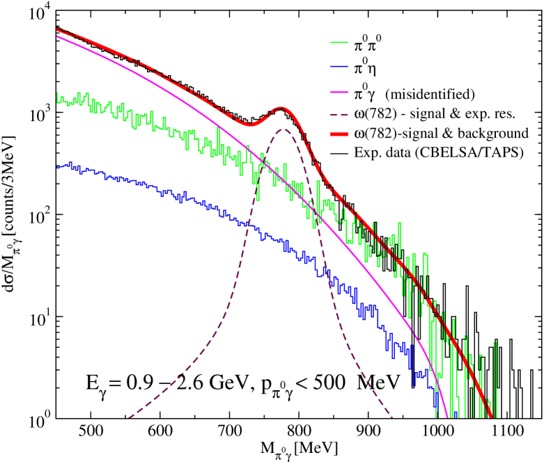
Figure 1: The invariant mass $d\sigma/dM_{\pi^{0}\gamma}$ distribution in the reaction $\gamma p\to\pi^{0}\gamma p$. The signal and different background contributions are also shown.

3 Mixed events calculation

In the mixed event simulation the idea is to obtain the background from the real data by evaluating $M_{\pi^{0}\gamma}$ selecting the $\pi^{0}$ and the $\gamma$ from two different events. The invariant mass distribution is then given by

$$M_{\pi^{0}\gamma}^{2}(ME)=(p_{\pi^{0}}(1)+p_{\gamma}(2))^{2}.$$ (33)

There is abundant literature on the subject  Drijard:1984pe ; Fachini:2002iz ; L'Hote:1992qz ; vanEijndhoven:2001kx ; Toia:2005vr and it has become a popular instrument to determine background and isolate particular reactions that peak at a certain place.

In our case where all the integrals of the cross sections are performed by Monte Carlo, the mixed event simulation is particularly simple to implement. The Monte Carlo integrals are done by generating random events into a volume $V$ containing the whole phase space and then the integral is given by the average value of the integrand, that we shall denote as $\widehat{|T|^{2}}$, times the volume

$$\sigma=\frac{\sum_{i=1}^{N}\widehat{|T_{i}|^{2}}}{N}\,V,$$ (34)

where one understand that $\widehat{|T_{i}|^{2}}$ is zero if the event generated does not belong to the phase space. Assume now that we take pair of events $i,j$ corresponding to a reaction channel. We have

$$\sigma^{2}=\frac{\sum_{i=1}^{N}\widehat{|T_{i}|^{2}}}{N}\,V\frac{\sum_{j=1}^{N}\widehat{|T_{j}|^{2}}}{N}\,V,$$ (35)

or equivalently

$$\sigma=\frac{1}{\sigma}\,\sum_{i=1}^{N}\sum_{j=1}^{N}\frac{\widehat{|T_{i}|^{2}}V\widehat{|T_{j}|^{2}}V}{N^{2}}.$$ (36)

We can then generate pairs of events in the phase space volume $V$ and the former integral gives the cross section. Simultaneously with the evaluation of the cross section we can obtain $M_{\pi^{0}\gamma}$ for each pairs of events as done in Eq. (33) and store the event, with its corresponding weight, in a box of a certain $M_{\pi^{0}\gamma}$ value. After the double sum in Eq. (36) we obtain the normalized $d\sigma/dM_{\pi^{0}\gamma}$ distribution.

The generalization to four channels as we have in our case, $\gamma p\to\pi^{0}\pi^{0}p$, $\gamma p\to\pi^{0}\eta p$, the channel from $\gamma$ misidentification and the $\gamma p\to\omega p\to\pi^{0}\gamma p$ channel is straightforward

$$\sigma_{tot}=\frac{1}{\sigma_{tot}}\,\sum_{\alpha}\sum_{\beta}\,\sum_{i=1}^{N}\sum_{j=1}^{N}\frac{\widehat{|T_{i,\alpha}^{(1)}|^{2}}V\widehat{|T_{j,\beta}^{(2)}|^{2}}V}{N^{2}},$$ (37)

where

$$\sigma_{tot}=\sigma_{1}+\sigma_{2}+\sigma_{3}+\sigma_{4},$$ (38)

and $\alpha,\beta$ run from 1 to 4. In order to obtain $d\sigma/dM_{\pi^{0}\gamma}$ from these mixed events we evaluate again $M_{\pi^{0}\gamma}$ from Eq. (33) and store the events in boxes of $M_{\pi^{0}\gamma}$ and we obtain at the end the histogram that provides us with the normalized $d\sigma/dM_{\pi^{0}\gamma}$ distribution from mixed events.

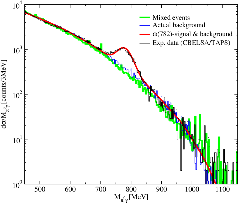
Figure 2: The mixed event background with method I is shown, together with the actual background, the results of the model for $\omega$ signal plus background and the data.

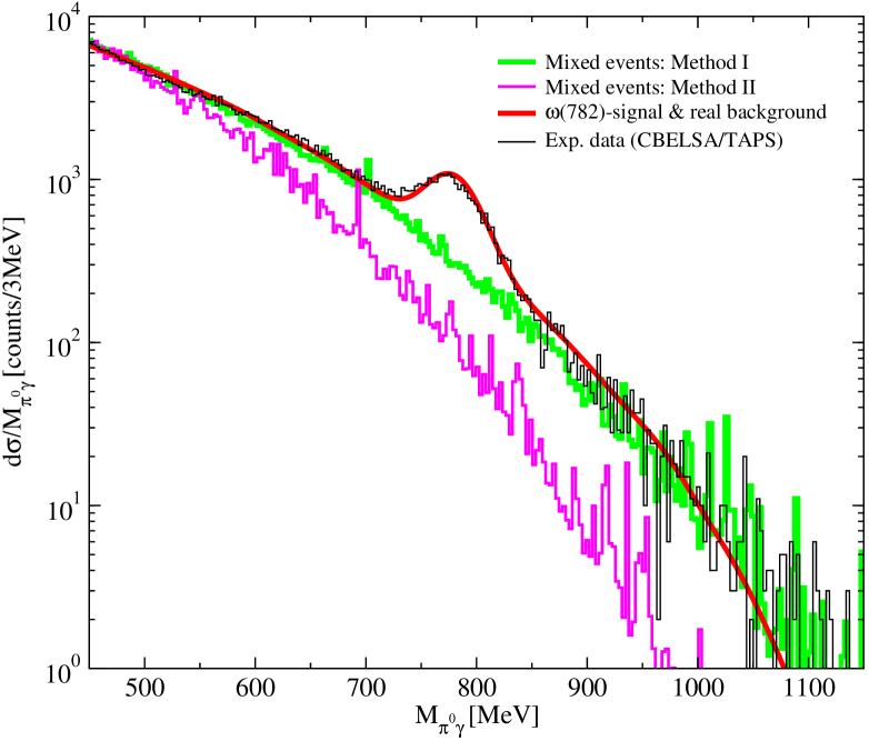
Figure 3: The effect of the momentum cut on the mixed events before and after the mixing (method II).

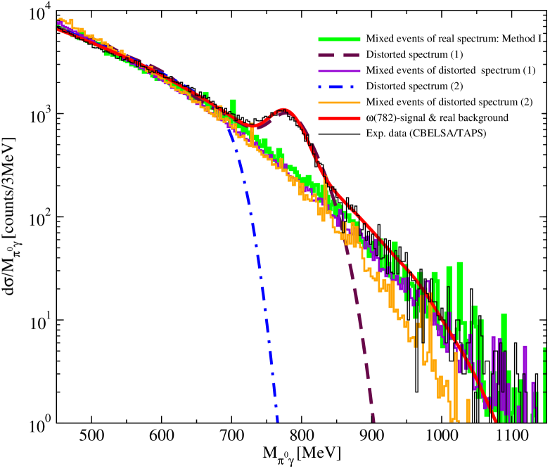
Figure 4: The mixed event background with Method I for different input invariant mass distributions.

4 Results

In Fig. 1 the contributions from the $\omega$-signal and different sources discussed above are compared with the experimental invariant mass $d\sigma/dM_{\pi^{0}\gamma}$ distribution in the reaction $\gamma p\to\pi^{0}\gamma p$ from CBELSA/TAPS experiment.

The sources of background are $\gamma p\to\pi^{0}\pi^{0}p$ with either of the two pions decaying into two $\gamma$, which was studied in section 2.1. This is the most important source of background in the region of the $\omega$ and beyond. The other important source of background is the $\gamma$ misidentification studied in Section 2.3. This source competes with the former one in the region of the omega and becomes dominant at smaller $\gamma\pi^{0}$ invariant masses. The third source considered is the one coming from $\gamma p\to\pi^{0}\eta p$ followed by the $\eta$ decay into two $\gamma$. This source has a smaller strength than the other two, but was found to be important to understand a peak in the experiment at lower $\gamma\pi^{0}$ invariant masses than the omega in Kaskulov:2006fi when protons were measured in coincidence. The omega signal comes from our study in Kaskulov:2006zc . The fit to the unnormalized data is done by adjusting the strength of the $\gamma p\to\pi^{0}\pi^{0}p$ source to the experiment distribution at large invariant mass, since this is the most important source in this invariant mass region. The source of the $\gamma p\to\pi^{0}\eta p$, as well as the signal are rescaled keeping their ratio, in order to keep the theoretical proportion between all these different sources. Finally, the source of misidentified $\gamma$ is added in order to complete a good description of the data. As one can see from the figure, the agreement of the theoretical model with the experimental data is very good. Note that we also have adapted our theoretical set up to the experimental one by choosing $E_{\gamma}=0.9-2.6~{}GeV$ and $p_{\pi^{0}\gamma}=|\vec{p}_{\pi^{0}}+\vec{p}_{\gamma}|\leq 500~{}MeV$.

We should note that the experimental spectrum shown in Fig. 1 is not acceptance corrected. The reason is that experimentally one observes only three out of four photons in the final state due to the detector inefficiencies, or the overlap of photon clusters, and the latter depends on the energy of the photon marianahad . Yet, in the unnormalized spectrum to which we make the fit, the differences are of the order of 20 % from the lower mass part of the spectrum to the higher mass one, and have irrelevant consequences for the argumentations and conclusions that follow. The consideration of acceptance would be more important in case one would like to compare our different sources of background with the acceptance uncorrected experimental determinations marianahad , which is not our concern here.

5 Mixed events and different tests

On the first hand we make the ME simulation that was done in metagerice taking two independent events and demanding that

$$|\vec{p}_{\pi^{0}}^{\,(1)}+\vec{p}_{\gamma}^{\,(2)}|<500\,{\rm MeV/c}$$ (39)

for the mixed event. We call it method I. This choice has in principle a conceptual flaw. Indeed, the curve in Fig. 1 corresponds to events in which one has imposed $|\vec{p}_{\pi^{0}}+\vec{p}_{\gamma}|<500$ MeV/c in the $\pi^{0}$ and $\gamma$ momenta of the same event. This restricts the phase space considerably. Now if one imposes Eq. (39) after the mixing, one can have both events (1) and (2) or one of them that do not fulfill separately $|\vec{p}_{\pi^{0}}+\vec{p}_{\gamma}|<500$ MeV/c and, as a consequence, these are events which do not contribute to the distribution of Fig. 1. In other words, one can be using events that do not provide any information to Fig. 1 to obtain its corresponding background through the mixed event method. Clearly in the extreme case that most events in the ME simulation do not pass the individual $|\vec{p}_{\pi^{0}}+\vec{p}_{\gamma}|<500$ MeV/c test one would be obtaining the background of the curve from a physical situation that has no relationship with the distribution of Fig. 1. How far is one in practice from this situation depends of course on the cut.

In Fig. 2 we show the results that we get from the mixed event simulation for the background, compared to the real background of the theoretical model. We can see that there is a remarkable agreement between the two in the whole range of invariant masses. We might conclude from there that the mixed event method is really good to reproduce the background. Yet, let us investigate with more detail how this shape has been produced. Upon renormalization of the generated mixed event distribution we reproduce the real background, but we know that one is using for sure information not included in the spectrum of Fig. 1.

Another way to proceed is to select two independent events from Fig. 1, meaning that each one separately fulfills $|\vec{p}_{\pi^{0}}+\vec{p}_{\gamma}|<500$ MeV/c, and then reconstruct the invariant mass of Eq. (33) for the mixed events, imposing also the cut of Eq. (39) to the pair of events of the mixing. We call that method II. This would correspond to a ME reconstruction from experimental events that have been filtered with the $|\vec{p}_{\pi^{0}}+\vec{p}_{\gamma}|<500$  MeV/c condition, which imposes a certain correlation, which might be undesired, in the events chosen for the mixing. The results can be seen in Fig. 3. Now we normalize the background at low invariant masses where it is maximum. Then we observe that in the rest of the invariant mass region there is a clear disagreement of this new mixed events background with the real one. Hence, the result has been a very poor reproduction of the real background by the mixed event method II.

Going back to method I, and in order to understand what is really happening, we have conducted another test. Let us realize that the mass distribution of Fig. 1 is exponential and there are three orders of magnitude difference between the strength of $d\sigma/dM_{\pi^{0}\gamma}$ at low and large invariant masses. From pure statistics it looks quite logical that if we take two independent events to reconstruct the mixed event $\pi^{0}\gamma$ invariant mass, these two events belong to the region of the spectrum that has larger cross section, even if the mass that we obtain corresponds to the large invariant mass where $d\sigma/dM_{\pi^{0}\gamma}$ is small. In other words, it is perfectly acceptable that the background that one obtains in the large invariant mass region is largely determined by events far away from this region, sitting at much lower individual $\pi^{0}\gamma$ invariant masses. If this were the case one would be attributing the background in the high invariant mass region to different reactions than those responsible for it and hence one would be distorting the physics of the process. Certainly in such a case there would be an interesting side effect: the distribution obtained with the mixed event method at large invariant masses would be largely insensitive to the actual background contributing in that region. In this case the ME method would thus render a background in this region that has nothing to do with the actual one.

In order to illustrate more dramatically the problem, we change arbitrarily the background of our model at large $M_{\pi^{0}\gamma}$ by imposing

$$|T|^{2}\to|T|^{2}\ f(M_{\pi^{0}\gamma})$$ (40)

where $f(M_{\pi^{0}\gamma})$ is a distortion factor. We consider two sharp cuts with

$$(1)~{}~{}f(M_{\pi^{0}\gamma})=\left\{\begin{array}[]{ll}1&{\rm\ \ \ for}\ M_{\pi^{0}\gamma}<850\,{\rm MeV}\\ 0&{\rm\ \ \ for}\ M_{\pi^{0}\gamma}>850\,{\rm MeV}\end{array}\right.$$ (43)

and

$$(2)~{}~{}f(M_{\pi^{0}\gamma})=\left\{\begin{array}[]{ll}1&{\rm\ \ \ for}\ M_{\pi^{0}\gamma}<750\,{\rm MeV}\\ 0&{\rm\ \ \ for}\ M_{\pi^{0}\gamma}>750\,{\rm MeV}\end{array}\right.$$ (46)

The distortion factor in Eq. (43) cuts off the background at higher invariant masses beyond the $\omega$-signal and (46) removes both the signal and the background.

In Fig. 4 we show the results for the background from the ME method, with method I and the real data, compared with those obtained with the distorted spectra of Eqs. (43) and (46). Note that the sharp cut off becomes in the figure a smoother fall down because we implement the folding of the $\pi^{0}\gamma$ invariant mass with the experimental resolution of prl of $50~{}MeV$. What we see in Fig. 4 is that the ME method output barely changes with the actual background from Eqs. (43,46), or in other words, that the ME method is unable to produce the actual background. It produces a background largely tied to the events at low invariant mass and is unsuited to produce a realistic background in the region of large $M_{\pi^{0}\gamma}$ masses.

In order to test the former suggestion that the background at large invariant masses in the ME method is tied to events at low invariant masses, we construct the correlation matrix $C(M_{\pi\gamma}(ini),M_{\pi\gamma}(fin))$ where $M_{\pi\gamma}(ini)$ refers to any of the two events used in the mixed event simulation and $M_{\pi\gamma}(fin)$ refers to the ME final invariant mass determined through Eq. (33).

In Fig. 5 we plot the correlation function. We have taken $M_{\pi\gamma}(fin)=800~{}MeV$. Then keeping this variable fixed we plot on the y-axis in an arbitrary scale the number of events (summing the two events used in the mixing) that would have a certain $M_{\pi\gamma}(ini)$. As we can see, the initial events used in the mixing accumulate in the region where $M_{\pi\gamma}(ini)$ is about 400-500 MeV. This certainly is distorting the physics of the problem, since the background associated to the region $M_{\pi\gamma}(fin)=800~{}MeV$ is generated after mixing by events around 400 MeV, where the origin of the background is quite different from the real one around $M_{\pi\gamma}(fin)=800~{}MeV$.

6 Summary

In summary, what we have seen is that due to the peculiar shape of the background in the present process and the fast drop as a function of $M_{\pi\gamma}$, the mixed event method is unsuited to provide an even qualitative reproduction of the real background of the process. Even if a first run seemed encouraging because it gave a good reproduction of the background, further insight into the method revealed its flaws since we could prove that different methods to do the cuts gave rise to very different mixed events background. Further we could prove that the results provided by the mixed event method were practically insensitive to the value of the real background beyond 750 MeV, to the point that we could take any arbitrary background as input in that region and the mixed event method would always provide the same background, with no resemblance to the one that it was supposed to reproduce. The study of the correlations of events gave us an explanation for this finding, since we saw that even at large invariant masses, the events of the mixing that generated the final $M_{\pi\gamma}$ were collected for the region of $M_{\pi\gamma}(ini)$ around 400-500 MeV. In that region the origin of the background is very different from the one for the real events at large invariant masses, such that the mixing event method not only produces an unrealistic numerical background, but gets it from physical processes quite different from those responsible for the real background at large invariant masses, thus grossly distorting the physics of the process.

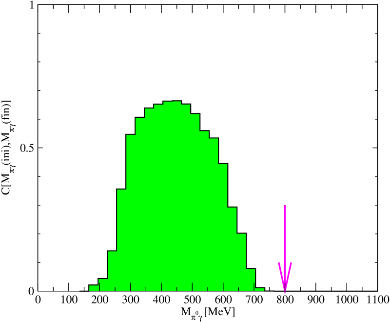
Figure 5: The correlation function $C(M_{\pi\gamma}(ini),M_{\pi\gamma}(fin))$ (see the details in the text)

Acknowledgments

We would like to thank V. Metag, M. Nanova, S. Friedrich and M. Kotulla for discussions on the issue and on the experimental data. Useful information on mixed events was provided by C. Djalali and R. Nasseripour. This work was supported by DFG through the SFB/TR16, by DGI and FEDER funds, under contracts FIS2006-03438, FPA2007-65748, The Generalitat Valenciana in the Prometeo Program and the Spanish Consolider-Ingenio 2010 Programme CPAN (CSD2007-00042), by Junta de Castilla y León under contract SA 016A07 and GR12, and it is part of the EU integrated infrastructure initiative Hadron Physics Project under contract number RII3-CT-2004-506078.

References

- (1) V. Bernard and U. G. Meissner, Nucl. Phys. A 489, 647 (1988).
- (2) G. E. Brown and M. Rho, Phys. Rev. Lett. 66, 2720 (1991).
- (3) R. Rapp, G. Chanfray and J. Wambach, Nucl. Phys. A 617, 472 (1997) [arXiv:hep-ph/9702210].
- (4) M. Urban, M. Buballa and J. Wambach, Nucl. Phys. A 673, 357 (2000) [arXiv:nucl-th/9910004].
- (5) D. Cabrera, E. Oset and M. J. Vicente Vacas, Nucl. Phys. A 705, 90 (2002) [arXiv:nucl-th/0011037].
- (6) R. Arnaldi et al. [NA60 Collaboration], Phys. Rev. Lett. 96, 162302 (2006) [arXiv:nucl-ex/0605007].
- (7) S. Damjanovic et al. [NA60 Collaboration], Nucl. Phys. A 783, 327 (2007) [arXiv:nucl-ex/0701015].
- (8) M. H. Wood et al. [CLAS Collaboration], arXiv:0803.0492 [nucl-ex].
- (9) R. Muto et al. [KEK-PS-E325 Collaboration], Phys. Rev. Lett. 98, 042501 (2007) [arXiv:nucl-ex/0511019].
- (10) M. Naruki et al., Phys. Rev. Lett. 96, 092301 (2006) [arXiv:nucl-ex/0504016].
- (11) P. Muhlich, T. Falter and U. Mosel, Eur. Phys. J. A 20, 499 (2004) [arXiv:nucl-th/0310067].
- (12) M. Kaskulov, E. Hernandez and E. Oset, Eur. Phys. J. A 31, 245 (2007) [arXiv:nucl-th/0610067].
- (13) M. Kaskulov, H. Nagahiro, S. Hirenzaki and E. Oset, Phys. Rev. C 75, 064616 (2007) [arXiv:nucl-th/0610085].
- (14) David Trnka Thesis, University of Giessen.
- (15) D. Trnka et al. [CBELSA/TAPS Collaboration], Phys. Rev. Lett. 94, 192303 (2005) [arXiv:nucl-ex/0504010].
- (16) M. Kotulla et al. [CBELSA/TAPS Collaboration], Phys. Rev. Lett. 100, 192302 (2008) [arXiv:0802.0989 [nucl-ex]].
- (17) V. Metag, Prog. Part. Nucl. Phys. 61, 245 (2008) [arXiv:0711.4709 [nucl-ex]].
- (18) Mariana Nanova, Talk given at the XIII International Conference on Hadron Spectroscopy, December 2009, Florida State University.
- (19) M. Kotulla, private communication.
- (20) A. Braghieri et al., Phys. Lett. B 363, 46 (1995).
- (21) F. Harter et al., Phys. Lett. B 401, 229 (1997).
- (22) M. Wolf et al., Eur. Phys. J. A 9, 5 (2000).
- (23) S. Schadmand, Pramana 66, 877 (2006) [arXiv:nucl-ex/0505023].
- (24) U. Thoma, Phys. Lett. B 659, 87 (2008) [arXiv:0707.3592 [hep-ph]].
- (25) U. Thoma, Int. J. Mod. Phys. A 20, 280 (2005).
- (26) J. Ajaka et al., Phys. Lett. B 651, 108 (2007).
- (27) M. Ripani et al., Phys. Atom. Nucl. 63, 1943 (2000) [Yad. Fiz. 63, 2036 (2000)].
- (28) M. Ripani et al. [CLAS Collaboration], Phys. Rev. Lett. 91, 022002 (2003) [arXiv:hep-ex/0210054].
- (29) V. D. Burkert et al., Phys. Atom. Nucl. 70, 427 (2007) [Yad. Fiz. 70, 457 (2007)].
- (30) J. A. Gomez Tejedor and E. Oset, Nucl. Phys. A 600, 413 (1996) [arXiv:hep-ph/9506209].
- (31) V. Bernard, N. Kaiser and U. G. Meissner, Phys. Lett. B 382, 19 (1996) [arXiv:nucl-th/9604010].
- (32) J. C. Nacher, E. Oset, M. J. Vicente and L. Roca, Nucl. Phys. A 695, 295 (2001) [arXiv:nucl-th/0012065].
- (33) J. C. Nacher and E. Oset, Nucl. Phys. A 697, 372 (2002) [arXiv:nucl-th/0106005].
- (34) K. Ochi, M. Hirata and T. Takaki, Phys. Rev. C 56, 1472 (1997) [arXiv:nucl-th/9703058].
- (35) W. Roberts and T. Oed, Phys. Rev. C 71, 055201 (2005) [arXiv:nucl-th/0410012].
- (36) M. Nanova for the CBELSA/TAPS Collaboration, Proceedings of the Workshop on the Physics of Excited Nucleons NSTAR 2005, Florida State University, Tallahassee, 12-15 October 2005, edited by S. Capstick et al. (World Scientific, Singapore, 2006) p. 359.
- (37) T. Nakabayashi et al., Phys. Rev. C 74, 035202 (2006).
- (38) J. Ajaka et al., Phys. Rev. Lett. 100, 052003 (2008).
- (39) I. Horn et al. [CB-ELSA Collaboration], Eur. Phys. J. A 38, 173 (2008) [arXiv:0806.4251 [nucl-ex]].
- (40) M. Doring, E. Oset and D. Strottman, Phys. Rev. C 73, 045209 (2006) [arXiv:nucl-th/0510015].
- (41) M. Doring, E. Oset and D. Strottman, Phys. Lett. B 639, 59 (2006) [arXiv:nucl-th/0602055].
- (42) D. Drijard, H. G. Fischer and T. Nakada, Nucl. Instrum. Meth. A 225, 367 (1984).
- (43) P. Fachini [STAR Collaboration], J. Phys. G 28, 1599 (2002) [arXiv:nucl-ex/0203019].
- (44) D. L’Hote, Nucl. Instrum. Meth. A 337, 544 (1994).
- (45) N. van Eijndhoven and W. Wetzels, Nucl. Instrum. Meth. A 482, 513 (2002) [arXiv:hep-ph/0101084].
- (46) A. Toia [PHENIX Collaboration], Nucl. Phys. A 774, 743 (2006) [arXiv:nucl-ex/0510006].