Identical two-particle interferometry in diffraction gratings

Abstract

We study diffraction and interference of indistinguishable particles. We consider some examples where the wavefunctions and detection probabilities can be evaluated in an analytical way. The diffraction pattern of a two-particle system shows notorious differences for the cases of bosons, fermions and distinguishable particles. In the example of near-field interferometry, the exchange effects for two-fermion systems lead to the existence of planes at which the probability of double detection is null. We also discuss the relation with the approach to systems of identical particles based on correlation functions. In particular, we shall see that these functions reflect, as in noise interferometry, the underlying periodic structure of the diffraction grating.

1 Introduction

Exchange effects, associated with the peculiar behaviour of indistinguishable particles, have been extensively studied in the literature. In recent times these studies have followed two principal lines. On the one hand, the experimental measurement of correlation functions has corroborated the existence of bunching and antibunching effects. On the other hand, some interference phenomena are strongly dependent on the distinguishable or undistinguishable nature of the particles involved. In this paper we shall be mainly concerned with this second line of research.

In the case of photons, following the seminal work of Hong-Ou-Mandel (HOM)[1], the effects of the statistics of the particles have been extensively studied for interferences originated by the interaction in a beam splitter. Some authors have considered the extension of that approach to the case of massive particles. In [2] (and references therein) the behaviour of fermions in Mach-Zehnder interferometers has been analyzed. The proposal presented in [3, 4], is also interesting, where an electronic HOM-type interferometer is used to detect entanglement. In all the above arrangements the particles can only be detected in the output arms of a beam splitter or interferometer. We analyse in this paper whether exchange effects are also present in other interferometric arrangements with a continuous spatial distribution. The natural framework to discuss this possibility is that of diffraction gratings, which generate continuous spatial patterns.

At this point we must signal the existence of other works by Mandel’s group where the spatial dependence of two-photon interferences has been analysed [5, 6]: two photons generated by down-conversion interfere at a beam splitter and detectors are placed in the two output arms. Moving the detectors relative to

the beam splitter, a spatial two-photon interference pattern is observed. At variance with our goal, these interferences are generated at a beam splitter and not at a diffraction grating.

As a first approximation to the problem, we consider in this paper some simple examples of diffraction and interference by gratings which can be solved analytically. This way we can illustrate the main ideas involved in the problem without addressing other more technical questions. To be concrete, we shall analyse two archetypical systems:

(i) Diffraction by a single slit of a Gaussian wave packet. This is probably the simplest system where the effects can be analysed. We shall evaluate the probability detection patterns showing sharp differences between two-particle distributions of bosons, fermions and distinguishable particles.

(ii) Near-field interferometry with periodic gratings. The best known example of this type of arrangement is the Talbot Lau interferometer [7, 8], which has been used in a number of interesting studies in matter wave interferometry [8, 9]. In this case we shall find a novel characteristic associated with the statistics of the system. For a pair of indistinguishable fermions, there are planes with a null probability of double detection.

As signaled before, in the other principal line of study of indistinguishable systems the focus is on the correlation functions. This line originated in the seminal work of Hanbury Brown and Twiss (HBT) [10], in which they counted joint detections (in two separate detectors) of photons from different chaotic sources. The correlations showed that the photons tend to arrive bunched in groups. This behavior can be understood within a classical framework if one introduces fluctuating phases. In contrast, the opposite trend observed for fermions has no classical analogue. Then the only framework able to completely describe bunching and antibunching is the quantum one, where these effects can be explained in an unified way in terms of constructive and destructive interference. In the last years, the correlation functions of free boson [11, 12, 13] and fermions [14, 15, 13] have been experimentally obtained, corroborating the existence of bunching and antibunching effects. It is natural to ask for the behaviour of the correlation functions in interferometry and to see if the presence of interference effects can modify the usual picture. A well-suited technique for the position-sensitive counting of particles when one is concerned with the spatial dependence of the correlations is noise interferometry. This technique converts spatial patterns into an interference signal. In particular, in Refs. [12, 15] the existence of periodic quantum correlations was shown between density fluctuations in an expanding atom cloud when released from an optical trap. These spatial correlations reflect the underlying ordering in the lattice trap. Noise interferometry, is useful for identifying quantum phases of ultracold atoms in periodic potentials. We shall evaluate the correlation functions in the framework (ii) showing that, as in noise interferometry, they reflect the periodic structure of the underlying arrangement.

The plan of the paper is as follows. In Sect. 2 we present the basic equations and derive some general properties of the interference of two identical particles in a diffraction grating. The two analytically solvable models considered in the paper are discussed in Sects. 3 (diffraction) and 4 (near-field interferometry). The last one is divided into two subsetions devoted, respectively, to single- and multi-mode states. Section 5 deals with the behaviour of correlation functions in diffraction gratings. Finally, in Sect. 6, we recapitulate on the principal results of the paper and consider the possibility of testing them.

2 General expressions

The arrangement we consider here consists in a system of two identical particles arriving on a diffraction grating. After the diffraction grating we place detectors measuring the interference pattern, which is obtained after many repetitions of the experiment.

We denote by $\psi_{\bf k}({\bf x},t)$ and $\psi_{\bf p}({\bf y},t)$ the wavefunctions of the two particles, where ${\bf x}$ and ${\bf y}$ are the coordinates of the particles and ${\bf k}$ and ${\bf p}$ are their wavevectors or momenta. When the particles are in single-mode states, they refer to the wavevectors or momenta of these modes. On the other hand, if we are dealing with multi-mode distributions, they represent the mean values of these distributions. When the particles are identical the usual product wavefunction $\psi_{\bf k}({\bf x},t)\psi_{\bf p}({\bf y},t)$, must be replaced by

$$\frac{1}{\sqrt{2}}\left(\psi_{\bf k}({\bf x},t)\psi_{\bf p}({\bf y},t)\pm\psi_{\bf p}({\bf x},t)\psi_{\bf k}({\bf y},t)\right)$$ (1)

In the double sign expressions the upper one holds for bosons and the lower one for fermions. The probabilities associated with this wavefuntion are

$$P({\bf x},{\bf y},t)=\frac{1}{2}|\psi_{\bf k}({\bf x},t)|^{2}|\psi_{\bf p}({\bf y},t)|^{2}+\frac{1}{2}|\psi_{\bf p}({\bf x},t)|^{2}|\psi_{\bf k}({\bf y},t)|^{2}$$

$$\pm Re(\psi_{\bf p}^{*}({\bf y},t)\psi_{\bf k}^{*}({\bf x},t)\psi_{\bf k}({\bf y},t)\psi_{\bf p}({\bf x},t))$$ (2)

We have an interference term that is not present for distinguishable particles, according to the standard interpretation of exchange effects as interference effects. From now on, in order to avoid any possible confusion by the use of the interference concept in two different ways, we restrict it to the effects induced by diffraction gratings. The interference effects associated with the indistinguishable character of the particles will be denoted as exchange effects.

It must be remarked that the (anti)symmetrization procedure is only physically required when there is a non-negligible overlapping between the two wavefunctions. If not, the particles must be treated as distinguishable ones. The important point is that once the overlapping has taken place, due to the linearity of the evolution equations, the (anti)symmetric form of the two-particle wavefunction persists at subsequent times.

Several consequences directly emerge from the above expressions:

(a) For bosons in the same state (${\bf p}={\bf k}$), the probability of simultaneous detection of two bosons at the same point is $P({\bf x},{\bf x},t)=2|\psi_{\bf p}({\bf x},t)|^{4}$. The probability is proportional to the fourth power of the wavefunction modulus. This behaviour was described in models of double ionization by massive particles [16] and double absorption of massive particles [17]. At this point a word of caution is in order if one tries to experimentally corroborate the above probability distribution. The probability in Eq. (2) for different points, ${\bf x}\neq{\bf y}$, can be experimentally measured using two detectors placed at ${\bf x}$ and ${\bf y}$. In the case of double (boson) detection at the same point ${\bf x}={\bf y}$, we can only use one detector, which must be able to distinguish between single- and double-detection events. This type of detector is already available for photons [18, 19], but up to our knowledge, not for massive particles.

(b) For fermions the wavefunction of the complete system can have nodal points not present for factorizable ones. For example, if the individual wavefunctions obey (up to a global phase) the relations $\psi_{\bf k}({\bf X},t)=\psi_{\bf p}({\bf X},t)$ for a pair of points ${\bf X}$ and ${\bf Y}$, these points are nodal ones of the two-particle wavefunction (not present in the factorizable case $\psi_{\bf k}({\bf X},t)\psi_{\bf p}({\bf Y},t)$ unless ${\bf X}$ or ${\bf Y}$ are themselves nodal points). This property will play a central role in the discussion of the detection distributions in near-field arrangements.

(c) The set of points $({\bf X},{\bf Y},t)$ has another interesting property (for bosons and fermions). The detection probabilities at these points show a maximal deviation with respect to distinguishable ones. A good measure to quantify how much the detection rate is enhanced or diminished by the presence of the exchange effects is given by the ratio of the detection rates for idistinguishable particles and for the same state without exchange effects. It is defined at each point and at a given time as

$${\cal R}({\bf x},{\bf y},t)=\frac{P({\bf x},{\bf y},t)}{P_{NE}({\bf x},{\bf y},t)}$$ (3)

where $P_{NE}$ denotes the probability distribution without interchange effects. In the particular case of the set $({\bf X},{\bf Y},t)$ we obtain the maximum difference,

$${\cal R}({\bf X},{\bf Y},t)=\frac{(1\pm 1)|\psi_{\bf k}({\bf X},t)|^{2}|\psi_{\bf k}({\bf Y},t)|^{2}}{|\psi_{\bf k}({\bf X},t)|^{2}|\psi_{\bf k}({\bf Y},t)|^{2}}=1\pm 1$$ (4)

which is $2$ for bosons and $0$ for fermions. The rate of simultaneous detections for bosons doubles that without exchange effects, whereas that of fermions drops to zero. The resemblances with the bunching and antibunching effects are clear, although in this case the points ${\bf X}$ and ${\bf Y}$ (at a given time $t$) do not need to be very close. The particles were close enough only at a previous time, leading to the (anti)symmetrization of the wavefunction, which persists at subsequent times.

In order to go beyond these general properties and to look for other effects, we must consider particular arrangements and evaluate the form of the wavefunctions in each situation. We do it in the next two sections.

3 Diffraction

We consider in this section the diffraction of a pair of indistinguishable particles by a slit. The rigorous analysis of the problem leads to the numerical integration of Fresnel s functions [20, 21]. A simpler approach to the problem is, following Feynman [20], to replace the slit by a Gaussian slit. With this approximation we have an analytically solvable problem. The wave packet generated by this slit with soft edges has also a Gaussian profile in the direction parallel to the slit. The movement in the perpendicular direction is assumed to be unaffected. As usual in the treatment of the problem, we consider a two-dimensional problem, neglecting the vertical axis. Moreover, as the movement in the perpendicular axis is almost unaffected, the relevant physics is contained in the parallel axis and the problem reduces to an one-dimensional one.

The simplest way to study multimode states is to assume that the wavevector distribution of each particle is a Gaussian one [21]. Using the notation of Ref. [21] the one-dimensional Gaussian distribution is $f(k)=(4\pi)^{1/4}\sigma^{-1/2}\exp(-(k-k_{0})^{2}/2\sigma^{2})$ with $\sigma$ the width of the distribution and $k_{0}$ its central value. The wavefunction is obtained by superposing a set of planes waves with that distribution ($(2\pi)^{-1}\int dkf(k)\exp(i(kx-E_{k}t/\hbar))$ with $E_{k}=\hbar^{2}k^{2}/2m$)[21]:

$$\psi(x,t)=C(t)\exp\left(\frac{-\sigma^{2}(x-vt)^{2}+ik_{0}(2x-vt)+i\hbar\sigma^{4}x^{2}t/m}{\mu(t)}\right)$$ (5)

with $v=\hbar k_{0}/m$,

$$C(t)=\pi^{-1/4}\left(\frac{1}{\sigma}+\frac{i\hbar\sigma t}{m}\right)^{-1/2}$$ (6)

and

$$\mu(t)=2\left(1+\frac{\hbar^{2}\sigma^{4}t^{2}}{m^{2}}\right)$$ (7)

Note the absence with respect to the formula in [21] of a multiplicative coefficient $2$ in the last term of the numerator in the exponential.

As required by our assumption of a Gaussian slit, the wavefunction has the form (up to some phase terms) of a spatial Gaussian packet with time-dependent width $\sigma^{-2}+(\hbar^{2}t^{2}\sigma^{2}/m^{2})$.

Using the expression of the wavefunction, it is immediate to evaluate the probability distribution for two indistinguishable particles. We assume both particles to be in states of the type (5), with the same width and central wavevectors $k_{0}$ and $p_{0}$. The final result is

$$P(x,y,t)/|C(t)|^{4}=\frac{1}{2}\left(e^{A}+e^{B}\pm 2e^{(A+B)/2}\cos\left(\frac{2}{\mu(t)}(x-y)(k_{0}-p_{0})\right)\right)$$ (8)

with

$$A=-\frac{2\sigma^{2}}{\mu(t)}((x-v_{k}t)^{2}+(y-v_{p}t)^{2})$$ (9)

and $B$ given by a similar expression with the interchange of $v_{k}$ and $v_{p}$.

From the above expressions it is clear that the detection probabilities for a pair of indistinguishable particles show notorious differences with respect to those of distinguishable ones. We illustrate this point numerically in Fig. 1, where we compare the probability of simultaneous detection for bosons, fermions and distinguishable particles. In order to simplify the presentation, we fix one of the points, $x=x_{0}$, and evaluate the detection probability for arbitrary $y$. We choose for $x_{0}$, at a fixed time $t$, the value $x_{0}=v_{k}t$ which maximizes the detection probability in the first exponential. The probability in the case of distinguishable particles is $P_{dis}(x,y,t)/|C(t)|^{4}=e^{A}(x=x_{0})=\exp(-2\sigma^{2}(y-v_{p}t)^{2}/\mu(t))$. Taking $\hbar t/m=0.1$, $k_{0}=1=-p_{0}$ and a width of the distribution $\sigma^{2}=0.125$ we have the following distribution:

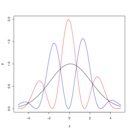
Figure 1: In the vertical axis we represent, in arbitrary units, $p=P(x_{0},y,t)/|C(t)|^{4}$. In the horizontal axis we have the coordinate $y$, also in arbitrary units, and the point $0$ corresponding to $y=v_{p}t$. The red, black and blue curves correspond, respectively, to bosons, distinguishable particles and fermions.

Several consequences emerge directly from the figure. As expected, the distribution in the distinguishable case retains a Gaussian form centred around the point $y=v_{p}t$. In contrast, for both fermions and bosons, the mathematical form of the curves departs from the Gaussian profile showing the typical form of an interference pattern. The maximum probability for bosons is approximately at the same position of the peak of the Gaussian for distinguishable particles and doubles its value. At the same position we have a null-probability point for fermions.

All the above development has been done in terms of the diffraction by a slit. However, these expressions also describe two particles that interact (there must be a strong overlapping between them) at a given moment and then continue a free evolution. We can measure the positions of the particles after the interaction, which are given by Eq. (8). Note that in this case that expression is exact, whereas for the description of the diffraction by the slit, it is only an approximation.

4 Near-field interferometry

After considering an example of diffraction, we now move to a purely interferometric arrangement, which illustrates other types of effects associated with the interchange terms. In particular, we focus on near-field interference in the eikonal approximation [8], which can be tackled analytically (for the limitations of the eikonal approximation see [22]). One of the best known examples of near-field arrangement is the Talbot Lau one [7], which has important applications in matter wave interferometry [8, 9]. In order to emphasize on the main physical ideas of the problem without excessive mathematical technicalities, in a first step we shall only consider particles in single-mode states, showing later that the main result persists (under adequate restrictions) in the more realistic framework of multi-mode states.

4.1 Single-mode states

We consider a plane wave $\psi_{o}=\exp(ikz)$ which incides on a grating placed in the plane perpendicular to the z-axis. If the grating function is a periodic one, the transmission function is given by

$${\cal T}(x)=\sum_{n}A_{n}\exp(2\pi inx/d)$$ (10)

with $n$ an integer, $d$ the grating period and $A_{n}=|A_{n}|\exp(i\xi_{n})$ the coefficient of the term $n$. The wavefunction at a distance $L$ behind the grating is [8]:

$$\psi_{k}^{L}(x)=e^{ikL}\sum_{n}A_{n}\exp\left(\frac{2\pi inx}{d}\right)\exp\left(-\frac{i\pi n^{2}L\lambda_{k}}{d^{2}}\right)$$ (11)

with $\lambda_{k}$ the wavelength of the particle and $x$ the coordinate of the axis in which we measure the interferences.

We consider now the normalization of this wavefunction. From the expression

$$|\psi_{k}^{L}(x)|^{2}=\sum_{n,m}A_{n}^{*}A_{m}\exp\left(\frac{2\pi i(m-n)x}{d}\right)\exp\left(-\frac{i\pi L(m^{2}-n^{2})\lambda_{k}}{d^{2}}\right)$$ (12)

we see that $\int_{-\infty}^{\infty}|\psi_{k}^{L}(x)|^{2}dx$ is not bound. In effect, the integration of the constant terms $A_{0}^{*}A_{0},A_{1}^{*}A_{1},\cdots$ does not give a finite value. One possibility to overcome this difficulty is to do the normalization in a relative sense, ${\cal N}^{-1}\int_{-\infty}^{\infty}|\psi_{k}^{L}(x)|^{2}dx=1$, with ${\cal N}=(\sum_{n}|A_{n}|^{2})\int_{-\infty}^{\infty}dx$. An alternative form of normalization is to consider the integration over the period $d$, $\frac{1}{d}\int_{0}^{d}dx|\psi_{k}^{L}(x)|^{2}=1$. Taking into account that $\int_{0}^{d}dx\exp(2\pi inx/d)=d\delta_{n0}$, we have $\frac{1}{d}\int_{0}^{d}dx|\psi_{k}^{L}(x)|^{2}=\sum_{n}|A_{n}|^{2}=A^{2}$, and the normalization condition is obtained dividing by $A$. It is simple to see that the same condition is reached using the relative normalization condition. The normalized wavefunction after the diffraction arrangement is given by $\psi_{k}^{L}(x)/A$, or equivalently by Eq. (11) with the replacement $A_{i}\rightarrow a_{i}=A_{i}/A$ ($a_{i}=|A_{i}/A|exp(i\xi_{n})$).

As anticipated in Sect. 2 let us consider the points $X$ where the condition $\psi_{k}^{L}(X)=\psi_{p}^{L}(X)$ holds (up to a global phase). In this example, the problem is stationary and we do not need to include explicitly the time variable. We introduce the new parameter

$$\phi_{kp}=\frac{\pi L}{d^{2}}(\lambda_{k}-\lambda_{p})$$ (13)

For all the initial wavevectors fulfilling the condition $\phi_{kp}=2\pi n_{*}$, with $n_{*}$ an integer, we have that at all the points $X$ contained in the plane defined by $z=L$, the wavefunctions obey the relation

$$\psi_{k}^{L}(X)=e^{i(k-p)L}\psi_{p}^{L}(X)$$ (14)

From now on, we restrict our considerations to fermions. The antisymmetrized wavefunction at that plane becomes null:

$$\frac{1}{\sqrt{2}}(\psi_{k}^{L}(X)\psi_{p}^{L}(Y)-\psi_{p}^{L}(X)\psi_{k}^{L}(Y))\rightarrow$$

$$\frac{1}{\sqrt{2}}e^{i(k-p)L}(\psi_{p}^{L}(X)\psi_{p}^{L}(Y)-\psi_{p}^{L}(X)\psi_{p}^{L}(Y))=0$$ (15)

For all the initial wavevectors for which the relation $\phi_{kp}=2\pi n_{*}$ holds, we have that in the plane $z=L$, there cannot be two-fermion detections. Conversely, once the values of $\lambda_{k}$ and $\lambda_{p}$ are fixed, there are always planes in which the phenomenon can be observed. These planes are given by $z=L_{n}$, with $L_{n}=2nd^{2}/(\lambda_{k}-\lambda_{p})$ and $n$ any integer. All the points in these planes are nodal points of the two-fermion wavefunction.

Note that this result does not forbid one-fermion detections at these planes. In effect, the one-fermion detection probabilities are given by the reduced detection probabilities, ${\cal P}(X)=\int P(X,y)dy$. The integration on $y$ contains any $y$ placed on any plane, not only the $Y^{\prime}s$ contained in the nodal plains. The contributions of the points in the nodal plains are null, $P(X,Y)=0$, but the contributions $P(X,y)$ with $y$ outside these special planes can be different from zero. The sum of all these contributions can be, in principle, different from zero leading to a non-null one-fermion distribution at the nodal planes.

4.2 Multi-mode states

We move now to the more realistic case of non-monochromatic states. We show that the result of the previous subsection is still valid for narrow enough initial wavepackets.

If the momentum distribution of the wavepacket is $f(k)$, the wavefunction at a distance $L$ behind the grating becomes

$$\psi_{f}^{L}(x)=\sum_{n}A_{n}F_{n}\exp\left(\frac{2\pi inx}{d}\right)$$ (16)

with

$$F_{n}=\int dkf(k)e^{ikL}e^{(-i\pi n^{2}L\lambda_{k}/d^{2})}\sim$$

$$e^{ik_{0}L}e^{(-i\pi n^{2}L\lambda_{k_{0}}/d^{2})}\int dke^{-(k-k_{0})^{2}/2\sigma^{2}}e^{i(k-k_{0})L}e^{(-i\pi n^{2}L(k_{0}-k)/d^{2}kk_{0})}$$ (17)

where we have adopted for the mode distribution a Gaussian curve with the central wavevector $k_{0}$. In order to simplify the notation, we have dropped the coefficients associated with its normalization.

The two imaginary exponentials inside the integral have a joint argument $L(k-k_{0})(1+(\pi n^{2}/d^{2}kk_{0}))$. When the condition $d^{2}kk_{0}\gg\pi n^{2}$ holds, the integral simplifies to $I(k_{0})=\int dke^{-(k-k_{0})^{2}/2\sigma^{2}}e^{i(k-k_{0})L}$. Let us consider the circumstances under which this approximation can be justified. Three conditions must be fulfilled. (1) $n$ must be small. For large values of $n$ the right-hand side of the inequality will be very large and the term containing it cannot be neglected. Thus, the summation in (16) must be truncated at some value $n_{0}$. This truncation is plainly justified because most of the behaviour of the system can be described taking into account only the lower terms in the summation. As a matter of fact, in the representative experiment in [8] the interference signal is essentially determined by the $0$ and $\pm 1$ components only. (2) For values of $k$ close to the central one, $k_{0}$, we must have $d^{2}kk_{0}\approx d^{2}k_{0}^{2}\gg\pi n_{0}^{2}$. This condition can be fulfilled by restricting our considerations to this range of central wavevectors. (3) As a consequence of (2), the distribution must be sharp enough around $k_{0}$ in order the contribution of the elements with $|k|\ll|k_{0}|$ to be negligible.

With this approximation Eq. (16) becomes:

$$\psi_{k_{0}}^{L}(x)=\sum_{|n|\leq|n_{0}|}A_{n}I(k_{0})e^{ik_{0}L}e^{(-i\pi n^{2}L\lambda_{k_{0}}/d^{2})}e^{(2\pi inx/d)}$$ (18)

Let us consider now another distribution with the same Gaussian form (the same width), but centered around another value $p_{0}$. Then $I(k_{0})=I(p_{0})$, and we are at the same position of the previous subsection: when the relation $\phi_{k_{0}p_{0}}=2\pi n_{*}$ holds we have that in the plane $z=L$ the wavefunctions obey $\psi_{k_{0}}^{L}(X)=e^{i(k_{0}-p_{0})L}\psi_{p_{0}}^{L}(X)$.

Within the range of validity of this approximation, the result obtained in the previous subsection for a single-mode initial wavefunction can be extended to its multi-mode counterpart.

5 Correlation functions

As signaled in the introduction, another fundamental line of research in identical particles is based on correlation functions. We analyse in this section whether the presence of the interference device modifies the behaviour of the functions found in free systems or optical lattices.

The correlation function is defined as

$$C(\eta)=\frac{1}{d}\int_{0}^{d}P(x,x+\eta)dx$$ (19)

To calculate this expression we must evaluate the two-particle probability distribution. In order to simplify the calculations, we restrict our considerations to the case of particles described by single-mode plane waves. As we have seen in the previous section, the result obtained for a mono-chromatic particle can be extended to sharp enough wave packets. We analyse the correlations in a fixed plane $z=L$. The two detectors measuring the correlations must be placed in that plane. Then it is not necessary to include the $L$ parameter explicitly as a superscript of the wavefunction.

The modulus of the initial state is:

$$|\psi_{k}(x)|^{2}=1+2\sum_{n,m}^{m>n}|a_{n}a_{m}|\cos\left(\frac{2\pi(m-n)x}{d}-\frac{\pi L(m^{2}-n^{2})\lambda_{k}}{d^{2}}+\xi_{m}-\xi_{n}\right)$$ (20)

In order to complete the expression for the probability, we must evaluate the crossed or interference term

$$Re(\psi_{p}^{*}(y)\psi_{k}^{*}(x)\psi_{k}(y)\psi_{p}(x))=Re\sum_{n,m,r,s}a_{n}^{*}a_{m}^{*}a_{r}a_{s}\times$$

$$\exp\left(\frac{2\pi i[(s-n)x+(r-m)y]}{d}\right)\exp\left(-\frac{i\pi L[\lambda_{p}(s^{2}-m^{2})+\lambda_{k}(r^{2}-n^{2})]}{d^{2}}\right)=$$

$$\sum_{n,m,r,s}|a_{n}a_{m}a_{r}a_{s}|\times$$ (21)

$$\cos\left(\frac{2\pi[(s-n)x+(r-m)y]}{d}-\frac{\pi L[\lambda_{p}(s^{2}-m^{2})+\lambda_{k}(r^{2}-n^{2})]}{d^{2}}+\xi_{r,s,n,m}\right)$$

where $\xi_{r,s,n,m}=\xi_{r}+\xi_{s}-\xi_{n}-\xi_{m}$. Adding the direct and crossed terms, we obtain for the probability

$$P({\bf x},{\bf y})=1+$$

$$\sum_{m,n}^{m>n}|a_{n}a_{m}|(\cos\varphi_{m,n}^{k}({\bf x})+\cos\varphi_{m,n}^{p}({\bf x})+\cos\varphi_{m,n}^{k}({\bf y})+\cos\varphi_{m,n}^{p}({\bf y}))+$$

$$2\sum_{n,m,r,s}^{m>n,r>s}|a_{n}a_{m}a_{r}a_{s}|(\cos\varphi_{m,n}^{k}({\bf x})\cos\varphi_{r,s}^{p}({\bf y})+\cos\varphi_{m,n}^{p}({\bf x})\cos\varphi_{r,s}^{k}({\bf y}))\pm$$

$$\sum_{n,m,r,s}|a_{n}a_{m}a_{r}a_{s}|\times$$ (22)

$$\cos\left(\frac{2\pi[(s-n)x+(r-m)y]}{d}-\frac{\pi L[\lambda_{p}(s^{2}-m^{2})+\lambda_{k}(r^{2}-n^{2})]}{d^{2}}+\xi_{r,s,n,m}\right)$$

where $\varphi_{m,n}^{k}(x)=\frac{2\pi(m-n)x}{d}-\frac{\pi L(m^{2}-n^{2})\lambda_{k}}{d^{2}}+\xi_{m}-\xi_{n}$. Now, the correlation function can be obtained from Eq. (22). The calculation is simple but lengthy. There are four types of contributions: (i) constant terms, (ii) terms containing $\cos\varphi_{m,n}^{k}(x)$, (iii) terms with $\cos\varphi_{m,n}^{k}(x)\cos\varphi_{s,r}^{p}(y)$ and (iv) those contained in the crossed term. Let us evaluate them separately.

(i) For constant terms we have, $\frac{1}{d}\int_{0}^{d}\;ctedx=cte$.

(ii) By direct calculation we have, $\frac{1}{d}\int_{0}^{d}\cos\varphi_{m,n}^{k}(x)dx=0=\frac{1}{d}\int_{0}^{d}\cos\varphi_{m,n}^{k}(x+\eta)dx$. The terms with this form do not contribute to the correlation function.

(iii) Using standard trigonometric relations and integrals we have that the integral $\frac{1}{d}\int_{0}^{d}\cos\varphi_{m,n}^{k}(x)\cos\varphi_{r,s}^{p}(x+\eta)dx$ equals $0$ when $m-n\neq\pm(r-s)$ and

$$\frac{1}{2}\cos\left(\frac{2\pi(s-r)\eta}{d}+\phi_{mnsr}^{kp}\right)+\frac{1}{2}\cos\left(\frac{2\pi(s-r)\eta}{d}+\phi_{mnsr}^{pk}\right)$$ (23)

otherwise, with $\phi_{mnsr}^{kp}=-\frac{\pi L}{d^{2}}[(m^{2}-n^{2})\lambda_{k}+(r^{2}-s^{2})\lambda_{p}]+\xi_{m}-\xi_{n}-\xi_{s}+\xi_{r}$.

(iv) For the crossed term, we must distinguish when $s-n+r-m$ is zero or different from zero. When it is not zero, we have again the situation (ii) and its contribution is null. On the other hand, when $s-n+r-m=0$, the integral of the cosine gives

$$\cos\left(\frac{2\pi(r-m)\eta}{d}+\Theta_{nmrs}^{kp}\right)$$ (24)

with $\Theta_{nmrs}^{kp}=-\frac{\pi L}{d^{2}}[(r^{2}-n^{2})\lambda_{k}+(s^{2}-m^{2})\lambda_{p}]+\xi_{r,s,n,m}$.

Combining all these expressions, we obtain the correlation function:

$$C(\eta)=1+2\sum_{n,m,r,s}^{m>n,s>r}|a_{m}a_{n}a_{s}a_{r}|\times$$

$$\left(\frac{1}{2}\cos\left(\frac{2\pi(s-r)\eta}{d}+\phi_{mnsr}^{kp}\right)+\frac{1}{2}\cos\left(\frac{2\pi(s-r)\eta}{d}+\phi_{mnsr}^{pk}\right)\right)\pm$$

$$\sum_{n,m,r,s}^{s-n+r-m=0}|a_{m}a_{n}a_{s}a_{r}|\cos\left(\frac{2\pi(r-m)\eta}{d}+\Theta_{nmrs}^{kp}\right)$$ (25)

The correlation function depends on the parameters of the grating, $a_{i}$ and $d$ and on the wavevectors of the incident particles (through $\phi_{mnsr}^{kp}$ and $\Theta_{nmrs}^{kp}$ both functions of $\lambda_{k}$ and $\lambda_{p}$). This behaviour is to be compared with that of free particles, for which the correlation function depends on the wavevectors in the form $C_{free}(\eta)=1\pm\cos((p-k)\eta)$ (for plane waves $\exp(ikx)$ and $\exp(ipy)$). The spatial periodicity of $C_{free}$ is determined by $p-k$. For interfering particles, however, the periodicity is only ruled by $d/n$ (with $n$ any integer), a function of the parameter of the grating $d$. In the correlation function we have all the periods ($d/n$) contained in the diffraction grating. The wavevectors only determine (in conjunction with $d$ and the coefficients $\xi_{i}$) a phase for each term. We conclude that, as in noise interferometry, the correlation functions reflect the underlying structure of the periodic grating.

A particularly clear illustration of the behaviour of the correlation functions is obtained in the particular case that only $a_{1}$ and $a_{0}$ are different from zero. Moreover, for the sake of simplicity, we assume the two coefficients to be real. The correlation function in this case is (using $a_{1}^{2}+a_{0}^{2}=1$)

$$C(\eta)=(1\pm 1)\pm 2a_{0}^{2}a_{1}^{2}(-1+\cos\phi_{kp})+2a_{0}^{2}a_{1}^{2}(\pm 1+\cos\phi_{kp})\cos\left(\frac{2\pi\eta}{d}\right)$$ (26)

Now there is only one periodicity, $d$. The wavevectors only determine (in conjunction with $a_{o}$ and $a_{1}$) the amplitude of the oscillations. Moreover, the dependence is in the form $\frac{1}{k}-\frac{1}{p}$, instead of $p-k$.

For short distances, $\eta\rightarrow 0$, we have $C_{F}(\eta)\sim\frac{C_{0}}{4}(\frac{2\pi}{d})^{2}\eta^{2}$ ($C_{0}=4a_{0}^{2}a_{1}^{2}(1-\cos\phi_{kp})$)and $C_{B}(\eta)-C_{B}(0)\sim-a_{0}^{2}a_{1}^{2}(\frac{2\pi}{d})^{2}(1+\cos\phi_{kp})\eta^{2}$ that is the usual dependence on $\eta^{2}$, but with different coefficients.

6 Discussion

In this paper we have analysed the behaviour of exchange effects in diffraction and interference. We have found the existence of some distinctive characteristics of this type of interferometry: modifications of the probability distributions with respect to those of distinguishable particles, strong increase or decrease of the double detection rates for some pairs of points (similar to bunching or antibunching, but without need of closeness between the particles) and existence of planes where the double detection of fermions is forbidden. On the other hand, the correlation functions show a behaviour similar to that found in noise interferometry, reflecting the periodic structure of the diffraction grating.

Now briefly address the question of how the above distinctive characteristics of continuous interferometry of identical particles can be tested experimentally. As signaled before, the interchange effects are present (and persist in the subsequent evolution of the system) when there is a non-negligible overlapping between the wavefunctions of the two particles at a given time. Then the key step is to obtain a non-negligible overlapping of the two particles at the time they reach the diffraction grating. This is equivalent to a careful preparation of the times of arrival of the two particles. In other words, the peaks of the two distributions must reach the grating at the same time. Because of recent progress in matter wave interferometry, interferometry of heavy molecules and the existence of massive systems with high degrees of coherence, these effects seem to be accessible to experimental scrutiny. Conversely, the presence of the effects described in this paper could be used as a test of the closeness of two particles under some specific preparation.

It must also be noted that because of the interaction of the beam with the grating, there can be absorption and backscatter processes which result in cases with zero or one particles arriving at the detectors. We can overcome this difficulty by considering a postselection process in which only events with two detections are taken into account.

In this paper we have restricted our considerations to two simple examples that can be treated analytically. Other types of diffraction gratings must be studied in order to see if (the same or different) exchange effects are also present.

Acknowledgments We acknowledge partial support from MEC (CGL 2007-60797).

References

- [1] Hong C K, Ou Z Y and Mandel L 1987 Phys. Rev. Lett. 59 2044
- [2] Silverman M P 1995 More Than One Mistery: Explorations in Quantum Interference (Springer Verlag, New York)
- [3] Giovannetti V 2006 Laser Phys. 16 1406
- [4] Giovannetti V et al. 2006 Phys. Rev. B 74 115315
- [5] Ghosh R, Hong C K, Ou Y and Mandel L 1986 Phys. Rev. A 34 3962
- [6] Ghosh R and Mandel L 1987 Phys. Rev. Lett. 59 1903. A modified and slightly improved version of the experiment was later described in Ou Z Y and Mandel L 1989 Phys. Rev. Lett 62 2941
- [7] Clauser J and Reinsch M 1992 App. Phys. B 54 380
- [8] Hackermüller L et al. 2003 App. Phys. B 77 781
- [9] Brezger B et al. 2002 Phys. Rev. Lett. 88 100404
- [10] Hanbury Brown R and Twiss R Q 1956 Nature 177 27
- [11] Yasuda M and Shimizu F 1996 Phys. Rev. Lett. 77 3090; Schellekens M et al. 2005 Science 310 648
- [12] Föllling S et al. 2005 Nature 434 481
- [13] Jeltes T et al. 2007 Nature 445 402
- [14] Henny M et al. 1999 Science 284 296; Oliver W D et al. 1999 Science 284 299; Kiesel H, Renz A and Hasselbach F 2002 Nature 418 392; Iannuzzi M et al. 2006 Phys. Rev. Lett. 96 080402
- [15] Rom T et al. 2006 Nature 444 733
- [16] Sancho P 2007 Phys. Lett. A 369 345
- [17] Sancho P 2008 Ann. Phys. 323 1271
- [18] Buzhan P et al. 2003 Nucl. Instr. Meth. Phys. Res. A 504 48
- [19] Eraerds P et al. 2007 Opt. Exp. 15 14539
- [20] Feynman R P and Hibbs A R 1965 Quantum Mechanics and Path integrals (McGraw-Hill)
- [21] Adams C S, Sigel M and Mlynek J 1994 Phys. Rep. 240 143
- [22] Nimmrichter S and Hornberger K 2008 Phys. Rev. A 78 023612