Multifrequency nature of the 0.75 mHz feature in the X-ray light curves of the nova V4743 Sgr

Abstract

We present timing analyses of eight X-ray light curves and one optical/UV light curve of the nova V4743 Sgr (2002) taken by Chandra and XMM-Newton on days after outburst: 50 (early hard emission phase), 180, 196, 302, 371, 526 (super soft source, SSS, phase), and 742 and 1286 (quiescent emission phase). We have studied the multifrequency nature and time evolution of the dominant peak at $\sim 0.75$ mHz using the standard Lomb-Scargle method and a 2-D sine fitting method. We found a double structure of the peak and its overtone for days 180 and 196. The two frequencies were closer together on day 196, suggesting that the difference between the two peaks is gradually decreasing. For the later observations, only a single frequency can be detected, which is likely due to the exposure times being shorter than the beat period between the two peaks, especially if they are moving closer together. The observations on days 742 and 1286 are long enough to detect two frequencies with the difference found for day 196, but we confidently find only a single frequency. We found significant changes in the oscillation frequency and amplitude. We have derived blackbody temperatures from the SSS spectra, and the evolution of changes in frequency and blackbody temperature suggests that the 0.75-mHz peak was modulated by pulsations. Later, after nuclear burning had ceased, the signal stabilised at a single frequency, although the X-ray frequency differs from the optical/UV frequency obtained consistently from the OM onboard XMM-Newton and from ground-based observations. We believe that the late frequency is the white dwarf rotation and that the ratio of spin/orbit period strongly supports that the system is an intermediate polar.

1 Introduction

Cataclysmic variables are interacting binary systems, consisting of a white dwarf primary and a late main sequence star, where accretion takes place from the cool companion to the white dwarf. If the accretion rate is in the range between $(1-4)\times 10^{-7}$ M_⊙ yr^-1, steady nuclear burning can establish, thus the hydrogen content of the accreted material is fused to helium at the accretion rate upon arrival on the white dwarf surface van den Heuvel et al. (1992). If the accretion rate is $<10^{-7}$ M_⊙ yr^-1 then the hydrogen-rich material settles on the white dwarf surface and ignites explosively in a thermonuclear runaway, after a critical amount of mass of $10^{-6}-10^{-4}$ M_⊙ (depending on white dwarf mass) has been reached. Such outbursts are commonly known as a Classical Nova outbursts. Within hours after outburst, the white dwarf is engulfed in an envelope of optically thick material that is driven away from the white dwarf by radiation pressure. Early in the evolution, the nova is bright in optical, but the peak of the spectral energy distribution shifts to higher energies as the mass ejection rate (and thus the opacity) decreases, exposing successively hotter layers (see, e.g., Bode & Evans 2008). A few weeks after outburst, the nova becomes bright in X-rays, and the observed X-ray spectra resemble those of the class of Super Soft Binary X-ray Sources (SSSs).

The nova V4743 Sgr was discovered in September 2002 by Haseda et al. (2002). The first measured envelope ejection velocities exceeded 1200 km s^-1 Kato et al. (2002). Nielbock & Schmidtobreick (2003) studied the nova at $\lambda$1.2 mm with the SEST instrument and concluded that the dominant emission source is the heated dust rather than free-free emission. The spectrum of the Nova was classified as Fe II type by Morgan et al. (2003). Petz et al. (2005) found significant absorption from Fe and N from atmosphere modelling to a SSS X-ray spectrum taken with Chandra 180 days after outburst, that had been presented earlier by Ness et al. (2003). Ness et al. found large-amplitude fast variability with a period of $\sim 22$ minutes with clear overtones of this signal in the periodogram. During this observation a strong decline in X-ray brightness was observed with simultaneous spectral change from continuum spectrum to emission lines. The count rate dropped from 44 counts per second to 0.6 within $\sim 6$ ks and stayed low for the rest of the observation (Ness 2010, in preparation). Kang et al. (2006) presented CCD unfiltered optical photometry analyses from observations taken in 2003 and 2005. They detected a period of 6.7 h which was interpreted as the orbital period of the underlying binary system. Six observations taken in short succession between days 1003 and 1011 days after outburst showed fast variability with a period of $\sim 24$ minutes. The authors attributed this signal to the beat period between the orbital and spin period of the white dwarf, where the 22 minute signal present in X-ray (Ness et al. 2003) was assumed to be the spin period of the central white dwarf. Sophisticated X-ray period studies were presented by Leibowitz et al. (2006). They reanalysed the Chandra data taken on day 180, together with an XMM-Newton observation taken on day 196. The large-amplitude variations were also found in the XMM-Newton data set. They detected at least 6 frequencies on day 180 and at least 12 on day 196. Most of the variability was explained by a combination of oscillations at a set of discrete frequencies, and the main feature with a period of $\sim 22$ minutes has a double peak in the periodogram. At least 5 signals were constant between the two observations. Leibowitz et al. (2006) suggested that the main feature in the periodogram at $\sim 22$ minutes ($\sim 0.75$ mHz) is related to the white dwarf spin and that the other observed frequencies are produced by non-radial white dwarf pulsations.

In this paper we present timing analyses of all Chandra and XMM-Newton observations, including those already analysed, for consistency. The main goal is to characterise the main feature at $\sim 0.75$ mHz and its possible multiple structure as well as following the evolution of the oscillations. We address the question whether these variations are produced by the white dwarf rotation or by its pulsations. In Sect. 2 we present all analysed X-ray data sets, and in Sect. 3 we describe our period analysis methods. The results are described in Sect. 4. This section is structured into the presentation of two different methods described in Sect. 3, the evolution of the oscillation amplitude of the main signal, studies on beat periods, and other signals within a larger frequency radius around the main signal as well as overtones. Our results are discussed in Sect. 5, and a summary with conclusions is given in Sect. 6.

2 Observations

In Table 1 we sumarise the analysed observations of the nova V4743 Sgr. The Chandra/ACIS (Nousek et al. 1987) light curve for day 50.2 was extracted from the level-two events file using a circular extraction region with radius 20 pixels. The Chandra/LETGS (Brinkman et al. 2000) light curves for days 180, 302, 371 and 526 were extracted from the non-dispersed photons (0th order), and the XMM-Newton/RGS light curve for day 196 was extracted from the dispersed photons. The two XMM-Newton/MOS (Turner et al. 2001) light curves for days 742 and 1286 were extracted from the events file using an extraction region with radius 200 pixels. In both observations, the source was on a chip gap in the pn, and only the MOS1 observations can be used.

In the XMM-Newton observation on day 742, additional optical/UV data from the Optical Monitor (OM, Talavera 2009) are available. Five light curves have been taken in series using the filters U, B, UVW1, UVM2, and UVW2 at 50-second time resolution. The different sensitivities of each filter are not of relevance to this paper, and the light curves shown in Fig. 2 are normalised. For the other XMM-Newton observations, the source was either too bright, or no timing mode was used.

Our focus is on the $\sim 0.75$ mHz period, and we thus removed all long-term variations by dividing the light curves by fifth-order polynomial fits. In Fig. 1 we show the de-trended, rebinned (100-s bins) light curves. For day 180, we only analyse the first 17 ks of data in order to avoid contamination by the steep decline that occurred shortly after (Ness et al. 2003). No such event occurred in any of the other observations, and the full data sets were used for all other observations.

For consistency checks, we have also extracted separate light curves for a hard and a soft band (15-30 Å and 30-40 Å, respectively), filtering on the wavelengths in the level 2 event files.

Table 1: Journal of observations. Given are ’Day’, days after outburst, ’Mission’, name of observing mission, ’$t$’, exposure time in seconds, ’$N$’, the number of time bins, ’$\Delta t$’, the duration of one time bin in seconds, and ’cr’, and mean count rate (counts per second). For day 180 we excluded the declining part of the light curve. In the text we refer to observations using days after outburst. For the optical/UV observation on day 742 we do not quote the mean count rate because of different filters used in the observation.

Day	Mission	$t$	$N$	$\Delta t$	cr
50.23	Chandra	5250	211	25	$0.2815\,\pm\,0.0001$
180.39	Chandra	17000	681	25	$35.2495\,\pm\,0.6472$
196.14	XMM/RGS	35280	1408	25	$52.0715\,\pm\,0.4411$
301.88	Chandra	11800	473	25	$35.0487\,\pm\,0.1449$
370.98	Chandra	12300	493	25	$17.7251\,\pm\,0.2687$
526.05	Chandra	10275	412	25	$3.7795\,\pm\,0.0345$
741.98	XMM/MOS1	22100	885	25	$0.0875\,\pm\,0.0016$
1285.9	XMM/MOS1	34050	682	50	$0.0579\,\pm\,0.0016$
741.98	XMM/OM	21722	206	100	–

Figure 1: Detrended and normalised X-ray light curves of all observations, indicated by the days after outburst given in the right legend of each panel (for observation log see Table 1). The detrending and normalisation was done using a 5-th order polynomial.

Figure 2: Optical/UV light curve taken in series with the XMM-Newton/OM on day 742 using different filters (upper panel) and corresponding Lomb-Scargle power spectrum with candidate frequency marked by dotted line (lower panel).

3 Period analysis techniques

The goal of this work is to study the dominant 0.75 mHz feature detected by Ness et al. (2003) and analysed in more detail by Leibowitz et al. (2006). The principal problem is the multifrequency nature of this dominant peak on day 196 (Leibowitz et al. 2006). While Ness et al. (2003) reported only one period in the power spectrum for day 180, Leibowitz et al. (2006) found two nearby frequencies, using a least square fitting approach. We note that the observation on day 180 is much shorter than that taken on day 196 (see Fig. 1 or Table 1), and a clear separation of multi-frequency oscillations is more difficult.

For our period analysis we use three different methods. First, we apply the standard Lomb-Scargle algorithm (Scargle 1982). This method calculates the normalised power for every frequency from the interval of interest with a selected frequency step. The result is a 2-D periodogram showing normalised power vs. tested frequency. The significant maxima are the significant signals.

We also use a linear combination of one or multiple sine curves that is fitted to the light curve. If $t_{i}$ defines a time grid, with $i$ indicating the index of each time bin, the model $s_{i}$ is defined on the same grid as

$$s_{i}=P_{i}+\overline{B_{i}}+\sum^{n}_{j=1}A_{j}{\rm sin}(2\pi t_{i}f_{j}+\phi_{j})\,,$$ (1)

where $P_{i}$ denotes a 5-th order polynomial used for detrending, $\overline{B_{i}}$ is the mean value of the instrumental background counts in each time bin, and $n$ is the number of assumed sine curves with $A_{j}$, $f_{j}$, and $\phi_{j}$ being the respective amplitudes, frequencies, and phase shifts.

Instead of standard least square fitting (i.e., minimisation of $\chi^{2}$), we use maximum likelihood iteration. The reason is that some of our light curves have low count rates for which Poissonian noise has to be assumed. With $s_{i}$ given in Eq. 1 and $c_{i}$ the observed light curve (in units counts per bin on the same time grid), the likelihood is defined as

$$L=-2\sum_{i=1}^{N}[c_{i}{\rm ln}(s_{i})-s_{i}]\,.$$ (2)

Note that $c_{i}$ is not background subtracted, because that would destroy the Poissonian nature of the data. Instead, we do forward fitting, i.e., instead of subtracting the background $\overline{B_{i}}$, we add it to the model as defined in Eq. 1.

In the fitting procedure, the parameters $A_{j}$, $f_{j}$, and $\phi_{j}$ are iterated to minimise $L$ as defined in Eq. 2. The 1-$\sigma$, 2-$\sigma$, and 3-$\sigma$ uncertainties (equivalent to 68.3%, 95.4% and 99.7% confidence levels) for the frequencies $f_{j}$ can be determined by interpolating the $L(f_{j})$-surface to values of $L+\Delta L_{1}$, $L+\Delta L_{2}$, and $L+\Delta L_{3}$, respectively, where the values of $\Delta L_{1,2,3}$ depend on the number of degrees of freedom (thus the number of sine curves, $n$). For $n=1$, $\Delta L_{1,2,3}$ assumes values of 1.0, 4.0, and 8.85, respectively, while for $n=2$, $\Delta L_{1,2,3}$ takes the respective values of 2.30, 6.16, and 11.6.

The uncertainties in the Lomb-Scargle method have been derived from the false alarm probability (Horne & Baliunas 1986) of 0.3%, which is equivalent to the 3-$\sigma$ confidence. In cases where the errors are not constrained within 3-$\sigma$ confidence because of low normalised power of the peaks, we used higher false alarm probabilities of 4.6% and 31.7%, equivalent to 2 and 3-$\sigma$ confidence, respectively. In the cases with even lower normalised power we quote only the nominal values without errors.

In this paper we refer to the $n=1$ case as the ’1-D method’, while we call the $n=2$ case the ’2-D method’. We illustrate the results of our 2-D method in the form of contour plots. Examples of such contour plots are shown in Figs. 3 and 4 for two different synthetic light curves which are sampled as the Chandra light curve taken on day 180 with comparable amplitude. We modulated the synthetic light curves with one and two frequencies and added Poissonian noise and then applied the 2-D method to each synthetic light curve. In Fig. 3, the result for the synthetic light curve that has been modulated with two frequencies is shown. The input frequencies are $f_{1}=0.72$ and $f_{2}=0.76$ mHz (see horizontal and vertical dotted lines in Fig. 3), and it can be seen that these values can be recovered. Closed contour lines, centred around the coordinates ($f_{1}$, $f_{2}$) and ($f_{2}$, $f_{1}$) are the result. In contrast the case of a synthetic light curve that is modulated with only one frequency, yields a different contour plot (see Fig. 4). Again, the input frequency of 0.72 mHz is marked by dotted lines, and open contours around these lines are the result.

Meanwhile, both, the 1-D and the Lomb-Scargle methods, applied to the light curve that is modulated with two frequencies, yield only a single period at a frequency of 0.740 mHz (Fig. 5). In Fig. 3, this frequency is marked with the horizontal and vertical lines, the length of which indicate the error bars. This demonstrates that our 2-D method allows us to discriminate between light curves that are modulated with one and with two frequencies.

Figure 3: Contour plots of the 2-D sine fit period analysis applied to a test light curve. The test light curve is modulated with the two frequencies 0.72 and 0.76 mHz (marked by dotted lines), and is sampled as the day 180 light curve. The lines are the contours of the likelihood from sine fitting of the analysed data set and the axes are the tested intervals of the frequencies $f_{1}$ and $f_{2}$. Shown are the 1-$\sigma$, 2-$\sigma$ and 3-$\sigma$ contours. The solid lines intersecting at 0.740 mHz indicates the result (with errors equivalent to 0.3% false alarm probability) from the Lomb-Scargle algorithm.

Figure 4: Same as Fig. 3 for a test light curve modulated with a single frequency of 0.72 mHz (marked by dotted lines) and sampled as the day 180 light curve.

Figure 5: $\chi^{2}$ and Lomb-Scargle normalised power curves for a range of frequencies around the input frequencies of two synthetic light curves. The solid lines indicate the $\chi^{2}$ curves for the synthetic light curve that was modulated with a single frequency at 0.72 mHz, while the dashed curves indicate the $\chi^{2}$ curves for the synthetic light curve that was modulated with two frequencies at 0.72 mHz and 0.76 mHz (see lower right legend in top panel). In the top panel, the respective $\chi^{2}$ curves for the 1-D method are shown, and in the bottom panel the same for the Lomb-Scargle results. The single frequency can be recovered with both methods, but the 2-frequency light curve yields only a single frequency in between the two input frequencies.

4 Results

We have employed the techniques described in Sect. 3 to all data sets and summarise our results in Table 2. In the following subsections we describe the results from the 1-D and 2-D methods. We focus on the multifrequency nature of the dominant peak at 0.75 mHz employing the 1-D method and the 2-D method in Sects. 4.1 and 4.2, respectively. We discuss the role of the beat period in relation to the exposure time in Sect. 4.3. The evolution of the oscillation amplitudes is determined in Sect. 4.4, and the expected harmonic frequencies of 0.75 mHz in Sect. 4.5.

4.1 1-D methods

The Lomb-Scargle and 1-D sine fitting methods give similar results. In Fig. 6 we show the Lomb-Scargle periodograms of all light curves. Except for the observation taken on day 196, all observations yield only a single peak around 0.75 mHz. For day 196, a more complicated structure can be seen. ”Is such complex nature of the main peak present only at this day?” Such a question motivates this project of searching for the two central dominant peaks in the other light curves. In the L-S column of Table 2 we give the signals detected with the Lomb-Scargle method near the value of 0.75 mHz for all light curves.

Following the tests with the synthetic light curves described in the previous section, the non-detection of a multifrequency structure with the Lomb-Scargle analysis does not necessarily rule out the presence of two or more nearby frequencies. In order to test for the presence of such additional signals, we have pre-whitened the data with the detected frequencies. By subsequent period search we find for day 180 another dominant peak at ($0.701\,\pm\,0.033$) mHz with the error determined from the 0.3% false alarm probability. For day 196, the subtracted peak disappeared from the periodogram while the second peak remained with practically the same normalised power. For the other observations the main signal completely disappeared after the pre-whitening, hence no multifrequency structure can be identified.

In Fig. 7 we show the half width at half maximum for the peaks in the Lomb-Scargle power spectra as resolution indicator versus the respective data durations. The difference between the detected frequencies from day 196 is shown by the horizontal dotted line. The peaks in the Lomb-Scargle power spectra are broader than the day 196 frequency for days 50, 302, 371, and 526. Thus, if there were two frequencies as during day 196, these would not be detectable because the peaks are too broad to resolve them. The width for day 180 is marginally close to the frequency difference for day 196, but this is apparently not sufficient to resolve two frequencies. However, for days 742 and 1286, the peaks are significantly narrower, and two close signals could be detected if their difference was of the same order as for day 196. We can thus confidently conclude from the 1-D methods that only a single signal was present during the last two observations.

The Lomb-Scargle power spectrum of the XMM-Newton/OM light curve taken on day 742 is shown in Fig. 2. The frequency found is $0.698\pm 0.020$ mHz. Pre-whitening of the data with this frequency yields a complete disappearance of any other signal. Therefore, this is the only signal.

Figure 6: Power spectra of all X-ray data sets using the Lomb-Scargle algorithm. The candidate frequencies summarised in Table 2 are marked by dotted lines in each panel.

Figure 7: Half width at half maximum of the peaks in the Lomb-Scargle power spectrum of X-ray data versus respective exposures times. Long exposure times yield narrow peaks, and multiple signals can only be detected if the exposure time covers at least one beating cycle. The horizontal line represents the difference between the detected frequencies from day 196.

Figure 8: Original X-ray light curves and best-fit 2-D models for days 180, 196, 742, and 1286. For illustration purposes, the data and model are rebinned to a time bin size of 250 sec. The solid line is the 2-D sine best fit and the dotted line is the detrending polynomial.

4.2 2-D method

In contrast to the Lomb-Scargle method, the 2-D sine fitting method is a direct fitting approach, and the fits can be illustrated. In Fig. 8, we show the original (not detrended) light curves and the best-fit models, $s_{i}$, according to Eq. 1, for the observations taken on days 180, 196, 742, and 1286. In each panel, the dashed line indicates the 5-th order polynomial, $P_{i}$, that was used for detrending. The light curve taken on day 196 is the most complex of all, and Leibowitz et al. (2006) reported the presence of multiple frequencies from the power spectrum and from least squares fitting. They also reported that they resolved two frequencies (0.728 and 0.782 mHz) with least squares fitting to the day-180 data, yielding better fits than single- or three-frequency fits.

In order to investigate the detailed structure of the 0.75-mHz signal, we closely inspect our contour plots for each fit. As a detection criterion we choose the 99.7% confidence, i.e., the 3-$\sigma$ significance level. In Table 2 we list the resulting frequencies with corresponding 3-$\sigma$ uncertainties.

The first observation on day 50 is too short to yield any significant detection of a second period. Even the presence of the 0.75-mHz signal itself as a single frequency can only be established on the 1-$\sigma$ level, and the uncertainties given in Table 2 for this observation are only 1-$\sigma$ errors.

The result of the analysis of the day-180 light curve is shown in Fig. 9 (solid contour lines in the bottom right). We find closed contours around the pair of frequencies $0.719\,\pm\,0.004$ and $0.774\,\pm\,0.003$ mHz. This is consistent within the errors with our result from the pre-whitening (Sect. 4.1). We emphasise, however, that the error from the 1-D method is much larger, i.e. 0.062 mHz (Tab. 2). The result from Leibowitz et al. (2006) is marked with a plus symbol in Fig. 9. While it is just outside of our 3-$\sigma$ contour lines, it is yet close enough to argue that the two independent results are reasonably consistent within the combined errors (Leibowitz et al. have given no errors, which we estimate from their periodogram as $\sim 0.02$ mHz).

For day 196, two peaks are clearly detected, and the result from our 2-D approach is included in the top left corner of Fig. 9 (dotted contour lines). The two frequencies are well localised and form a deep minimum at $0.734\,\pm\,0.005$ and $0.762\,\pm\,0.004$ mHz. These values also agree with Leibowitz et al. (2006) within the combined uncertainties. The contour lines of day 180 (solid lines) and from day 196 (dotted lines) do not overlap, and the frequencies are thus significantly different. Apparently, the two detected frequencies are closer together on day 196.

For the well-exposed observations taken on days 180 and 196, we have also analysed separate light curves extracted from a soft band (30-40 Å) and a hard band (15-30 Å). The soft light curve for day 180 delivers exactly the same result. The frequencies derived from the other three light curves are consistent within the statistical 3-$\sigma$ uncertainty ranges, and the conclusion that the two signals on days 180 and 196 are different is robust against the chosen energy band.

Figure 9: Same as Fig. 4 for days 180 (solid line) and 196 (dashed line). The values derived by Leibowitz et al. (2006) are marked by two crosses.

For the observations taken on days 302, 526, 742, and 1286, no indication for a double frequency structure can be detected. This is illustrated in Fig. 10 and Figs. 12–14, respectively, where only a single frequency is found with the 2-D method. While for days 526, 742 and 1286, closed contour lines are encountered at the 1-$\sigma$ significance level, this can not be considered significant enough for a secure detection of two frequencies. However, the detection of a single frequency is significant at the 99.7% confidence level.

Meanwhile, for day 371 a deep minimum with closed contours is found (Fig. 11), indicating the presence of two frequencies ($0.721\,\pm\,0.010$) mHz and ($0.870\,\pm\,0.011$) mHz. Both signals are also visible in the Lomb-Scargle power spectrum. The 0.87-mHz frequency is in fact unrelated to the main signal and is also present in the other datasets (see more detailed discussion in Sect. 4.5 and Table 4). The quality of the data does not allow us to resolve the 0.721 mHz feature into two individual signals. Within the measurement precision, we thus only have a single frequency of 0.721 mHz for day 371.

In Fig. 15 we show the phased light curves, assuming the resultant frequencies reported in this section. The shape of the phased light curves are clearly sinusoidal in all cases, and our approach of sine curves is thus justified. One can also see from this figure that the frequencies are all well sampled.

Figure 10: Same as Fig. 4 for day 302. The shape contour lines resembles that in Fig. 4, indicating that only a single frequency is present with $f=0.74\,\pm\,0.01$ mHz (see Table 2).

Figure 11: Same as Fig. 4 for day 371. The closed contour lines indicate two frequencies at $f_{1}=0.72$ mHz and $f_{2}=0.87$ mHz. The latter is not near the main 0.75-mHz signal and is thus beyond the scope of this paper.

Figure 12: Same as Fig. 4 for day 526.

Figure 13: Same as Fig. 4 for day 742 in X-ray band.

Figure 14: Same as Fig. 4 for day 1286.

Figure 15: Phased light curves (detrended, binned into 50-s bins) for the frequencies found by 2-D sine fitting (see 3-rd column of Table 2).

Table 2: Detected X-ray signals around the 0.75 mHz frequency, between 0.72 and 0.78 mHz (Other signals are listed in Table 4). The ’L-S’ column lists the results from the Lomb-Scargle analysis with errors computed from the half width at half maximum in the power spectrum. The ’2-D sine fit’ column lists the results from our 2-D sine fitting analysis with errors calculated from the 3-$\sigma$ contours. In the last column the results of Leibowitz et al (2006) are give for comparison.

Day	L-S	2-D sine fit	Leibowitz
	mHz	mHz	et al. (2006)
50	$(0.753)^{b}$	$0.760\,\pm\,(>0.053)^{a}$	–
180	–	$0.719\,\pm\,0.004$	0.721
	$0.759\,\pm\,0.062$	–	–
	–	$0.774\,\pm\,0.003$	0.777
196	$0.730\,\pm\,0.009$	$0.734\,\pm\,0.005$	0.729
	$0.764\,\pm\,0.011$	$0.762\,\pm\,0.004$	0.763
302	$0.746\,\pm\,0.113$	$0.744\,\pm\,0.012$	–
371	$0.729\,\pm\,0.051$	$0.721\,\pm\,0.011$	–
526	$0.728\,\pm\,(>0.020)^{a}$	$0.726\,\pm\,0.028$	–
742	$0.748\,\pm\,0.019$	$0.749\,\pm\,0.011$	–
1286	$0.747\,\pm\,(>0.008)^{a}$	$0.748\,\pm\,0.011$	–

^aunconstrained on 3-$\sigma$ level and only 1-$\sigma$ level given
^bunconstrained on 1-$\sigma$ level and only the nominal value is given

Finally, the analysis of our optical/UV data taken on day 742 is shown on Fig. 16. Only one frequency is found with value $0.699\pm 0.015$ mHz which is consistent with our Lomb-Scargle finding.

Figure 16: Same as Fig. 4 for optical/UV from XMM-Newton/OM data obtained on day 742.

4.3 Beat Periods

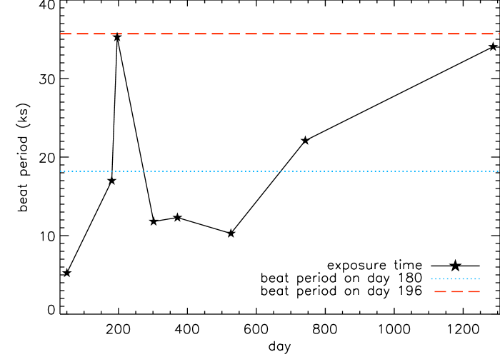
Figure 17: Illustration of detectability of two signals in our observations. The star symbols, connected by the black line, are the exposure times listed in Table 1. If the beat period between two signals is longer than the exposure time, then these frequencies can not be detected as two separate signals, because the exposure time does not cover at least one beat cycle. The blue dotted and red dashed lines indicate the beat periods for days 180 and 196. The limit imposed by too short exposure time prohibits the detection of these two frequencies on days 50, 301, 371, and 526. But for days 742 and 1286, at least the two frequencies found for day 180 would be detectable, unless the ratio of the amplitudes of the two signals is less than 1:2 for a 99.7% confidence detection (for a 95,4% and 90% confidence detection, an amplitude ratio of 1:3 and 1:4 is sufficient, respectively).

The superposition of two sine functions with different frequencies $f_{1}$ and $f_{2}$ results in beating at frequency $|f_{1}-f_{2}|$. We expect that two frequencies can only be separated with a given observation duration if it is longer than the beat period, $1/|f_{1}-f_{2}|$. The only observations for which we are able to find two frequencies are those on days 180 and 196. The difference between these two frequencies are 0.055 mHz and 0.028 mHz, respectively (see Table 7), and the expected beat periods are ($18.2\,\pm\,0.1$) ks and ($35.7\,\pm\,0.2$) ks, respectively. As can be seen from Table 1, the exposure times of these two observations are sufficiently long to cover one cycle of the beat period. However, the observations taken on days 301, 372, and 526 are significantly shorter, and two frequencies can not easily be separated. We tested this statement by analysing a synthetic light curve, sampled and noised as day 302 and modulated with two close frequencies of 0.72 and 0.76 mHz. Our 2-D method did not find a closed minimum within 3-$\sigma$ lines and the global minimum in the goodness contours is found for the combination of values of 0.678 and 0.745 mHz. Since the exposure times for days 371 and 526 are of the same order with lower signal to noise, we conclude that the exposure times for days 302, 371, and 526 are too short and the data are too noisy for a positive detection of two signals.

The importance of the exposure time for the resolution of two frequencies is illustrated in Fig. 17, where we plot the exposure times (in units ks) with the star symbols, connected by the black line and the beat periods for days 180 and 196 for comparison. The best resolving power can be achieved with the exposure times on days 196 and 1286 when a full beating cycle is covered. Two signals with a frequency difference as observed for days 180 or 196 can not be detected in any of the observations taken on days 50, 301, 371, and 526. However, the observation taken on day 742 was long enough to at least recover two frequencies if $|f_{2}-f_{1}|$ was as large as on day 180. For day 1286, the situation detected for day 196 would have been detectable. This conclusion is valid with comparable modulation amplitudes, but different amplitude ratios can affect the detectability. To test the effect, we have produced a synthetic data set sampled as day 742 and 1286, with amplitudes taken from Table 3 and with Poissonian noise. With our 2-D method, we were able to identify both signals at 0.72 and 0.76 mHz for the amplitude ratios 1:2, 1:3 and 1:4 at a confidence level of 99.7%, 95,4%, and 90%, respectively.

If on days 301, 372, and 526 the main peak was split in two signals as on days 180 or 196, then we would detect a value somewhere in between the minimum and maximum value. We experimented with synthetic light curves modulated by two signals of different amplitudes and found that the resultant frequency would be closer to the signal with the higher amplitude, and exactly in between if the amplitudes were the same. Meanwhile, the formal 3-$\sigma$ measurement uncertainties would be much smaller than the maximum frequency difference between two signals that could be detected with the given exposure times. As a consequence, the possibility of having detected an average frequency between two signals introduces a source of systematic uncertainty of the order of half the inverse exposure time, because this value limits the detectability of two signals.

It is noteworthy from Fig. 17 that the beat periods that correspond to the two signals on days 180 and 196 are suspiciously close to their respective exposure times. This similarity might raise suspicions that the exposure time could already predetermine the difference between the two signals. In the case of such a bias the same two frequencies would have resulted if the exposure times for days 180 and 196 had been the same. While we can not test longer exposure, we have run several tests using reduced exposure times for both light curves. For day 196 we only found a single frequency around 0.76 mHz if only the first 17 ks of the light curve are used. This can be explained by the reduced coverage of the beat period, and the detected two periods apparently require the long exposure time. Our analyses of a sample of reduced data sets for day 180 always resulted in two detected frequencies. The resulting values depend slightly on the selected subset of the light curve, but no correlation between effective exposure time and beat period is seen. The reason for the clear detection of two signals for day 180 can be seen in the well-pronounced sinusoidal form of the light curve with little contaminating noise, as can be seen from Fig. 8. The Lomb-Scargle method is limited by the requirement to cover at least one beating cycle in order to detect the respective two close signals (see Fig. 7). Meanwhile, our fitting approach is only limited by the quality of the data, and two close signals can be detected, even if only a fraction of the beating cycle is covered, if only the data have sufficient signal to noise. For day 196, the count rate is higher, but the light curve shows more irregular patterns, and a clear detection of two periods requires a more complete coverage of the beat period. From all these considerations we conclude that the presence of two frequencies is real in both cases and that the similarity between exposure time and beat period in the two cases must therefore be a coincidence.

4.4 Amplitudes

Figure 18: Normalised X-ray light curves for days 196, 302, 371, and 526 as indicated in the legends (solid lines) in comparison to day 180 (dotted line).

The comparison of normalised light curves in Fig. 18 illustrates that the oscillation amplitudes vary considerably between the observations. While only parts of the light curves are shown for better clarity, it is clear, e.g., from Figs. 1 and 8, that the amplitude of the first 10 ksec is representative for the full observation in each case. We include the normalised light curve for day 180 with a dotted line for reference. Clearly, on days 196 and 302, the relative amplitude was much smaller than on day 180, and it seems that it has almost recovered by day 372 but is smaller again on day 526.

The amplitude parameters, $A_{j}$ in Eq. 1, are representative of the evolution of the oscillation amplitude, as can be seen from, e.g., Figs. 8 and 15.

The evolution of the best-fit amplitude parameters $A_{j}$, relative to the mean count rates given in the last column of Table 1, is illustrated in Fig. 19. The values are listed in the last column of Table 3, where also the absolute amplitudes are given for each observation and each frequency. The absolute amplitudes have been determined directly from the detrended light curves before normalisation. In the bottom panel of Fig. 19 we show X-ray band fluxes (0.3-2.5 keV) for comparison. The description of flux measurements can be found in Sect.4.6. The sharp drop in brightness on day 180 first reported by Ness et al. (2003) can be identified in the bottom panel, and it coincides with a significant reduction in oscillation amplitude. While the brightness has completely recovered by day 196, the oscillation amplitudes remained low until the end of the SSS phase after day 526.

Table 3: Amplitude parameters $A_{j}$ from Eq. 1 for the days given in the first column. Given are the X-ray absolute amplitudes (in units counts per second, [cps]), and the X-ray amplitudes relative to the mean count rates given in the last column of Table 1, each for the respective frequencies $f_{j}$

Day	$f$ [mHz]	absolute [cps]	relative
50	0.760	$<0.047$	$<0.168$
180	0.719	$3.479\pm 0.190$	$0.099\pm 0.005$
	0.774	$5.465\pm 0.190$	$0.155\pm 0.005$
196	0.734	$0.967\pm 0.162$	$0.019\pm 0.003$
	0.762	$1.166\pm 0.163$	$0.022\pm 0.003$
302	0.744	$1.125\pm 0.235$	$0.032\pm 0.007$
371	0.721	$0.956\pm 0.158$	$0.054\pm 0.009$
526	0.726	$0.131\pm 0.082$	$0.035\pm 0.022$
742	0.749	$0.021\pm 0.008$	$0.237\pm 0.095$
1286	0.748	$0.009\pm 0.005$	$0.147\pm 0.094$

Figure 19: Top: Time evolution of the relative amplitudes $A_{j}$ listed in the last column of Table 3. Bottom: Evolution of X-ray fluxes (see Sect. 4.6) for comparison. The connection between the decline on day 180 and a sudden drop in relative amplitude can be recognised.

4.5 Other signals

Table 4: Significant detections of other X-ray frequencies in the range 0.6-0.9 mHz.

day	1st	2nd	3rd
180
$f\,[$mHz$]$	$0.628\pm 0.004$	$0.669\pm(0.006)^{a}$	$0.863\pm 0.004$
$A$(abs)	$0.777\pm 0.196$	$1.432\pm 0.193$	$1.991\pm 0.193$
$A$(rel)	$0.022\pm 0.006$	$0.041\pm 0.005$	$0.056\pm 0.005$
196
$f\,[$mHz$]$	$0.606\pm 0.004$	$0.703\pm 0.007$	$0.802\pm 0.004$
$A$(abs)	$0.693\pm 0.230$	$0.520\pm 0.232$	$0.586\pm 0.231$
$A$(rel)	$0.013\pm 0.004$	$0.010\pm 0.004$	$0.011\pm 0.004$
371
$f\,[$mHz$]$	–	$0.671\pm 0.030$	$0.870\pm 0.013$
$A$(abs)	–	$0.535\pm 0.179$	$0.692\pm 0.157$
$A$(rel)	–	$0.030\pm 0.010$	$0.039\pm 0.009$

^aunconstrained on 3-$\sigma$ level and only 2-$\sigma$ level given

While the focus of this paper is the substructure and evolution of the strongest signal around 0.75 mHz, other nearby signals are present. Leibowitz et al. (2006) found at least 12 significant frequencies for day 196, and for five of these, similar frequencies were also found for day 180. However, without uncertainty ranges it is difficult to decide whether or not these frequencies are related to each other.

In Table 4 we list all 3-$\sigma$ detections of frequencies in the range between 0.6 and 0.9 mHz for days 180-371. Basically, three significant frequencies can be detected in this range for days 180 and 196. Their values differ on a statistically significant level, and either these three frequencies are variable, or they occurred at random and are not related to each other. However, the two frequencies found for day 371 are both in good agreement with the corresponding frequencies on day 180, and these frequencies may have undergone a similar evolution as the main peak, i.e. reduction between days 180 and 196, followed by a slow increase back to the level seen on day 180. This is supported by the fact that the same trends of the third frequency in the last column of Table 4 can be seen as in Fig. 21. This behaviour could be related to the sharp decay that occurred on day 180. The beat periods between the main frequency of 0.75 mHz and the signals at 0.67 mHz and 0.87 mHz are both of order 10 ks, which is short enough to separate these frequencies from the main frequency, but too long in order to be detectable in the power spectrum. Along the definitions of amplitudes set out in Sect. 4.4, we calculated the relative and absolute amplitudes, which are also listed in Table 4.

Both, Ness et al. (2003) and Leibowitz et al. (2006) underlined the presence of overtones at $\sim 1.5$ mHz. We systematically searched for this signal in all data sets with the same techniques as described in the previous sections, and the results are presented in Table 5. The results from the Lomb-Scargle (L-S) and 2-D sine method agree well with each other. The dataset taken on day 50 is again too short to yield useful results within the 3-$\sigma$ contours, and the 1-$\sigma$ uncertainty range is given in round brackets. For days 180 and 196, we clearly detected two frequencies from both methods. The beat periods from the 2-D results are 17.8 and 19.6 ks, respectively, and such splitting of the main signal is thus detectable in the given observing durations (Table 1). We also found two frequencies in the day 742 observation with both techniques, yielding a beat period of $\sim 16$ ks. With the 2-D method, both frequencies are only significant on the 2-$\sigma$ level. For the other light curves, only a single frequency, if any, could be identified.

Table 5: First overtone X-ray frequencies expected around 1.5 mHz. For comparison, three linear combinations of the observed ground harmonics from the second column in Table 2 are given in the last three columns.

				Linear combinations of ground harmonics (Table 2):
Day	L-S	2-D sine fit	Leibowitz	$f_{1}+f_{2}$	$2\times f_{1}$	$2\times f_{2}$
			et al. (2006)	from 2-D sine fit	from 2-D sine fit	from 2-D sine fit
50	$(1.413)^{c}$	$1.401\,\pm\,(>0.100)^{a}$	–	–	$1.520\,\pm\,(>0.053)^{a}$	–
180	$1.485\,\pm\,0.018$	$1.491\,\pm\,0.009$	1.482	$1.493\,\pm\,0.005$	$1.438\,\pm\,0.004$	$1.548\,\pm\,0.003$
	$(1.562)^{c}$	$1.547\,\pm\,0.015$	–
196	$(1.460)^{c}$	$1.455\,\pm\,0.010$	1.459	$1.496\,\pm\,0.006$	$1.468\,\pm\,0.005$	$1.524\,\pm\,0.004$
	$(1.502)^{c}$	$1.506\,\pm\,0.008$	1.504
302	$(1.483)^{c}$	$1.478\,\pm\,0.044$	–	–	$1.488\,\pm\,0.012$	–
371	–	–	–	–	$1.442\,\pm\,0.011$	–
526	$(1.487)^{c}$	–	–	–	$1.452\,\pm\,0.028$	–
742	$(1.461)^{c}$	$1.461\,\pm\,(>0.016)^{b}$	–	–	$1.498\,\pm\,0.011$	–
	$(1.524)^{c}$	$1.522\,\pm\,(>0.017)^{b}$	–
1286	$(1.489)^{c}$	$1.489\,\pm\,0.037$	–	–	$1.496\,\pm\,0.011$	–

^aunconstrained on 3-$\sigma$ level and only 1-$\sigma$ level given
^bunconstrained on 3-$\sigma$ level and only 2-$\sigma$ level given
^cunconstrained on 1-$\sigma$ level and only the nominal value is given

The detected overtone frequencies listed in Table 5 need to be compared to the expected overtone frequencies based on the measured ground harmonics listed in Table 2, which are given in the last three columns, assuming the results from the 2-D sine fitting listed in the second column of Table 2. Expected overtones are those from $f_{1}+f_{2}$, $2\times f_{1}$, and $2\times f_{2}$. Within the combined uncertainties, all observed overtone frequencies can be uniquely associated to one of the expected overtone frequencies. The overtones determined from using the Lomb-Scargle algorithm are also in satisfactory agreement within the larger uncertainties. These findings are also in agreement with Leibowitz et al. (2006).

4.6 The X-ray spectra

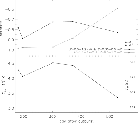
Figure 20: Parameterisation of the spectral evolution during the SSS phase. In the top panel, spectral hardness ratios with two different energy cuts, as detailed in the bottom right legend, are shown. In the bottom panel, best-fit colour temperatures derived from blackbody fits are shown, that show the same evolution as the hardness ratio curve plotted in black.

On order to compare our photometric results with the spectral evolution, we have extracted the high-resolution X-ray grating spectra taken during the SSS phase, thus on days 180, 196, 302, 371, and 526, using standard data reduction packages provided by the Chandra and XMM-Newton missions. For details on spectral analyses, we refer to, e.g., Ness et al. (2007). The SSS spectrum taken on day 180 has been shown in fig. 3 of Ness et al. (2003). We have also extracted the low-resolution spectra taken on day 50 with Chandra/ACIS and on days 742 and 1286 with XMM-Newton/MOS1.

From the spectra, we have determined X-ray band fluxes over the energy range 0.3-2.5 keV, which is covered by all instruments. For the high-resolution grating spectra, the fluxes can be obtained directly by integrating the photon energies from each spectral bin. The low-resolution spectra suffer from photon redistribution, but reliable fluxes can be obtained by fitting a spectral model to the data that is folded through the instrumental response matrix. The evolution of X-ray fluxes is shown in Fig. 19.

For the SSS spectra, we have determined the spectral colour for each spectrum, following two approaches. First, we computed two different hardness ratios $HR=(H-S)/(H+S)$ were $H$ and $S$ are the number of counts within a hard and a soft energy band, respectively. We computed two different hardness ratios from different energy cuts. The first hardness ratio has been computed with $0.35-0.5$ keV and $0.5-1.2$ keV for soft and hard bands, respectively, and a second one using the two bands $0.5-1.2$ keV and $1.2-3$ keV. In the top panel of Fig. 20, the evolution of the two hardness ratios is shown using a black and and a grey colour, as indicated in the bottom right legend. Clearly, the spectral evolution depends on the choice of the energy ranges.

We have therefore followed a second approach. As can be seen from fig. 3 in Ness et al. (2003), the shape of the SSS spectrum resembles that of an absorbed blackbody. Also other SSS spectra have a blackbody-like shape (see, e.g., fig. 4 in Ness et al. 2008 or fig. 4 in Ness et al. 2007). We have fitted absorbed blackbody models to each spectrum and obtained blackbody temperatures. While this quantity has the unit of a temperature, the values obtained from the spectral fits are most likely different from the effective temperature. It appears from previous work that blackbody temperatures derived from spectral fits to SSS spectra are systematically lower than the effective temperature, because the corresponding bolometric luminosity is unreasonably high (Krautter et al. 1996). The derived values can therefore not be considered more than a spectral characterisation. It is, however, one possibility that spectral changes are due to changes in the photospheric temperature. As we are interested in the temperature evolution, we assume that the evolution of the blackbody temperature reflects the evolution of the effective temperature. While this remains to be proven, we use this assumption as our working hypothesis.

In the bottom panel of Fig. 20 we show the evolution of the blackbody temperature. We have calculated statistical uncertainties accounting for correlations with other parameters, but these errors are smaller than the plot symbols. We caution, however, that a $\chi^{2}_{\rm red}$ goodness criterion indicates poor fits, and statistical errors are of little use in this situation. The reason for poor fits is the presence of deep absorption lines that are not reproduced by a blackbody. Since the continuum is well reproduced in each case, we still consider the blackbody fits a good approximation for the spectral shape. The best-fit blackbody temperatures are listed in Table 6. From day 180 to 196, the blackbody temperature decreases and recovers to a somewhat higher value on day 302. The temperature then stays approximately constant until day 371, after which time it decreases by a large amount. This behaviour resembles that of the evolution of the softer hardness ratio shown with the black line in the top panel of Fig. 20. The temperature decrease between days 180 and 196 may be associated to the steep decay on day 180, but it could also be an instrumental effect, as the spectrum on day 180 was taken with Chandra while that on day 196 was taken with XMM-Newton.

The normalisation can be converted to a radius assuming spherical geometry. With a distance of $d=3.9$ kpc, we obtain values ranging around 100,000 km. The bolometric luminosities that correspond to the derived temperatures and radii are two orders above the Eddington luminosity and must be considered unrealistically large. Consequently, the derived radius of $\sim 100,000$ km is overestimated and can be considered as upper limit.

5 Discussion

Figure 21: Graphical illustration of the evolution of the measured X-ray frequencies. The top panel shows the main frequency around 0.75 mHz, and in the bottom panel we show the first overtone. The bullets, connected by the solid line are the results from the 2-D method. The results from the Lomb-Scargle method are included with the dashed lines for comparison.

With a data set covering more than three years of evolution, we see large changes in brightness between observations. On day 180, a sharp decline was observed by Ness et al. (2003), and brightness variations thus occur on long and short time scales. The origin of the observed emission is not the same in all observations. On day 50, the X-ray emission likely originated from shocks within the ejecta, while on days 180-526, the spectrum was dominated by SSS emission that comes from the photosphere around the white dwarf. The post-SSS phase in novae is usually dominated by optically thin X-ray emission originating from the nebular ejecta that are radiatively cooling like in V382 Vel (see Ness et al. 2005). V4743 Sgr has a quiescent X-ray emission source (Ness et al. 2007) that could resemble those typically observed in intermediate polars, where X-ray emission originates from an accretion shock close to the white dwarf. In addition, Kang et al. (2006) detected a similar frequency of $0.7047\pm 0.0009$ mHz in optical observations which is likely associated with magnetically controlled accretion columns. The authors interpretted this frequency as the beating between the spin frequency of the white dwarf and the orbital modulation. Furthermore our optical/UV detection of a frequency of $0.699\pm 0.015$ mHz during day 742 is consistent with the Kang et al. (2006) optical finding within the errors. It thus stands to reason that the origin of the main X-ray frequency is of a fundamental nature as, e.g., the spin period of the white dwarf. However, systematic inspection of the frequency evolution yields some inconsistencies with the interpretation of pure rotational modulation.

We confirm the multifrequency substructure found by Leibowitz et al. (2006) for days 180 and 196. However, for day 180, we need the higher sensitivity of our 2-D sine fitting method, as the Lomb-Scargle method yields only a single peak. Similarly, Leibowitz et al. had to use a least square fitting approach in order to detect the double nature of the main peak for day 180. Since in addition, the formal measurement uncertainties from the Lomb-Scargle method are higher than for our 2-D sine fitting method, we concentrate only on the results from the 2-D sine fitting method for the discussion.

5.1 Evolution of the main frequency

The evolution of the main frequency is illustrated in Fig. 21. In the early observations, it is split in two frequencies, as the two signals on days 180 and 196 are different at $<99.7$% confidence. Since they have moved closer together from day 180 to day 196, it is possible that this was a monotonic trend that continued until they merged into a single frequency. Since the exposure times on days 301, 372, and 526 were much shorter than the beat period that corresponds to the difference between the two signals on day 180, this possibility can not be tested. However, as illustrated in Fig. 17, the observations on days 742 and 1286 were long enough to detect two frequencies if they were as far apart as on day 180. Unless the relative amplitudes of the two signals have changed significantly, we can confidently conclude for at least these two observations that only a single signal was present and that the double nature of the 0.75-mHz signal has disappeared. These results are also supported by the overtone studies. The detected values satisfy the characteristics of a fundamental and a first harmonic.

After day 196, the frequency appears to have decreased and then increased again by day 742 (see Fig. 21). While this is formally not statistically significant in the 3-$\sigma$ level, other nearby signals have undergone such kind of change on a statistically significant level (see Table 4). Furthermore, the decrease of the relative amplitude as illustrated in Fig. 19 is highly significant. In addition to being split in two nearby frequencies in the early evolution, the main frequency is thus not a stable signal.

In spite of the likely different origin of the optical emission observed by Kang et al. (2006), they found a similar period to our main frequency, yielding $0.7047\,\pm\,0.0009$ mHz, which is consistent with our optical/UV measurements obtained with XMM-Newton OM on day 742. While their frequency is remarkably close to our main X-ray frequency, the statistical uncertainty ranges indicate a significant difference from all our measurements (see Table 2), including the late observations up to 1286 days after outburst. Nevertheless, the similarity of the frequency is striking and suggests some fundamentally common underlying origin. However, if the spin period of the white dwarf were to be responsible for the modulations in X-ray and optical, then the frequencies in both bands should be identical.

The fact that the optical and the X-ray frequencies differ, plus the obvious changes in frequency and amplitude, demonstrate that there is more than simply rotational modulation from the spin of the white dwarf.

5.2 Pulsations versus Spin Modulation

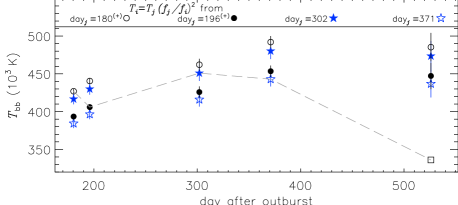
Figure 22: Graphical illustration of the connection between changes in X-ray frequency and colour temperature. Each data point represents a predicted temperature $T_{i}$ for each observation taken at time day_i after outburst (x-axis), according to the formula given in the top, where $T_{j}$ is the blackbody temperature (see Sect. 4.6) for day_j as indicated by the plot symbol (see legend), and $f_{j}/f_{i}$ is the ratio of frequencies from our measurements. The dashed grey line represents the observed colour temperatures (see Fig. 20) for comparison with the predictions (the symbols that are connected by this line are the cases $i=j$, thus the measured temperatures).

While Kang et al. (2006) rule out pulsations, the new evidence from our analysis requires us to reopen the case. Kang et al. argued that the interpretation of this period as white dwarf pulsations would yield a significant slow-down with time, owing to cooling of the temperature of the white dwarf (Somers & Naylor 1999). From their estimates of changes in effective temperature, derived from observed luminosity changes, they calculated that the period reported by Ness et al. (2003) for day 180 should be 38 minutes around day 1000, and they rule out pulsations because no such period is in their data. While it is true that we are also not observing a 38 minute period in the X-ray data around day 1000, we do see significant frequency changes in Fig. 21.

Kang et al. (2006) suggested using equation 10 in Kjeldsen & Bedding (1995) for the conversion of temperature changes to expected pulsation frequency changes. In Sect. 4.2 of Kjeldsen & Bedding (1995), a scaling relation between stellar parameters and pulsation frequencies is derived. It is argued that the acoustic cut off frequency, $\nu_{\rm max}$, that defines a typical time scale of the atmosphere, scales with the maximum envelope frequency of stellar pulsations. Linear adiabatic theory is applied to derive $\nu_{\rm max}$ and thus the relation given in their equation 10. The ratio of two pulsation frequencies in two different atmospheres scales with the square root of the inverse ratio of the respective effective temperatures (assuming the same mass and radius). With this method, our observed changes in frequency can be converted to expected changes in photospheric temperature, if pulsations were assumed. In Table 6 we list squared ratios of frequencies from our 2-D sine fitting method taken from Table 2. We indicate the two respective observation dates with numbers (1) and (2) for which the ratios were taken. For days 180 and 196 we indicate the high and low frequencies by superscript ’+’ and ’-’ behind the day of observation. Since the 3-$\sigma$ uncertainties given in Table 6 do not include the possibility that two unresolved frequencies are present, we used the larger uncertainty range resulting from half of the inverse exposure times for days 302, 371, and 526. The inverse exposure time sets a strict limit on the detectability of two separate frequencies (see Sect. 4.3 and Fig. 17), and if the signal was split in two components on days 302, 371, and 526, then a value somewhere in between would result (depending on the individual amplitudes), while the statistical uncertainty would not include the upper or lower frequency.

As an estimate of the evolution of the effective temperature, we use colour temperatures derived in Sect. 4.6. As pointed out earlier, the blackbody temperature is not equivalent to the photospheric temperature, and also the evolution might not follow the same trend. However, we consider it a strong possibility that changes in the blackbody temperature indicate equivalent changes in temperature and assume this as a working hypothesis. The following conclusions depend on whether or not this assumption is valid.

In the last three columns of Table 6 we quote the colour temperatures derived in Sect. 4.6 for the respective days and the inverse ratios of these values for direct comparison with the squared frequency ratios in the third column. The extent of agreement between these ratios is an indicator for the validity of the underlying assumption of pulsations. Those ratios which agree within the given uncertainty ranges of the frequency measurement are indicated by underlined numbers. For illustration we show in Fig. 22 the evolution of the observed colour temperature in comparison with temperatures computed from

$$T_{i}=T_{j}*(f_{j}/f_{i})^{2}\,,$$ (3)

where $T_{i}$ and $f_{i}$ are predicted temperature and observed frequency for day_i, respectively, and $T_{j}$ and $f_{j}$ are the observed temperature and frequency for day_j.

The best agreement between observed and predicted effective temperature is seen for the observations on days 180 and 302, and between days 196 and 371. All predictions derived from day 526 are far off the mark and are not included in the plot. This can be seen from the predictions from other observations for day 526, which are too high, indicating that the frequency changes do not predict the decline in temperature. The agreement between predicted and observed temperature between days 196 and 302 and between days 180 and 196 is poorer. In light of the underlying assumptions made by Kjeldsen & Bedding (1995), a main sequence (MS) stars with an effective temperature of order 5500 K, plus the considerable uncertainty in the effective temperature, the agreements are surprisingly good, strongly suggesting that pulsations play an important role. The breakdown of the relationship towards the end of the SSS phase can be understood as the turn off of the central energy source, leading to a highly non-equilibrium situation, and pulsations may not propagate the same way as in equilibrium. We thus argue that the possibility of pulsations can at least not easily be ruled out.

It must be noted that for a frequency of $\sim 0.75$ mHz and a mass of order 0.5-1.4 M_⊙, equation 10 of Kjeldsen & Bedding (1995) yields effective radii of order 2-7 R_⊙, which appears rather large for a hot WD and is about an order of magnitude larger than the radii derived in Sect. 4.6 from blackbody fits, which have been discussed to be unrealistically large. If this apparent discrepancy could be resolved by a larger scaling factor, then the relative changes of effective temperature and oscillation changes would still hold for a hot white dwarf. Without computing new models for hot white dwarfs, the validity of the relation must be taken with care. However, if we assume this relation to be valid, then we have good reason to conclude that pulsations are occurring between days 180 and 371.

A fact that complicates the interpretation is the similarity between the frequencies measured during the SSS phase and during the last phase, long after the nova has turned off. This similarity suggests that a fundamentally similar origin is accountable, which brings us back to the spin period of the white dwarf. While pulsations seem to be a valid explanation for the SSS phase, the spin period of the white dwarf should also play a major role. We have no explanation but hesitate to believe in a coincidence. Perhaps magnetic fields that are present in an intermediate polar might stir up the ejecta during the SSS phase and stimulate pulsations. However, this is pure speculation.

Leibowitz et al. (2006) interpreted the 0.75 mHz structure as due to the rotation of the white dwarf and other close signals as the nonradial pulsations of the central star. This explanation would be consistent with a similar interpretation by Drake et al. (2003) and Rohrbach et al. (2009) for the nova V1494 Aql. A dominant short-term oscillation with a period of 2498.9 s with other close signals was detected. The authors interpreted the variability as the pulsations of the central white dwarf. These central acretors after the nova explosion resemble planetary nebula nuclei where pulsations were observed in the range of $\sim 1000$ s to $\sim 5000$ s (Ciardullo & Bond 1996). For example, the white dwarf in the planetary nebula NGC 246 had a principal frequency of 0.67 mHz in September 1989 and 0.54 mHz in June 1990 (Ciardullo & Bond 1996). This gives a change of 0.13 mHz within 9 months, i.e., $\sim 0.01$ mHz per month. This is remarkably similar to our finding of changes in each of the two frequencies detected on days 180 and 196 (Table 2), which change by the amount of $\sim 0.01$ mHz within two weeks. Such frequency changes are thus not unprecedented in pulsating white dwarfs.

Sastri & Simon (1973) studied instabilities in hydrogen burning nova shells and found pulsations as a possible phenomenon. However, while the multiperiodic and unstable behaviour is consistent with our results, the predicted typical periods are much smaller. For example, the unstable 35 s X-ray oscillations in RS Oph (Beardmore et al. 2008) shortly after the start of the super soft phase would fall into this range.

Another mechanism with periods in accordance to our finding could be pulsations in isolated hot GW Vir white dwarfs. The origin of these pulsations is the compression-induced opacity and ionisation increase in the partial ionisation zones of carbon and oxygen (Starrfield et al. 1984). Such nonradial pulsations are typical for hydrogen-deficient white dwarfs with carbon-oxygen envelopes. While in accreting white dwarfs like V4743 Sgr the white dwarf is not hydrogen poor on its surface, Dreizler et al. (1996) found some GW Vir stars that have pulsations and hydrogen on their surface. The X-ray spectra of V4743 Sgr contain relatively deep carbon and oxygen absorption lines (Ness et al. 2003), which is an indication for V4743 Sgr being a CO-type nova as opposed to an ONe-type nova. Drake et al. (2003) proposed the same interpretation in the case of the nova V1494 Aql, but without any spectral indication of the white dwarf to be the required CO type.

Table 6: Comparison of squared X-ray frequency ratios (frequencies from 2-D method from Table 2) with inverse ratios of colour temperature ($T_{\rm col}$ in $10^{3}$ K, derived in Sect. 4.6. For days 180 and 196, the low and high frequencies are marked with - and + superscripts, respectively. The errors include systematic uncertainties from the exposure times (see text for details). The underlined numbers indicate cases for which the relation $(f_{1}/f_{2})^{2}\simeq T_{\rm col}^{(2)}/T_{\rm col}^{(1)}$ holds. Note that mismatches involve only days 196 and 526, times of non-equilibrium situations (see Sect. 5.2).

Day(1)	Day(2)	$(f_{1}/f_{2})^{2}$	$T_{\rm col}^{(1)}$	$T_{\rm col}^{(2)}$	$T_{\rm col}^{(2)}/T_{\rm col}^{(1)}$
180-	196-	0.96$\,\pm\,0.01$	427	406	0.95
180+	196+	$1.03\,\pm\,0.01$	427	406	0.95
196-	302	$0.97\,\pm\,0.11$	406	451	1.11
196+	302	1.05$\,\pm\,0.11$	406	451	1.11
302	371	1.06$\,\pm\,0.16$	451	443	0.98
371	526	$0.99\,\pm\,0.17$	443	336	0.76
180+	302	1.08$\,\pm\,0.11$	427	451	1.06
180+	371	1.15$\,\pm\,0.12$	427	443	1.04
180+	526	$1.14\,\pm\,0.13$	427	336	0.79
302	526	$1.05\,\pm\,0.17$	451	336	0.74

5.3 Connection between spin and orbital period

Leibowitz et al. (2006) and Kang et al. (2006) argued that the two nearby frequencies can arise from the white dwarf spin period on the one hand and the beat period between the spin and the orbital period of the binary system on the other hand. The orbital period was reliably determined by Kang et al. (2006) as $6.718\,\pm\,0.005$ hours from both observing campaigns. This can be compared to the beat periods between various pairs of observed frequencies. In Table 7 we list the detected periods in minutes, the difference between their frequencies, and the derived beat periods. We calculated the beat periods for the two signals in the X-ray light curves taken on days 180 and 196 (top two rows), for all possible combinations between these two signals and the optical period of 23.651 min (derived from the $f_{1}=0.7047$ mHz frequency found by Kang et al. (2006); following four rows), and the combinations of periods observed in the late X-ray light curves and the optical period (bottom two rows).

The beat periods between the two periods detected on days 180 and 196 are clearly inconsistent with the orbital period. Also, the beat periods between these frequencies and the optical frequency are not consistent with the orbital period. Only the beat periods between the frequencies derived from the late X-ray observations and the optical frequency are in agreement with the orbital period. The latter agreement suggests that either the optical or the late X-ray period is the spin period, while the respective other one is the beat between orbital and spin period. The most probable situation is that the X-ray signal is the spin of the white dwarf. The fact that none of the earlier frequencies are connected to the orbit-spin relation, lends additional support to our interpretation that the oscillations during the SSS phase are more than only the spin period of the white dwarf.

Table 7: Beat periods $P_{\rm beat}$ (last column in unit hours), derived from various pairs of observed periods ’$P_{1}$’ and ’$P_{2}$’ (in unit minutes) and their corresponding frequencies, $f_{1}$ and $f_{2}$. In the top two rows, the beat periods for the two close frequencies that we found in the X-ray light curves on days 180 and 196 (see Table 2) are given. Next, the beat period between each X-ray period and optical period of 23.651 minutes, observed between days 1003 and 1011 by Kang et al. (2006), are given. The last two rows show the beat period between the late X-ray periods and the optical period, which compare well to the orbital period of 6.72 hours.

Day	$P_{1}$ [min]	$P_{2}$ [min]	$f_{2}$ - $f_{1}$ [mHz]	$P_{\rm beat}$ [h]
180	$23.180$	$21.533$	$0.055\,\pm\,0.005$	$5.1\,\pm\,0.5$
196	$22.707$	$21.872$	$0.028\,\pm\,0.006$	$9.9\,\pm\,2.2$
180	$23.180$	$23.652^{a}$	$0.069\,\pm\,0.003$	$4.0\,\pm\,0.2$
180	$21.533$	$23.652^{a}$	$0.014\,\pm\,0.004$	$19.8\,\pm\,6.2$
196	$22.707$	$23.652^{a}$	$0.057\,\pm\,0.004$	$4.9\,\pm\,0.3$
196	$21.872$	$23.652^{a}$	$0.029\,\pm\,0.005$	$9.6\,\pm\,1.7$
742	$22.252$	$23.652^{a}$	$0.044\,\pm\,0.011$	$6.3\,\pm\,1.7$
1286	$22.282$	$23.652^{a}$	$0.043\,\pm\,0.011$	$6.4\,\pm\,1.8$

^aDetected optical period between days 1003 and 1011 ($f_{2}=0.7047\pm 0.0009$ mHz)

5.4 The coincidence between pulsation and spin modulation

In Sect. 5.2 we have discussed that during the SSS phase, the main period could be characterised by pulsations, while the frequency detected in the later observations is more likely the spin period of the white dwarf. In that case we wonder why the frequencies are so similar, despite of their different nature (see, e.g., Fig. 6).

We consider it unlikely that the spin period of the white dwarf has changed, yet small but significant changes in the observed oscillation frequency are undeniable. We can only speculate about how to explain the presence of a persistent signal that is variable at the same time. Perhaps, the spin period of the white dwarf could be modulated by additional processes that could depend on the physical conditions of the emitting plasma. One possibility would be that the magnetic field axis is not aligned with the rotation axis, and the spinning of the non-aligned magnetic dipole stirs up the ejecta surrounding the white dwarf. In this way pulsations could be stimulated by the spin period of the white dwarf. The flux is then modulated by these pulsations and the time evolution would depend on the properties of the ejecta. We also note that the expansion of the shell during the SSS phase that rotates at a slower velocity in the outer layers, owing to conservation of angular momentum, could slow down the oscillation frequency. We caution, however, that these ideas are unsubstantiated without theoretical support and are as such highly speculative.

5.5 The decline on day 180

In Figs. 19 and 21 it can be seen that the largest changes in frequency and amplitude as well as the shrinking difference between the two components of the main peak appeared shortly after the sudden brightness decline on day 180 that was accompanied by spectral changes from soft optically thick to hard optically thin (Ness et al. 2003). Since this decline has only been seen in the first SSS observation, thus during the early SSS phase, it may be part of an early variability phase similar to that first seen by Swift in RS Oph (e.g., Beardmore et al. 2008). Such an early variability phase is now routinely being observed, e.g., in V458 Vul (see figure 6 in Ness et al. 2009). Since these novae did not show any persistent oscillations as in V4743 Sgr, our findings are a unique contribution to the discussion about the origin of the early variations in the SSS phase. Additional evidence comes from high-resolution spectroscopy. Ness (2010, in preparation) reports the rapid disappearance of some of the nebular emission lines that were seen during the dark phase (Ness et al. 2003). This indicates that the surrounding nebular emission was recombining after the bright central X-ray source had disappeared. One possibility for the complete disappearance of the X-ray source could be an expansion of the photospheric radius, followed by photospheric adjustment, thus shifting the peak of the SED back into the ultraviolet. This would be consistent with the spectral changes parameterised in Fig. 20. From day 180 to day 196, a significant drop in the blackbody temperature and hardness is seen which could indicate a lower photospheric temperature on day 196. In that case, the atmospheric structure could change significantly, which could lead to changes in pulsation frequency and amplitude, as the conditions for the propagation of pulsations through the atmosphere would change. Our observations of changes in the oscillations are important evidence for a physical explanation of the variations rather than geometrical causes such as an eclipse.

6 Summary

In this paper, all available X-ray light curves of the nova V4743 Sgr are presented and analysed. Our results have to be viewed in light of three different phases of evolution, each with a different origin of X-ray emission:

• Early hard X-ray emission phase with X-rays likely originating from shocks within the ejecta. This phase is characterised by weak emission line spectra that can be modeled with optically thin thermal models. Our observation taken on day 50 belongs to this phase.

• Super Soft Source (SSS) phase with the X-ray emission originating from a pseudo photosphere around the white dwarf. This phase is characterised by extremely bright continuum emission. The broad-band spectrum can be fitted by a blackbody, and high-resolution X-ray spectra show absorption lines that are blue shifted (see Ness et al. 2009). Our observations taken on days 180, 196, 302, 371, and 526 belong to this phase.

• Quiescent phase. In Classical novae, the radiatively cooling ejecta can be observed in X-rays. The spectra from days 742 and 1286 resemble more those of quiescent intermediate polars (Ness et al. in prep).

Despite of all the differences in the emission origin, the same main frequency was observed at all times. In addition, a similar frequency was observed in the optical (Kang et al. 2006 and our XMM-Newton optical/UV OM data), although the optical light has a different origin. If the optical period is interpreted as the beat period between the WD spin and the orbit, then the optical light must originate from something fixed in the orbiting system, for example from the secondary star or the disc-stream impact region. Not many periodic processes in a cataclysmic variable can leave their footprint in all forms of light, leading us to the conclusion that the spin period of the white dwarf must play a major role.

Meanwhile, the different phases can lead to different kinds of modulation of the main frequency, and we have investigated small anomalies that require detailed analysis. Our main results are:

• On days 180 and 196, the main signal consists of two nearby frequencies. The difference between these two components shrinks from day 180 to day 196. While only a single frequency was found for days 302 to 526, these observations were too short to detect such close signals. Either, the trend of a shrinking difference has continued until it merged into a single signal, or roughly the same difference has remained through the SSS phase.

• The observations of days 742 and 1286 contained only a single signal, and the double nature has not continued into the quiescent phase.

• The average frequency decreased slightly after day 196 and then increased again after day 526. Colour temperatures derived in Sect. 4.6 from fits to the SSS spectra on days 180, 302, and 371, seem to change in relation to the changes in frequency. This suggests pulsations as an origin for the modulations.

• The relative amplitude of the oscillations decreased after day 196 and then increased again to the original value after day 526.

• The largest change in frequency and oscillation amplitude occurred after the sudden brightness decline on day 180 and could thus be connected to this event.

• We found overtones at $\sim 1.5$ mHz in the periodograms of all observations, which are first harmonics and combinations of two close fundamentals present near the main feature at $\sim 0.75$ mHz.

• The beat period between the X-ray period and the optical period during the quiescent phase coincides with the orbital period.

We believe that during the SSS phase, pulsations are the major source for the oscillations, while the oscillations seen during the quiescent phase are the spin period of the white dwarf. The similarity of the spin period and pulsation period is puzzling, and no mechanism that could co-align the periods is known to us. Based on the spin period, we support the interpretation by Kang et al. (2006) that V4743 Sgr is an intermediate polar.

References

- Beardmore et al. (2008) Beardmore A. P., Osborne J. P., Page K. L., Goad M. R., Bode M. F., Starrfield S., 2008, in A. Evans, M. F. Bode, T. J. O’Brien, & M. J. Darnley ed., Astronomical Society of the Pacific Conference Series Vol. 401 of Astronomical Society of the Pacific Conference Series, Swift-XRT Discovery of a 35s Periodicity in the 2006 Outburst of RS Ophiuchi. p. 296
- Bode & Evans (2008) Bode M. F., Evans A., 2008, Classical Novae
- Brinkman et al. (2000) Brinkman B. C., Gunsing T., Kaastra J. S., et al. 2000, in J. E. Truemper & B. Aschenbach ed., Society of Photo-Optical Instrumentation Engineers (SPIE) Conference Series Vol. 4012 of Society of Photo-Optical Instrumentation Engineers (SPIE) Conference Series, Description and performance of the low-energy transmission grating spectrometer on board Chandra. pp 81–90
- Ciardullo & Bond (1996) Ciardullo R., Bond H. E., 1996, AJ , 111, 2332
- Drake et al. (2003) Drake J. J., Wagner R. M., Starrfield S., Butt Y., Krautter J., Bond H. E., Della Valle M., Gehrz R. D., Woodward C. E., Evans A., Orio M., Hauschildt P., Hernanz M., Mukai K., Truran J. W., 2003, ApJ , 584, 448
- Dreizler et al. (1996) Dreizler S., Werner K., Heber U., Engels D., 1996, A&A , 309, 820
- Haseda et al. (2002) Haseda K., West D., Yamaoka H., Masi G., 2002, IAUC , 7975, 1
- Horne & Baliunas (1986) Horne J. H., Baliunas S. L., 1986, ApJ , 302, 757
- Kang et al. (2006) Kang T. W., Retter A., Liu A., Richards M., 2006, AJ , 132, 608
- Kato et al. (2002) Kato T., Fujii M., Ayani K., 2002, IAUC , 7975, 2
- Kjeldsen & Bedding (1995) Kjeldsen H., Bedding T. R., 1995, A&A , 293, 87
- Krautter et al. (1996) Krautter J., Oegelman H., Starrfield S., Wichmann R., Pfeffermann E., 1996, ApJ , 456, 788
- Leibowitz et al. (2006) Leibowitz E., Orio M., Gonzalez-Riestra R., Lipkin Y., Ness J., Starrfield S., Still M., Tepedelenlioglu E., 2006, MNRAS , 371, 424
- Morgan et al. (2003) Morgan G. E., Ringwald F. A., Prigge J. W., 2003, MNRAS , 344, 521
- Ness et al. (2009) Ness J., Drake J. J., Beardmore A. P., et al. 2009, AJ , 137, 4160
- Ness et al. (2008) Ness J., Schwarz G., Starrfield S., Osborne J. P., Page K. L., Beardmore A. P., Wagner R. M., Woodward C. E., 2008, AJ , 135, 1328
- Ness et al. (2007) Ness J., Schwarz G. J., Retter A., Starrfield S., Schmitt J. H. M. M., Gehrels N., Burrows D., Osborne J. P., 2007, ApJ , 663, 505
- Ness et al. (2007) Ness J., Starrfield S., Beardmore A. P., Bode M. F., Drake J. J., Evans A., Gehrz R. D., Goad M. R., Gonzalez-Riestra R., Hauschildt P., Krautter J., O’Brien T. J., Osborne J. P., Page K. L., Schönrich R. A., Woodward C. E., 2007, ApJ , 665, 1334
- Ness et al. (2003) Ness J., Starrfield S., Burwitz V., Wichmann R., Hauschildt P., Drake J. J., Wagner R. M., Bond H. E., Krautter J., Orio M., Hernanz M., Gehrz R. D., Woodward C. E., Butt Y., Mukai K., Balman S., Truran J. W., 2003, ApJL , 594, L127
- Ness et al. (2005) Ness J., Starrfield S., Jordan C., Krautter J., Schmitt J. H. M. M., 2005, MNRAS , 364, 1015
- Nielbock & Schmidtobreick (2003) Nielbock M., Schmidtobreick L., 2003, A&A , 400, L5
- Nousek et al. (1987) Nousek J. A., Garmire G. P., Ricker G. R., Collins S. A., Reigler G. R., 1987, Astrophysical Letters Communications, 26, 35
- Petz et al. (2005) Petz A., Hauschildt P. H., Ness J., Starrfield S., 2005, A&A , 431, 321
- Rohrbach et al. (2009) Rohrbach J. G., Ness J., Starrfield S., 2009, AJ , 137, 4627
- Sastri & Simon (1973) Sastri V. K., Simon N. R., 1973, ApJ , 186, 997
- Scargle (1982) Scargle J. D., 1982, ApJ , 263, 835
- Somers & Naylor (1999) Somers M. W., Naylor T., 1999, A&A , 352, 563
- Starrfield et al. (1984) Starrfield S., Cox A. N., Kidman R. B., Pesnell W. D., 1984, ApJ , 281, 800
- Talavera (2009) Talavera A., 2009, Astrophys. Space Sci. , 320, 177
- Turner et al. (2001) Turner M. J. L., Abbey A., Arnaud M., et al. 2001, A&A , 365, L27
- van den Heuvel et al. (1992) van den Heuvel E. P. J., Bhattacharya D., Nomoto K., Rappaport S. A., 1992, A&A , 262, 97