Continuum and line modelling of discs around young stars
I.  300 000 disc models for Herschel/GASPS

Abstract

We have combined the thermo-chemical disc code ProDiMo with the Monte Carlo radiative transfer code Mcfost to calculate a grid of $\sim$300 000 circumstellar disc models, systematically varying 11 stellar, disc and dust parameters including the total disc mass, several disc shape parameters and the dust-to-gas ratio. For each model, dust continuum and line radiative transfer calculations are carried out for 29 far IR, sub-mm and mm lines of [OI], [CII], ¹²CO and o/p-H₂O under 5 inclinations. The grid allows to study the influence of the input parameters on the observables, to make statistical predictions for different types of circumstellar discs, and to find systematic trends and correlations between the parameters, the continuum fluxes, and the line fluxes. The model grid, comprising the calculated disc temperature and chemical structures, the computed SEDs, line fluxes and profiles, will be used in particular for the data interpretation of the Herschel open time key programme GASPS. The calculated line fluxes show a strong dependence on the assumed UV excess of the central star, and on the disc flaring. The fraction of models predicting [OI] and [CII] fine-structure lines fluxes above Herschel/Pacs and Spica/Safari detection limits are calculated as function of disc mass. The possibility of deriving the disc gas mass from line observations is discussed.

1 Introduction

The structure, composition and evolution of protoplanetary discs are important corner-stones to unravel the mystery of life, as they set the initial conditions for planet formation. Spectral energy distributions (SEDs), although their analysis is known to be degenerate, probe the amount, temperature and overall geometry of the dust in the discs, such as disc flaring (Meeus et al., 2001), puffed-up inner rims (Dullemond et al., 2001; Acke et al., 2009), and indications of an average grain growth in discs as young as a few Myr (D’Alessio et al., 2001).

Most works in the past decade have focused on the analysis of SEDs of individual objects (e.g. D’Alessio et al., 2006) or to study systematic trends in infrared colours of various types of discs, ranging from embedded young stellar objects to exposed T Tauri stars (Robitaille et al., 2006). Some ambiguities inherent in SED analysis can be resolved by images in scattered light (Stapelfeldt et al., 1998), in mid-infrared thermal emission (McCabe et al., 2003) or in the mm-regime (Andrews & Williams, 2007). The Spitzer observatory has enabled detailed studies on dust mineralogy, constraining dust properties in the upper layers of the inner disk regions by using solid-state features (Furlan et al., 2006; Olofsson et al., 2009). Multi-technique, panchromatic approaches, combining the aforementioned observations, are now becoming possible but remain limited to a few objects with complete data sets (e.g. Wolf et al., 2003; Pinte et al., 2008; Duchene et al., 2009).

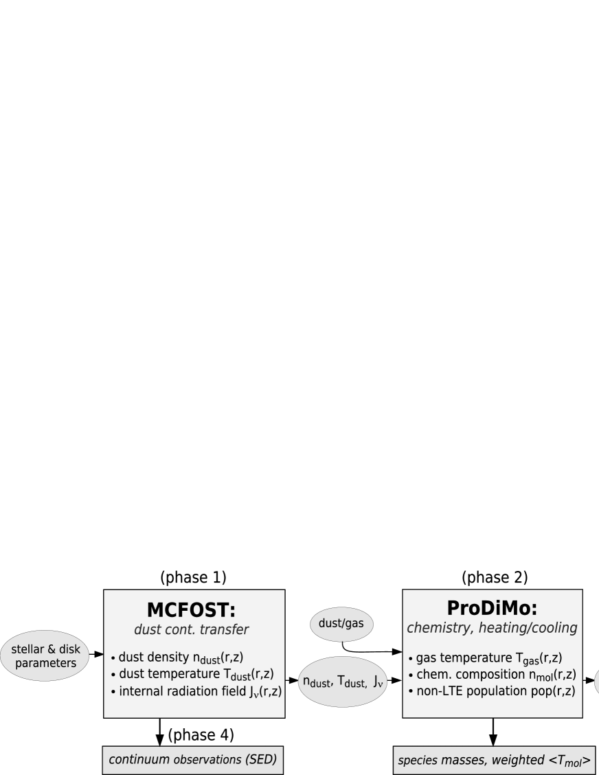
Figure 1: Unified Mcfost / ProDiMo model pipeline to calculate one radiation thermo-chemical disc model with SED and line flux prediction.

However, all these observational findings are related to the dust component. Initially, about 99% of the disc mass can be assumed to be present in form of gas, and the progress toward a better understanding of the gas component, such as chemical composition, gas temperature structure and vertical disc extension, is hampered by a current lack of observational data. With several key programs of the Herschel Space Observatory, such as GASPS and WISH, a new body of gas emission line observations will be provided very soon, and there is a clear need to include the gas in such systematic studies. Recent work has focused on the prediction of far IR line emissions from individual discs (Meijerink et al., 2008; Ercolano et al., 2008; Woitke et al., 2009; Cernicharo et al., 2009), or rather small parameter studies (Kamp et al., 2009). Goicoechea & Swinyard (2009) have recently discussed the detection rates of the $\rm[OI]\,63\,\mu$m, $\rm[SI]\,56\,\mu$m and $\rm[SiII]\,34\,\mu$m fine-structure lines with Herschel and the proposed Spica/Safari mission on the basis of one low mass disc model ($M_{\rm gas}\!=\!10^{-5}\rm\,M_{\odot}$) by Gorti & Hollenbach (2004). Their conclusions, however, depend on the choices of the other model parameters, and it is difficult to put them on a firm statistical basis.

To address these issues, we have combined our state-of-the-art computer codes to calculate the dust and line radiative transfer with the Mcfost-code (Pinte et al., 2006), and the gas thermal balance and chemistry with the ProDiMo-code (Woitke et al., 2009; Kamp et al., 2009). We have computed a large grid of 300 000 disc models to simultaneously predict SEDs and gas emission lines from parametrised disc density distributions. The grid name DENT stands for Disc Evolution with Neat Theory. The following sections describe the model pipeline (Sect. 2) and the first results on fine structure emission line fluxes and detectability (Sect. 3). Section 4 summarises the preliminary findings of the DENT grid and provides an outlook to future studies.

2 The DENT grid

The DENT grid is a tool to investigate the influence of stellar, disc and dust properties (Table 1) on continuum and line observations (Table 2), and to study in how far these dependencies can be inverted. The grid is designed to coarsely sample the parameter space associated with young, intermediate to low-mass stars at ages (1-30 Myr) having gas-rich and gas-poor discs.

Table 1: Parameters of the DENT grid and values assumed. $R_{\rm subli}$ stands for the dust sublimation radius (where ${T_{\rm d}}\!=\!1500\,$K). The choice of inclination angles resembles a randomly oriented sample.

stellar parameter
$M_{\star}$	stellar mass $[M_{\odot}]$	0.5, 1.0, 1.5, 2.0, 2.5
$age$	age [Myr]	1, 3, 10, 100
$f_{\rm UV}$	excess UV $f_{\rm UV}\!=\!L_{UV}/L_{\star}$	0.001, 0.1
disc parameter
$M_{\rm d}$	disc dust mass $[M_{\odot}]$	$10^{-7}$, $10^{-6}$, $10^{-5}$, $10^{-4}$, $10^{-3}$
$\rho_{\rm d}/\rho_{\rm g}$	dust/gas mass ratio	0.001, 0.01, 0.1, 1, 10
$R_{\rm in}$	inner disc radius $[R_{\rm subli}]$	1, 10, 100
$R_{\rm out}$	outer disc radius [AU]	100, 300, 500
$\epsilon$	column density $N_{\rm H}(r)\propto r^{\displaystyle-\epsilon}$	0.5, 1.0, 1.5
$H_{0}$	scale height [AU]	fixed: 10 @ $r_{0}\!=\!100$AU
$\beta$	disc flaring $H(r)=H_{0}\big{(}\frac{r}{r_{0}}\big{)}^{\displaystyle\beta}$	0.8, 1.0, 1.2
dust parameter
$a_{\rm min}$	minimum grain size $[\mu m]$	0.05, 1
$a_{\rm max}$	maximum grain size $[\mu m]$	fixed: 1000
$s$	settling $H(r,a)\propto H(r)\;a^{\displaystyle-s/2}$	0, 0.5
inclination angle
$i$	$0^{o}$ (face-on), $41.4^{o}$, $60^{o}$, $75.5^{o}$, $90^{o}$ (edge-on)

Table 2: List of output quantities: monochromatic continuum fluxes $F_{\rm cont}$ and integrated, continuum-subtracted line fluxes $F_{\rm line}$.

observable	wavelengths [$\mu$m]
$F_{\rm cont}$	57 $\lambda$-points between $0.1\mu$m and $3500\mu$m
OI	63.18, 145.53
CII	157.74
12CO	2600.76, 1300.40, 866.96, 650.25, 520.23, 433.56, 371.65,
	325.23, 289.12, 260.24, 144.78, 90.16,79.36, 72.84
o-H2O	538.29, 179.53, 108.07, 180.49, 174.63, 78.74
p-H2O	269.27, 303.46, 100.98, 138.53, 89.99, 144.52

In the DENT grid, 11 variable and 2 fixed input parameters (see Table 1) are required to specify the star + disc systems. The input stellar parameters are mass and age. The corresponding effective temperatures and luminosities are from the evolutionary models of Siess et al. (2000). For the photospheric spectra, we use Kurucz stellar atmosphere models of solar abundance and matching $T_{\rm eff}$ and $\log(g)$. Because some young stars show significant accretion and/or chromospheric activity, an extra UV component is added to the spectrum in DENT. This extra UV component has an important impact on the disc chemistry and temperature. It is defined as $f_{\rm UV}\!=\!L_{\rm UV}/L_{\star}$ where $L_{\rm UV}\!=\!\int_{\rm 91\,nm}^{\rm 250\,nm}L_{\lambda}\,d\lambda$ is the UV luminosity with assumed spectral shape $L_{\lambda}\!\propto\!\lambda^{0.2}$.

There are other sources of energy in the discs. The interstellar irradiation is assumed to be isotropic and fixed throughout the grid by (Eq. 27 of Woitke et al., 2009, with $\chi^{\rm ISM}\!\!=\!1$). The cosmic ray ionisation rate of H₂ is set to $\zeta_{\rm CR}\!=\!1.7\!\times\!10^{-17}\rm\,s^{-1}$. We further assume that all discs are passive, i.e. there is no viscous heating. This will have an impact on the inner structure and temperature of some discs. However, the SED of several sources in the literature are well fitted without viscous heating, e.g. IM Lupi (Pinte et al., 2008) and IRAS 04158+2805 (Glauser et al., 2008).

The density structure of the disc is parametric, with power-laws used for the surface density, the scale height, and the dust size distribution. Optical properties of astronomical silicate (Draine & Lee, 1984) are used to calculate the dust opacities.

The chemical abundances are calculated selecting 9 atomic elements, 66 molecular and 5 ice species, 950 reactions, and element abundances as outlined in (Woitke et al., 2009). The numerical code used here feature an improved coupling between the UV radiative transfer and the calculation of the UV photo-rates (see Kamp et al., 2009). This version of DENT does not contain PAHs. This will have an impact in particular on the Herbig AeBe’s, with a possible increase of the gas temperature, especially in the upper layers of the discs. We do not expect a significant effect on the continuum. The role of PAHs will be explored in a forthcoming paper.

To calculate the DENT grid, two numerical codes were used in a sequence that we now describe (see Fig. 1). In phase 1, Mcfost solves the dust radiative transfer problem to obtain the dust temperature structure $T_{\rm d}(r,z)$ and the internal mean intensities $J_{\nu}(r,z)$. In phase 2, these data are transferred to ProDiMo which calculates the gas temperature structure $T_{\rm g}(r,z)$ assuming gas thermal balance, the chemical composition $n_{\rm mol}(r,z)$ assuming kinetic chemical equilibrium, and the level population of the gas species in the disc. An escape probability method is used to calculate the level populations. Phase 2 requires an additional gas parameter: the dust-to-gas ratio, $\rho_{\rm d}/\rho_{\rm g}$. Among the results of phase 2 are the total species masses $M_{\rm mol}$ and averaged gas temperatures $\langle T_{\rm g}^{\rm mol}\rangle$ for $\rm mol\!\in\!\{O,C^{+},CO,H_{2}O\}$, defined as

$$\langle T_{\rm g}^{\rm mol}\rangle \!\!=\!\! \frac{\int n_{\rm mol}(r,z)\,T_{\rm g}(r,z)\;dV}{\int n_{\rm mol}(r,z)\;dV}\ ,$$ (1)

where $n_{\rm mol}(r,z)$ is the particle density at position $(r,z)$ in the disc. In phase 3, the level populations are transferred back to Mcfost to calculate the emission line profiles. The formal line transfer solutions are computed in 301 velocity bins on $100\!\times\!72$ parallel rays organised in log-equidistant concentric rings in the image plane. A Keplerian rotation velocity field is assumed for the bulk disk kinematics, and a thermal $\!+\!$ turbulent broadening with $v_{\rm turb}\!=\!0.15\,$km/s is added. The calculations are completed by phase 4 running formal solutions of the dust continuum radiative transfer problem on the same rays. The calculated continuum and line intensities are post-processed to get the integrated line fluxes after continuum subtraction. Further details are listed in Table 2.

In total, the DENT grid comprises 323020 disc models and SED calculations. A total number of 1610150 line flux calculations have been carried out for 29 spectral lines under 5 inclinations. We note that some parameter combinations may lead to unrealistic models, but they have been kept for the sake of completeness.

3 Results

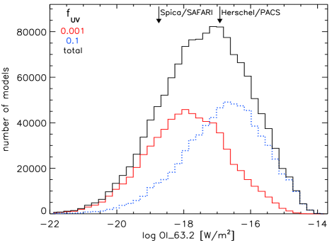
Figure 2: Dependence of line flux [OI] 63.2$\mu$m on the stellar UV excess $f_{\rm UV}$. The black histogram counts the DENT models that result in certain [OI] 63.2$\mu$m fluxes at distance 140pc in 40 log-equidistant bins. The red histogram represents the low $f_{\rm UV}\!=\!0.001$ models, and the blue dotted histogram the high $f_{\rm UV}\!=\!0.1$ models. The difference between high and low UV excess causes a difference of about $1-1.5$ orders of magnitude in line flux. The arrows show the $(3\sigma,0.5h)$ detection limits of Spica/Safari and Herschel/Pacs, see dependence on disc mass in Table 3.

Figure 2 depicts all calculated line fluxes of $\rm[OI]\,63.2\,\mu$m in form of 3 histograms, underlining the depending on the assumed stellar UV excess. Models with high $f_{\rm UV}$ (blue in the figure) have warm disc surfaces heated by the stellar UV with ${T_{\rm g}}\!\gg\!{T_{\rm d}}$, and hence strong emission lines. Models with low $f_{\rm UV}$ (red) have gas temperatures more equal to the dust temperatures, and hence less strong emission lines. The dependence of $F_{\rm line}$ on $f_{\rm UV}$ is significant for all stars (also in other lines), but is less pronounced for Herbig Ae/Be stars which already produce photospheric soft UV, even for $f_{\rm UV}\!=\!0$. For example, a Kurucz stellar atmosphere model with $T_{\rm eff}\!=\!8500\,$K, $\log(g)\!=4$ attains $L_{\rm UV}\!\approx\!0.097L_{\star}$ whereas a model with $T_{\rm eff}\!=\!4500\,$K, $\log(g)\!=4$ only attains $L_{\rm UV}\!\approx\!2\cdot 10^{-6}L_{\star}$. Table 3 lists the fraction of models predicting line fluxes of [OI] and [CII] larger than (0.5h , 3$\sigma$) detection limits of Herschel/Pacs and Spica/Safari at 140pc as function of disc gas mass. Note that, for massive discs, the line emitting regions may be optically thick in the continuum and may have $T_{\rm g}\!\approx\!T_{\rm d}$. In such cases, there is only very limited contrast between line and continuum, leaving a fair fraction of massive discs with non-detectable lines.

Table 3: Fraction of DENT models predicting line fluxes larger than (0.5h , 3$\sigma$) detection limits of Herschel/Pacs and Spica/Safari at 140pc as function of total disc gas mass $M_{\rm gas}\rm\,[M_{\odot}]$ and stellar UV excess $f_{\rm UV}$. Each entry in this table is based on more than 5000 disc models. We neglect detection problems due to background confusion here.

${}_{f_{\rm UV}}$ \ ${}^{M_{\rm gas}}$	$10^{-7}$	$10^{-6}$	$10^{-5}$	$10^{-4}$	$10^{-3}$	$10^{-2}$	$10^{-1}$
$|F_{\rm[OI]63.2\mu{\rm m}}|>1.2\!\times\!10^{-17}\rm\,W/m^{2}$ (Herschel/Pacs)
0.1	0%	20%	51%	66%	70%	71%	71%
0.001	0%	6%	17%	23%	26%	30%	34%
$|F_{\rm[OI]145.5\mu{\rm m}}|>4\!\times\!10^{-18}\rm\,W/m^{2}$ (Herschel/Pacs)
0.1	0%	0%	9%	30%	45%	52%	57%
0.001	0%	0%	3%	7%	12%	18%	23%
$|F_{\rm[CII]157.7\mu{\rm m}}|>4\!\times\!10^{-18}\rm\,W/m^{2}$ (Herschel/Pacs)
0.1	0%	0%	17%	52%	56%	57%	56%
0.001	0%	0%	6%	14%	14%	14%	13%
$|F_{\rm[OI]63.2\mu{\rm m}}|>1.8\!\times\!10^{-19}\rm\,W/m^{2}$ (Spica/Safari)
0.1	65%	90%	96%	95%	96%	97%	96%
0.001	38%	65%	79%	83%	86%	86%	85%
$|F_{\rm[OI]145.5\mu{\rm m}}|>1.2\!\times\!10^{-19}\rm\,W/m^{2}$ (Spica/Safari)
0.1	5%	44%	68%	80%	85%	87%	88%
0.001	1%	15%	29%	46%	56%	62%	63%
$|F_{\rm[CII]157.7\mu{\rm m}}|>1.2\!\times\!10^{-19}\rm\,W/m^{2}$ (Spica/Safari)
0.1	0%	83%	95%	94%	95%	94%	93%
0.001	0%	53%	81%	78%	76%	73%	69%

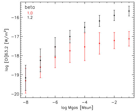
Figure 3: Dependence of line flux of [OI] 63.2$\mu$m at distance $d\!=\!140\,$pc on the flaring parameter $\beta$, as function of total disc gas mass $M_{\rm gas}$. A sub-selection of 3456 T Tauri models is plotted ($M_{\star}\!\leq\!1\rm\,M_{\odot}$, $age\!\leq\!1\rm\,Myr$, $f_{\rm UV}\!=\!0.1$, $R_{\rm in}\!=\!R_{\rm subli}$, $s\!=\!0$, inclination angle $\leq\!60^{o}$, where the statistical range of line flux predictions due to the variation of the other input parameters in expressed by mean values and standard deviations.

Another clear trend in the models is depicted in Fig. 3, which shows the calculated line fluxes of $\rm[OI]\,63.2\,\mu$m for a sub-selection of T Tauri disc models with high $f_{\rm UV}$ as function of disc mass. At low disc masses, the discs are optically thin and the flaring of the disc (see definition of $\beta$ in Table 1) has only little influence on the line fluxes. However, with increasing disc mass, the inner disc becomes optically thick and the computed line fluxes split up into two branches. For strong flaring ($\beta\!=\!1.2$), the fluxes of the emission lines steadily increase further, whereas for non-flaring discs ($\beta\!\leq\!1$) they saturate at $M_{\rm gas}\!\approx\!10^{-5}-10^{-4}\rm\,M_{\odot}$, henceforth called the “saturation disc mass”. In other words, for massive T Tauri discs, high far IR line fluxes (e.g. $\rm[OI]\,63.2\,\mu m\!\ga\!3\times 10^{-17}\,W/m^{2}$) are a safe indicator of disc (gas) flaring. In flared geometry, the disc surface is directly heated by the star, hence higher temperatures and stronger emission lines. In non-flared geometry, the surface layers are situated in the shadow casted by the dust in the inner disc regions, and the gas temperatures are cooler. In that case, a further increase in disc mass does not lead to stronger emission lines, but rather to an increase of the shielding effects, causing cooler temperatures and sometimes even weaker emission lines.

The saturation behaviour of the emission lines for non-flared geometry depends on the line properties. High-excitation lines like $\rm[OI]\,145.5\,\mu$m react more sensitively to temperature changes and hence to disc flaring, whereas low excitation lines like CO $J$=1$\to$0, $\rm[CII]\,157.7\,\mu$m are less affected. However, the point where these saturation effects start to appear, the saturation disc mass, is found to be rather similar for all lines, because it is the amount of dust and its opacity in the inner disc regions that causes the shielding.

The fact that different emission lines originate in different disc regions, and the strong dependencies of the line fluxes on UV excess $f_{\rm UV}$ and flaring index $\beta$ suggest that a simple, PDR-like analysis of emission line ratios to determine the total disc mass is difficult. However, Fig. 4 shows that most of these complicated parameter dependencies affect the line fluxes in an indirect way, namely by changing the mean temperature of the disc. If we plot the dependency between disc gas mass and $\rm[OI]63.2\mu$m line flux for models with similar mean disc temperatures, we roughly retrieve a linear relation as expected from a simple analysis (see Appendix A).

The $1\sigma$ errorbars in Fig. 4 show, however, that there is still a considerable variation of the $\rm[OI]63.2\mu$m flux among the models, even if they have similar mean disc temperatures. Note also, that the fitting value of $T_{\rm exc}\!=\!30.5$K is not consistent with the actual disc temperatures as measured from the models. This may be due to the way we have defined the mean disc temperature (Eq. 1) and/or due to included non-LTE effects. Kamp et al. (2009) have shown that, in general, $T_{\rm exc}<T_{\rm g}$ in the outer and upper disc layers.

We note that an unmindful usage of Eq. (4) with an assumed value for $T_{\rm exc}$ (e.g. 27K) for the purpose of gas mass determination from a measured $\rm[OI]63.2\mu$m line flux can be misleading and does not account for the variety of results that we find in the DENT model grid. In particular, high mass discs tend to be cooler as demonstrated by the saturation behaviour depicted in Fig. 3, and their oxygen fine-structure lines can easily become optically thick.

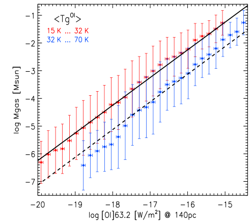
Figure 4: Relation between total disc gas mass and $\rm[OI]\,63.2\mu$m line flux at distance 140pc. The $x$-axis is subdivided into 30 log-equidistant bins. In each bin, the values of the disc gas mass (parameter, see Table 1) of all models with matching $\rm[OI]\,63.2\mu$m line flux are statistically analysed to yield a mean value and a standard variation, which are then plotted as points with vertical error bars. We distinguish between cool and warm models by $\langle T_{\rm g}^{\rm OI}\rangle$ as defined in Eq. (1), and have chosen temperature interval boundaries to bracket the $1\sigma$ distribution as shown by the inserted histogram. The following models have been selected: dust/gas ratio $\rho_{\rm d}/\rho_{\rm g}\!=\!0.01-1$, flaring index $\beta\!\geq\!1$, and inclination angle $\leq\!60^{o}$, altogether 122269 cool and 101244 warm models. The full and dashed lines show the results from the formula Eq. (4) with $T_{\rm exc}\!=\!24$K and $T_{\rm exc}\!=\!30.5$K, respectively.

4 Summary and Conclusions

In a concerted effort of the theory groups in Edinburgh, Grenoble and Groningen, we have computed a grid of 300 000 circumstellar disc models, simultaneously solving gas-phase, UV-photo and ice chemistry, detailed heating & cooling balance, and continuum & line radiative transfer.

The first results of the DENT grid show a strong dependence of the calculated emission line fluxes on the assumed stellar UV excess and on the flaring of the disc. The stellar UV is essential for the heating of the upper disc layers. In combination with positive disc flaring, a strong stellar UV irradiation creates an extended warm surface layer with ${T_{\rm g}}\!>\!{T_{\rm d}}$ responsible for the line emissions. However, if the disc is not flared (self-shadowed), discs with total mass $\ga\!10^{-5}-10^{-4}\rm\,M_{\odot}$ increasingly shield the stellar UV by their inner parts, which causes much cooler surface layers, and a saturation of the line fluxes with increasing disc mass.

Despite these complicated parameter dependencies, we have shown that the $\rm[OI]\,63.2\mu$m line flux depends basically on two quantities, namely the total disc gas mass and the mean disc temperature. We will continue this work by two follow-up papers (Kamp et al. 2010, in prep., Ménard et al. 2010, in prep.) that will provide more insight into the statistical behaviour of gas line and dust continuum predictions, respectively, to identify trends and robust correlations with disc mass.

In summary, the DENT grid allows to

$\bullet$	study the effects of stellar, disc, and dust parameters on continuum and line observations,
$\bullet$	allow for a qualified interpretation of observational data,
$\bullet$	quickly predict line and continuum fluxes for planning observations,
$\bullet$	search for best-fitting models concerning a given set of observed line and continuum fluxes,
$\bullet$	study the robustness of certain fit values against variation of the observational data.

We intend to make the calculated DENT grid available to the scientific community. A graphical user interface called xDENT has been developed to allow researchers to visualise the DENT results, to make plots as presented in this letter, and to search for best-fitting models for a given set of continuum and line flux data. We emphasise, however, that the DENT grid has not been developed for detailed fitting of individual objects. The coarse sampling of the 12-dimensional parameter space can mostly be used to narrow down the parameter range for individual objects, for example to design a finer sub-grid, especially for not so well-known objects.

With a comprehensive data set of far IR gas emission lines to be obtained by Herschel/GASPS very soon, we aim at breaking the degeneracy of SED fitting and make possible a more profound analysis of the physical, chemical and temperature structures of discs around young stars.

Appendix A Simple line emission model

Let us assume that an emission line is optically thin and that the emitting species is populated with a uniform excitation temperature $T_{\rm exc}$. The line luminosity is then given by

$$L_{\rm line}=h\nu\,A_{ul}\,N_{\rm tot}\frac{g_{u}\exp(-E_{u}/kT_{\rm exc})}{Q(T_{\rm exc})}\ ,$$ (2)

where $\nu$ is the line centre frequency, $A_{ul}$ is the Einstein coefficient of the line transition from level $u$ to level $l$, $Q$ is the partition function, and $g_{u}$ and $E_{u}$ are the statistical weight and energy [K] of the upper level. The total number of line emitting particles $N_{\rm tot}$ is related to the total disc gas mass by

$$N_{\rm tot}=\epsilon N_{\langle H\rangle}=\epsilon\,\frac{M_{\rm gas}}{\mu_{H}}\ ,$$ (3)

where $\epsilon$ is the abundance of the line emitting species with respect to hydrogen nuclei and $\mu_{H}\!\approx\!1.31\,$amu the gas mass per hydrogen nucleus, assuming solar abundances.

The observable line flux $\rm[erg/s/cm^{2}]$ at distance $d$ is

$$F_{\rm line}=\frac{L_{\rm line}}{4\pi\,d^{2}}\ .$$ (4)

For the case of the $\rm[OI]\,63.2\mu$m fine-structure line, we have $u\!=\!2$, $l\!=\!1$, $A_{21}\!=\!8.87\times 10^{-5}\rm\,s^{-1}$, $E_{2}\!=\!227.7\,$K, $g_{1}\!=\!5$ and $g_{2}\!=\!3$. We calculate the partition function including the third level $E_{3}\!=\!326.0\,$K, $g_{3}\!=\!1$. The oxygen abundance assumed in the models is $\epsilon\!=\!8.5\times 10^{-4}$. However, the actual abundance of the neutral oxygen atom is reduced by CO, CO-ice, H₂O and H₂O-ice formation, and we use a mean value from the models, $\epsilon\!=\!3.6\times 10^{-4}$.

References

- Acke et al. (2009) Acke B., Min M., van den Ancker M. E., Bouwman J., Ochsendorf B., Juhasz A., Waters L. B. F. M., 2009, A&A, 502, L17
- Andrews & Williams (2007) Andrews S. M., Williams J. P., 2007, ApJ, 659, 705
- Cernicharo et al. (2009) Cernicharo J., Ceccarelli C., Ménard F., Pinte C., Fuente A., 2009, ApJL, 703, L123
- D’Alessio et al. (2001) D’Alessio P., Calvet N., Hartmann L., 2001, ApJ, 553, 321
- D’Alessio et al. (2006) D’Alessio P., Calvet N., Hartmann L., Franco-Hernández R., Servín H., 2006, ApJ, 638, 314
- Draine & Lee (1984) Draine B. T., Lee H. M., 1984, ApJ, 285, 89
- Duchene et al. (2009) Duchene G., McCabe C., Pinte C., Stapelfeldt K. R., Menard F., Duvert G., Ghez A. M., Maness H. L., Bouy H., Barrado y Navascues D., Morales-Calderon M., Wolf S., Padgett D. L., Brooke T. Y., Noriega-Crespo A., 2009, ApJ, accepted
- Dullemond et al. (2001) Dullemond C. P., Dominik C., Natta A., 2001, ApJ, 560, 957
- Ercolano et al. (2008) Ercolano B., Drake J. J., Raymond J. C., Clarke C. C., 2008, ApJ, 688, 398
- Furlan et al. (2006) Furlan E., Hartmann L., Calvet N., D’Alessio P., Franco-Hernández R., Forrest W. J., Watson D. M., Uchida K. I., Sargent B., Green J. D., Keller L. D., Herter T. L., 2006, ApJS, 165, 568
- Glauser et al. (2008) Glauser A. M., Ménard F., Pinte C., Duchêne G., Güdel M., Monin J., Padgett D. L., 2008, A&A, 485, 531
- Goicoechea & Swinyard (2009) Goicoechea J. R., Swinyard B., 2009, astro-ph 0909.3280
- Gorti & Hollenbach (2004) Gorti U., Hollenbach D., 2004, ApJ, 613, 424
- Kamp et al. (2009) Kamp I., Tilling I., Woitke P., Thi W., Hogerheijde M., 2009, astro-ph 0911.1949
- McCabe et al. (2003) McCabe C., Duchêne G., Ghez A. M., 2003, ApJL, 588, L113
- Meeus et al. (2001) Meeus G., Waters L. B. F. M., Bouwman J., van den Ancker M. E., Waelkens C., Malfait K., 2001, A&A, 365, 476
- Meijerink et al. (2008) Meijerink R., Glassgold A. E., Najita J. R., 2008, ApJ, 676, 518
- Olofsson et al. (2009) Olofsson J., Augereau J., van Dishoeck E. F., Merín B., Lahuis F., Kessler-Silacci J., Dullemond C. P., Oliveira I., Blake G. A., Boogert A. C. A., Brown J. M., Evans II N. J., Geers V., Knez C., Monin J., Pontoppidan K., 2009, A&A, 507, 327
- Pinte et al. (2006) Pinte C., Ménard F., Duchêne G., Bastien P., 2006, A&A, 459, 797
- Pinte et al. (2008) Pinte C., Padgett D. L., Ménard F., Stapelfeldt K. R., Schneider G., et al. 2008, A&A, 489, 633
- Robitaille et al. (2006) Robitaille T. P., Whitney B. A., Indebetouw R., Wood K., Denzmore P., 2006, ApJS, 167, 256
- Siess et al. (2000) Siess L., Dufour E., Forestini M., 2000, A&A, 358, 593
- Stapelfeldt et al. (1998) Stapelfeldt K. R., Krist J. E., Menard F., Bouvier J., Padgett D. L., Burrows C. J., 1998, ApJL, 502, L65
- Woitke et al. (2009) Woitke P., Kamp I., Thi W., 2009, A&A, 501, 383
- Woitke et al. (2009) Woitke P., Thi W., Kamp I., Hogerheijde M. R., 2009, A&A, 501, L5
- Wolf et al. (2003) Wolf S., Padgett D. L., Stapelfeldt K. R., 2003, ApJ, 588, 373