High Energy Bounds on Soft ${\cal N}\!=\!4$ SYM Amplitudes from AdS/CFT

Abstract:

Using the AdS/CFT correspondence, we study the high-energy behavior of colorless dipole elastic scattering amplitudes in ${\cal N}\!=\!4$ SYM gauge theory through the Wilson loop correlator formalism and Euclidean to Minkowskian analytic continuation. The purely elastic behavior obtained at large impact-parameter $L$, through duality from disconnected $AdS_{5}$ minimal surfaces beyond the Gross-Ooguri transition point, is combined with unitarity and analyticity constraints in the central region. In this way we obtain an absolute bound on the high-energy behavior of the forward scattering amplitude due to the graviton interaction between minimal surfaces in the bulk. The dominant “Pomeron” intercept is bounded by $\alpha\leq{11}/7$ using the AdS/CFT constraint of a weak gravitational field in the bulk. Assuming the elastic eikonal approximation in a larger impact-parameter range gives $4/3\leq\alpha\leq{11}/7.$ The actual intercept becomes $4/3$ if one assumes the elastic eikonal approximation within its maximally allowed range $L\gtrsim\exp{Y/3},$ where $Y$ is the total rapidity. Subleading AdS/CFT contributions at large impact-parameter due to the other $d=10$ supergravity fields are obtained. A divergence in the real part of the tachyonic KK scalar is cured by analyticity but signals the need for a theoretical completion of the AdS/CFT scheme.

1 Introduction

From the point of view of the microscopic theory, the problem of high-energy soft ($i.e.$, at small transverse momentum transfer) hadronic elastic amplitudes has yet remained essentially unsolved. Indeed, it involves the non perturbative regime of the underlying Quantum Chromodynamics field theory (QCD) at strong coupling, which, apart from lattice calculations, is beyond reach at the moment. However, some fundamental properties have been known since a long time, coming from the $S$-matrix formalism, and they are expected to hold for a consistent quantum field theory. They are Unitarity, coming from the conservation of probabilities, and Analyticity. These properties, combined with the existence of a “mass gap” in the asymptotic particle spectrum, lead to the celebrated Froissart bound for the total cross section [1, 2, 3], which corresponds (up to logarithms) to an intercept not greater than $1$ for the leading Regge singularity, usually called the “Pomeron”. To be more precise, in terms of the impact-parameter ($\vec{b}$) and rapidity ($Y$) dependence of the partial elastic amplitude $a(Y,\vec{b})$, unitarity gives a bound on ${\rm Im}\ a\leq 2$ (in standard units), while confinement provides a bound on the impact-parameter radius $L\propto Y.$ Both ingredients enter the derivation of the Froissart bound.

Recently, a new tool for dealing with soft amplitudes has appeared, namely the Gauge/Gravity duality, whose precise realization has been first found [4, 5, 6, 7] within the formalism of the AdS/CFT correspondence. Generally speaking, Gauge/Gravity duality is expected to relate a strongly coupled gauge field theory with a “weakly coupled” 5-dimensional supergravity limit of a 10-dimensional string theory. This raises the hope to find a solution by mapping high-energy amplitudes into supergravity by duality. In the realization of the AdS/CFT correspondence, the gauge theory is the ${\cal N}=4$ supersymmetric Yang-Mills (SYM) gauge theory, which is a conformal field theory and thus non-confining: the result should then differ from what is found in a confining theory like QCD. However, attacking the problem of soft amplitudes in this context may be a useful laboratory for further developments in QCD. Indeed, the study of soft high-energy scattering amplitudes in ${\cal N}=4$ SYM using the AdS/CFT correspondence, and more generally Gauge/Gravity duality, has attracted much attention in the literature [8, 9, 10, 11, 12, 13, 14, 15, 16, 17, 18, 19, 20, 21, 22, 23, 24, 25].

In the conformal case there is no mass gap, and thus the Froissart bound is not expected to be valid for ${\cal N}=4$ SYM theory. However, unitarity and analyticity are still expected to hold, and so it is interesting to examine the question of high-energy bounds in this context. Indeed, in the perspective of applying the same tools to gauge theories more similar to QCD, it is worthwhile to learn more from the precise “laboratory” furnished by the AdS/CFT correspondence. For this sake we shall use together unitarity, analyticity and the AdS/CFT correspondence to give a precise account of soft high-energy elastic amplitudes in the ${\cal N}=4$ supersymmetric gauge theory.

The difficult problem one is faced with when using the AdS/CFT correspondence is that it applies to the planar, large-$N_{c}$ limit of the gauge theory. This planar approximation corresponds to purely elastic contributions since there is no particle production, and so it does not take into account the contribution of inelastic multiparticle channels, which are an essential feature for determining soft high-energy amplitudes. However, the analytic continuation from Euclidean to Minkowskian space may generate inelasticity for the scattering amplitude (see Ref. [9, 10]).

Our guideline is to circumvent this difficulty by combining the knowledge one can obtain from AdS/CFT in the region of applicability of the supergravity approximation, $i.e.$, the large impact-parameter region where the amplitude is essentially elastic, with the constraints coming from analyticity and unitarity which are expected to hold for gauge field theories.

To be specific we shall consider the following ingredients:

• The rôle of massive quarks and antiquarks ($Q,\bar{Q}$) in the AdS/CFT correspondence will be played, as in [26, 27], by the massive $W$ bosons arising from breaking $U(N+1)\rightarrow U(N)\times U(1),$ where one brane is considered away from the $N\to\infty$ others. Hence, the role of hadrons will be devoted to “onia” defined as linear combinations of $Q\bar{Q}$ colorless “dipole” states [28, 29, 30, 31] of average transverse size $\langle{|\vec{R}|}\rangle$, which sets the scale for the onium mass.

• The dipole amplitudes will be defined through correlators of Wilson loops in Euclidean space, in order to avoid the complications of the Lorentzian AdS/CFT correspondence (see $e.g.$ [32]). Hence, we will start from the Euclidean formulation of the problem, and then perform an analytic continuation [33, 34, 35, 36, 37, 38, 39] to obtain the physical quantity in Minkowski space [40, 41, 42, 43, 44].

• The AdS/CFT correspondence will allow to relate the calculation of the Euclidean Wilson loop correlator to a minimal surface problem in the Anti de Sitter bulk, which has been solved [8] at large impact-parameter distance $L$ using the knowledge of (quasi-)disconnected minimal surfaces, connected by supergravity fields propagating in the bulk. This is the solution of the minimal surface problem beyond the Gross-Ooguri transition point [45, 46].

• After analytic continuation, this result will lead to an estimate of cross sections and elastic amplitudes at large impact parameter. Combined with unitarity and analyticity to fix a bound in the lower impact-parameter domain, it will lead to a determination of new energy bounds on the forward elastic amplitudes, or, equivalently, on the total cross sections in ${\cal N}=4$ SYM .

Note that we base our analysis on the use of minimal surface solutions in AdS space with Euclidean signature [8, 9, 10]. More recently, the use of minimal surfaces in AdS space with Minkowskian signature for two- and many-body gluon scattering has been developed (see [47, 48] and references therein). In the present work we stick to the study of soft scattering amplitudes for colorless states.

The plan of the paper is as follows. In section 2, we formulate the amplitudes in terms of Wilson loop correlators in Euclidean space, where the AdS/CFT correspondence is applied, and we define properly the analytic continuation to the physical Minkowski space. In section 3 we derive the formulation of the AdS/CFT minimal surface solution [8] for the impact-parameter dependent amplitudes valid at large impact-parameter (extended to unequal dipole sizes). In the following section 4, the impact-parameter domain for the applicability of the AdS/CFT correspondence is determined from the weak gravitational field constraint in the AdS dual. Together with unitarity constraints it allows us, in section 5, to determine an absolute bound on the high-energy behavior of total cross sections and thus on the leading “Pomeron” intercept of the forward elastic amplitude. We briefly discuss subleading contributions, among which the next-to-leading, parity-odd one corresponds to the “Odderon” in ${\cal N}\!=\!4$ SYM theory. In section 6, we summarize our main results, compare them with existing studies and propose an outlook on future related studies.

2 Elastic amplitudes from Euclidean Wilson Loop correlators

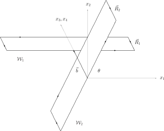
Figure 1: Geometry of the Wilson loops in Euclidean space. The transverse kinematic variables ($\vec{b},\vec{R}_{1,2})$ remain unchanged by the analytic continuation to Minkowski space, while $\theta\to-i\chi$, see text.

In order to obtain information on high-energy elastic scattering amplitudes at strong coupling, we will follow the approach of [8] to evaluate them through the Gauge/Gravity correspondence, making use of minimal surfaces in the gravity bulk. The specific tool we will use is the AdS/CFT correspondence, which allows to evaluate a certain Wilson-loop correlation function in ${\cal N}=4$ SYM theory in Euclidean space through its gravitational dual, together with analytic continuation into the physical Minkowski space, where this correlator corresponds to a dipole-dipole elastic scattering amplitude. In this Section we briefly describe the Wilson loop formalism [40, 41, 42, 43, 44], and the analytic continuation required to relate Euclidean and Minkowskian quantities [33, 34, 35, 36, 37, 38, 39].

In the eikonal approximation, dipole-dipole elastic scattering amplitudes in the high energy limit and at small momentum transfer (the so-called soft high-energy regime) can be conveniently expressed in terms of the normalized connected correlator ${\cal C}_{M}$ of Wilson loops in Minkowski space [41, 42, 43, 44]

$${\cal A}(s,t;\vec{R}_{1},\vec{R}_{2}) =-2is\int d^{2}\vec{b}\,e^{i\vec{q}\cdot\vec{b}}\,{\cal C}_{M}(\chi,\vec{b};\vec{R}_{1},\vec{R}_{2})$$ (1)

$$\equiv-2is\int d^{2}\vec{b}\,e^{i\vec{q}\cdot\vec{b}}\left\langle{\frac{{\cal W}_{1}{\cal W}_{2}}{\left\langle{{\cal W}_{1}}\right\rangle\left\langle{{\cal W}_{2}}\right\rangle}-1}\right\rangle,$$

where $t=-\vec{q}^{\,2}$, $\vec{q}$ being the transverse transferred momentum (here and in the following we denote with $\vec{v}$ a two-dimensional vector), and the Wilson loops follow the classical straight-line trajectories for quarks (antiquarks, in parenthesis) [49]:

$${\cal W}_{1}\longrightarrow X^{\mu}=b^{\mu}+u_{1}^{\mu}\tau\,(+r_{1}^{\mu})\ ;\quad\quad{\cal W}_{2}\longrightarrow X^{\prime\mu}=u_{2}^{\mu}\tau\,(+r_{2}^{\mu})\ .$$ (2)

Here $u^{\mu}_{1,2}$ are unit time-like vectors along the directions of the momenta defining the dipole classical trajectories, and moreover $b^{\mu}=(0,0,\vec{b})$ and $r^{\mu}_{1,2}=(0,0,\vec{R}_{1,2}).$ The loop contours are then closed at positive and negative infinite proper-time $\tau$ in order to ensure gauge-invariance.

The amplitude (1) corresponds to the scattering of colorless quark-antiquark pairs with transverse separation $R_{i}=|\vec{R}_{i}|.$ The scattering amplitude for two onium states can then be reconstructed from the dipole-dipole amplitude after folding with the appropriate wave-functions for the onia,

$${\cal A}^{(O)}(s,t)=\int d^{2}\vec{R}_{1}\,d^{2}\vec{R}_{2}\,|\psi_{1}(\vec{R}_{1})|^{2}|\psi_{2}(\vec{R}_{2})|^{2}\,{\cal A}(s,t;\vec{R}_{1},\vec{R}_{2})\ .$$ (3)

The mass of an onium state with wave function $\psi$ is expected to be of the order of the inverse of its average radius, $m\sim[\int d^{2}\vec{R}\,|\psi(\vec{R})|^{2}\,R]^{-1}\equiv\langle R\rangle^{-1}$.

The geometrical parameters of the configuration can be related to the energy scales by the relation

$$\cosh\chi\equiv\frac{1}{\sqrt{1-v^{2}}}=\frac{s}{2m_{1}m_{2}}-\frac{m_{1}^{2}+m_{2}^{2}}{2m_{1}m_{2}}\equiv\varsigma-\frac{m_{1}^{2}+m_{2}^{2}}{2m_{1}m_{2}},$$ (4)

where $\chi=\frac{1}{2}\log\frac{1+v}{1-v}$ is the hyperbolic angle (rapidity) between the trajectories of the dipoles, $v$ is their relative velocity, $Y=\log\varsigma$ the total rapidity and $m_{1,2}$ the masses of the onia.

The formulation of the Gauge/Gravity correspondence that we want to use relates the Wilson loop correlator in formula (1) to the solution of a minimal surface problem in the bulk of the dual 5-dimensional space. This rule has been applied for scattering amplitudes to various dual geometries [8, 9, 10]. The determination of the minimal surface in a given gravity background is in general a difficult mathematical problem. However, there are known situations where the minimal surfaces can be obtained analytically, in particular for the case of the AdS/CFT correspondence between the ${\cal N}=4$ SYM gauge theory and the $AdS_{5}$ geometry. In order to avoid the complications related to the Minkowskian signature [32], it is convenient to exploit the Euclidean version of the correspondence, and then to reconstruct the relevant correlation function ${\cal C}_{M}$ from its Euclidean counterpart ${\cal C}_{E}$ by means of analytic continuation [33, 34, 35, 36, 37]. The Euclidean approach has already been employed in the study of high-energy soft scattering amplitudes by means of non perturbative techniques [8, 9, 10, 50, 51], including numerical lattice calculations [52, 53].

The Euclidean normalized connected correlation function is defined as

$${\cal C}_{E}(\theta,\vec{b};\vec{R}_{1},\vec{R}_{2}) \equiv \frac{\langle{\cal W}_{1}{\cal W}_{2}\rangle}{\langle{\cal W}_{1}\rangle\langle{\cal W}_{2}\rangle}-1\ ,$$ (5)

where ${\cal W}_{i}$ are now Euclidean Wilson loops evaluated along the straight-line paths ${\cal W}_{1}\longrightarrow X^{\mu}=b^{\mu}+u_{1}^{\mu}\tau\,(+r_{1}^{\mu})$ and ${\cal W}_{2}\longrightarrow X^{\prime\mu}=u_{2}^{\mu}\tau\,(+r_{2}^{\mu})$, closed at infinite proper time, see Fig. 1. The variables $b$ and $r_{i}$ are the same defined above in the Minkowskian case (we take Euclidean time to be the first coordinate to keep the notation close to the Minkowskian case, see (2)). Here $u_{1}$ and $u_{2}$ are unit vectors forming an angle $\theta$ in Euclidean space.

The physical correlation function ${\cal C}_{M}$ in Minkowski space is obtained by means of the analytic continuation [33, 34, 35, 36, 37]

$$\theta\longrightarrow-i\chi\mathop{\sim}_{s\to\infty}-i\log\varsigma\$$ (6)

from the Euclidean correlator ${\cal C}_{E}$. To be more precise, the two quantities are related through the analytic continuation relation

$${\cal C}_{M}(\chi,\vec{b};\vec{R}_{1},\vec{R}_{2})={\cal C}_{E}(-i\chi,\vec{b};\vec{R}_{1},\vec{R}_{2}),\quad\chi\in\mathbb{R}^{+}\ ,$$ (7)

where the analytic continuation of ${\cal C}_{E}$ is performed starting from the interval $\theta\in(0,\pi)$ for the Euclidean angle (the restriction to positive values of $\chi$ and to $\theta\in(0,\pi)$ does not imply any loss of information, due to the symmetries of the two theories).

It is worth mentioning that combining the analytic-continuation relation (7) with the symmetries of the Euclidean theory one can derive non-trivial crossing-symmetry relations for the Minkowskian loop-loop correlator [38, 39],

$${\mathcal{C}}_{M}(i\pi-\chi,\vec{b};\vec{R}_{1},\vec{R}_{2})=\mathcal{C}_{M}(\chi,\vec{b};\vec{R}_{1},-\vec{R}_{2})=\mathcal{C}_{M}(\chi,\vec{b};-\vec{R}_{1},\vec{R}_{2}),\,\chi\in\mathbb{R}^{+}\ .$$ (8)

These relations allow to decompose the amplitudes in crossing-symmetric and crossing-antisymmetric components as follows,

$${\cal A}^{(\pm)}(s,t;\vec{R}_{1},\vec{R}_{2}) =-i2s\int d^{2}\vec{b}\ e^{i\vec{q}\cdot\vec{b}}\,{\cal C}_{M}^{(\pm)}(\chi,\vec{b};\vec{R}_{1},\vec{R}_{2})\ ,$$ (9)

$${\cal C}_{M}^{(\pm)}(\chi,\vec{b};\vec{R}_{1},\vec{R}_{2}) \equiv\frac{1}{2}\left({\cal C}_{M}(\chi,\vec{b};\vec{R}_{1},\vec{R}_{2})\pm{\cal C}_{M}(i\pi-\chi,\vec{b};\vec{R}_{1},\vec{R}_{2})\right)\ .$$

In the next Section we will describe how the Wilson-loop correlator is related to minimal surface solutions via the AdS/CFT correspondence. The result will be used to estimate the high-energy elastic dipole-dipole scattering amplitude in ${\cal N}=4$ SYM gauge theory, in the appropriate kinematic range where the planar (large-$N_{c}$) approximation is expected to be valid.

3 Wilson loop correlators from AdS/CFT

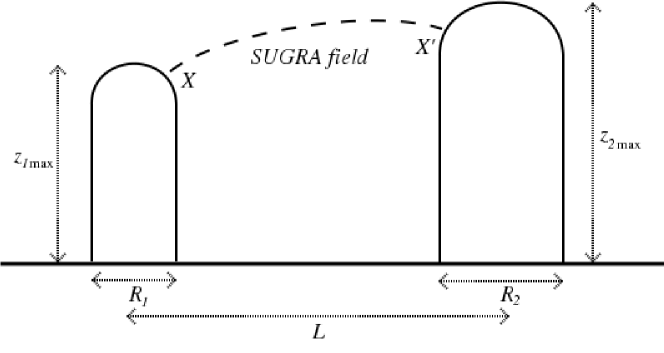
Figure 2: Correlation function of Wilson loops from AdS/CFT. The correlation function is calculated through the exchange of bulk supergravity fields between minimal surfaces attached to each individual Wilson loop. Here $z_{i\,{\rm max}}$ are the depths of the surfaces in the 5th dimension of AdS. The other kinematic notations are as in Fig. 1.

Within the AdS/CFT correspondence, the correlators of Wilson loops in the gauge theory, such as those of Eq. (1), are related to a minimal surface in the bulk of $AdS_{5}$ having as boundaries the two Wilson loops, which corresponds to minimizing the Nambu-Goto action. The analytic solution of a minimal surface problem in Euclidean space (the so-called Plateau problem) is in general a highly nontrivial mathematical issue, and it is even more so in a non flat metric such as $AdS_{5}$. For our purpose, an analytic solution is required in order to adequately perform the Euclidean-to-Minkowskian analytic continuation.

Our guiding line, following Ref. [8], is that the solution simplifies provided the impact parameter distance $L\equiv|\vec{b}|\gg R_{1},R_{2}$. Indeed, when $L\lesssim R_{1},R_{2}$ there exists a connected minimal surface with the sum of the two loops as its disjoint boundary (see $e.g.$ [54]), although its explicit expression is difficult to obtain. However, when $L\gg R_{1},R_{2}$ the minimal surface has two independent, (quasi-)disconnected components: in order to calculate the correlator one then exploits, as in Ref. [55], the explicit solutions corresponding to the two loops connected by the classical supergravity interaction, $i.e.$, by the exchange (see Fig. 2) between them of the lightest fields of the $AdS_{5}$ supergravity, namely the graviton, the anti-symmetric tensor and the dilaton, which are massless, and the tachyonic Kaluza-Klein (KK) scalar mode. This is the case we consider here, using the large-$L$ behavior of the dipole-dipole impact-parameter amplitude evaluated in [8], with a generalization to unequal dipole sizes. As we have already pointed out, we start from the Euclidean formulation of the problem, and so we consider minimal surfaces in $AdS_{5}$ with Euclidean metric in order to obtain the Wilson-loop correlation function in ${\cal N}\!=\!4$ SYM theory in Euclidean space.

Let us recall the main results of [8] and describe briefly how one determines the leading dependence on the impact parameter $L$ and on the rapidity $\chi$ of the various phase shifts (corresponding to the various exchanges of supergravity fields), together with the dependence on the size of the dipoles. For $L\gg R_{1},R_{2}$, and in the weak gravitational field domain, the Euclidean normalized connected correlation function has the form

$${\cal C}_{E} =\exp{\left(\sum_{\psi}\tilde{\delta}_{\psi}\right)}-1\ ,$$ (10)

$$\tilde{\delta}_{\psi} \equiv\frac{1}{4\pi^{2}\alpha^{\prime}{}^{2}}4\int d\tau_{1}d\tau_{2}\,\frac{dz_{1}}{z_{1x}}\frac{dz_{2}}{z_{2x}}\frac{\delta S_{NG}}{\delta\psi}(\tau_{1},z_{1})\ G_{\psi}(X,X^{\prime})\frac{\delta S_{NG}}{\delta\psi}(\tau_{2},z_{2})\ ,$$

where $S_{NG}$ is the Nambu-Goto action, $\alpha^{\prime}=1/\sqrt{4\pi g_{s}N_{c}}$ and $g_{s}$ is the string coupling. Here $\frac{\delta S_{NG}}{\delta\psi}$ is the coupling of the world-sheet minimal surfaces attached to the two Wilson loops to the supergravity field $\psi$. Moreover, $\tau_{i}$ is the proper time on world-sheet $i=(1,2)$, and $z_{1,2}$ are the fifth coordinates of points $X$, $X^{\prime}$ in $AdS_{5}$, namely

$$X=\left(u_{1}^{\mu}\tau_{1}+x_{1}^{\mu}+b^{\mu},z_{1}\right),\quad X^{\prime}=\left(u_{2}^{\mu}\tau_{2}+x_{2}^{\mu},z_{2}\right)\ .$$ (11)

For the relevant four-dimensional vectors we use the notation

$$u_{1}^{\mu} =(1,0,\vec{0}), u_{2}^{\mu}=(\cos\theta,-\sin\theta,\vec{0})\ ,$$ (12)

$$x_{i}^{\mu} =\sigma_{i}(z_{i})\frac{r_{i}^{\mu}}{R_{i}}, \sigma_{i}\in[0,R_{i}],\quad i=1,2\ ,$$

where $\sigma_{i}(z_{i})$ is determined by inverting the solution of the minimal surface equation $z_{i}=z_{i}(\sigma_{i})$. The derivatives $z_{ix}\equiv\frac{\partial z_{i}}{\partial\sigma_{i}}$ are given by [26, 27]

$$z_{ix}=\left(\frac{z_{i{\,\rm max}}}{z_{i}}\right)^{2}\sqrt{1-\left(\frac{z_{i}}{z_{i{\,\rm max}}}\right)^{4}},\quad z_{i\,\rm{max}}={R}_{i}\,\frac{[\Gamma(1/4)]^{2}}{(2\pi)^{3/2}}\ .$$ (13)

In Eq. (10), $G_{\psi}(X,X^{\prime})$ is the Green function relevant to the exchange of field $\psi$, which depends only on invariant bitensors and scalar functions [56] of the AdS invariant

$$u=\frac{(z_{1}-z_{2})^{2}+\sum_{j=1}^{4}(X_{j}-X^{\prime}_{j})^{2}}{2z_{1}z_{2}}\ .$$ (14)

By the change of coordinates $v_{+}=\tau_{2}\sin\theta$, $v_{-}=\tau_{1}-\tau_{2}\cos\theta$, one allows [8] the dependence on $\theta$ to drop from $G_{\psi}(X,X^{\prime})$, so that it can be read off directly from the couplings. One is then able to isolate the leading dependence on $L$ and $R_{i}$ by performing the rescaling $\zeta_{i}=z_{i}/z_{i\,{\rm max}}$, with $\zeta_{i}\in[0,1]$, and $\rho_{\pm}=v_{\pm}/L$: we obtain a factor $L^{2}/z_{1\,{\rm max}}z_{2\,{\rm max}}$ in front of the integrals, and we find the leading term in $u$ to be ${L^{2}}/z_{1\,{\rm max}}z_{2\,{\rm max}}$ times a function of the new integration variables. Working out the Green functions and the couplings corresponding to the exchange of the various supergravity fields, and performing the remaining integrals, it is found that the leading dependence (the “leading” term in $\theta$ is understood as the leading term in $\chi$ after analytic continuation, see below) on $\theta$, $L$ and ${R}_{i}$ for the various terms of (10) is the following:

$$\tilde{\delta}_{S} =\ \ \kappa_{S}\ \frac{1}{\sin\theta}\left(\frac{{R}_{1}{R}_{2}}{L^{2}}\right) \ \ \equiv\ \ a_{S}\ \frac{1}{\sin\theta} \ \ \quad\text{ (KK scalar)}\ ;$$ (15)

$$\tilde{\delta}_{D} =\ \ \kappa_{D}\ \frac{1}{\sin\theta}\left(\frac{{R}_{1}{R}_{2}}{L^{2}}\right)^{3} \ \ \equiv\ \ a_{D}\ \frac{1}{\sin\theta} \ \ \quad\text{ (dilaton)}\ ;$$

$$\tilde{\delta}_{B} =\ \ \kappa_{B}\ \frac{\cos\theta}{\sin\theta}\left(\frac{{R}_{1}{R}_{2}}{L^{2}}\right)^{2} \ \ \equiv\ \ a_{B}\ \frac{\cos\theta}{\sin\theta} \ \ \quad\text{ (antisymmetric tensor)}\ ;$$

$$\tilde{\delta}_{G} =\ \ \kappa_{G}\ \frac{(\cos\theta)^{2}}{\sin\theta}\left(\frac{{R}_{1}{R}_{2}}{L^{2}}\right)^{3} \ \ \equiv\ \ a_{G}\ \frac{(\cos\theta)^{2}}{\sin\theta} \ \ \quad\text{ (graviton)}\ ,$$

factorizing explicitly the angular dependence from the rest. In (15) we keep track of the different dipole sizes. To be complete, the factors $\kappa_{\psi}$ for each supergravity field are given by (see formulas (34,38,49,58) of [8])

$$\kappa_{S}=\frac{g_{s}}{2N_{c}}\frac{10}{\pi^{2}}\ ,\quad\kappa_{D}=\frac{g_{s}}{2N_{c}}\ \frac{3}{16}\left[\frac{\Gamma(1/4)}{2\pi}\right]^{8}\ ,\quad\kappa_{B}={\rm const}\cdot\frac{g_{s}}{2N_{c}}\ ,$$ (16)

where the last constant is yet to be determined, and for the graviton field

$$\kappa_{G}=\frac{g_{s}}{2N_{c}}\frac{15}{2}\left[\frac{\,[\Gamma(1/4)]^{2}}{4\pi}\right]^{4}\ .$$ (17)

The string coupling $g_{s}$ is related to the gauge theory coupling by $g_{\rm YM}^{2}=2\pi g_{s}$. Performing now the analytic continuation $\theta\to-i\chi$, leading to the phase shifts $i\delta_{\psi}\equiv{\tilde{\delta}_{\psi}}(\theta\to-i\chi)$, one finally obtains for the Minkowskian correlation function

$${\cal C}_{M}=\exp\left(i\sum_{\psi}\delta_{\psi}\right)-1\ ,$$ (18)

where $\delta_{\psi}$ are given by

$$\delta_{S}=a_{S}\,\frac{1}{\sinh\chi},\quad\delta_{D}=a_{D}\,\frac{1}{\sinh\chi},\quad\delta_{B}=a_{B}\,\frac{\cosh\chi}{\sinh\chi},\quad\delta_{G}=a_{G}\,\frac{(\cosh\chi)^{2}}{\sinh\chi}\ .$$ (19)

Since the functions $a_{\psi}$ depend only on the combination $\frac{L^{2}}{R_{1}R_{2}}$ of the moduli of the impact parameter and of the dipole sizes $R_{i}$, we will sometimes write ${\cal C}_{M}\equiv{\cal C}_{M}(\chi,L;R_{1},R_{2})$. We notice that under crossing, $i.e.$, under $\chi\to i\pi-\chi$, the phases $\delta_{S}$, $\delta_{D}$ and $\delta_{G}$ are symmetric, while $\delta_{B}$ is antisymmetric. One has then for the definite-signature quantities in (9) the expressions

$${\cal C}_{M}^{(+)} =\cos(\delta_{B})\exp\left[i\left(\delta_{S}+\delta_{D}+\delta_{G}\right)\right]-1\ ,$$ (20)

$${\cal C}_{M}^{(-)} =i\sin(\delta_{B})\exp\left[i\left(\delta_{S}+\delta_{D}+\delta_{G}\right)\right]\ .$$

4 AdS/CFT domain of validity

4.1 The weak field constraint

The range of validity of the calculations above is determined by requiring [8] that the effect of the gravitational perturbation $\delta G_{tt}$ generated by each of the string world-sheets on the other one is smaller than the background metric $G_{tt}$, therefore ensuring that one is actually working in the weak-field limit. Considering the effect of world-sheet 2 on world-sheet 1 (see Fig. 2) the strongest constraint is obtained from the evaluation of the maximal gravitational field produced at the point $\tau_{1}=0,$ where the distance between the loops is minimal. The weak gravitational field requirement reads

$$\frac{\delta G_{tt}}{G_{tt}}\ll 1,\quad G_{tt}\equiv\frac{1}{z_{1}^{2}}\ ,$$ (21)

where $G_{tt}$ is the background metric term coming from the $AdS_{5}$ Fefferman-Graham parameterization. In order to find the explicit expression of condition (21), we note that the phase shift in (10) can be also interpreted as an integral over the string world-sheet 1 (at $\theta=0$) of the corresponding supergravity field $\psi(X^{\prime})$ produced by the other, tilted world-sheet 2 (at $\theta$), namely

$$\delta\psi(X(\tau_{1},z_{1}))=\frac{1}{2\pi\alpha^{\prime}}\int 2d\tau_{2}\frac{dz_{2}}{z_{2_{x}}}\ G_{\psi}(X,X^{\prime})\ \frac{\delta S_{NG}}{\delta\psi}(\tau_{2},z_{2})\ .$$ (22)

Applying this generic equation to the specific dominant graviton contribution, one writes the graviton coupling by expanding the Nambu-Goto action, namely

$$\sqrt{h}\left[\frac{\delta h_{\tau\tau}}{2h_{\tau\tau}}+\frac{\delta h_{\sigma\sigma}}{2h_{\sigma\sigma}}\right]\sim\frac{z_{2\,{\rm max}}^{2}}{2{z_{2}}^{2}}\,\delta h_{\tau\tau}\sim(\cos\theta)^{2}\,\delta G_{tt}\ ,$$ (23)

where $h_{ab}$ is the induced metric on world-sheet 1, and we have retained only the dominant part of the field after analytic continuation $\theta\to-i\chi$. The field produced at the point $\tau_{1}=0$ by the second (tilted) world-sheet is then given by

$$\frac{1}{2\pi\alpha^{\prime}}\int 2d\tau_{2}\frac{dz_{2}}{z_{2x}}\frac{z_{2\,{\rm max}}^{2}}{2z_{2}^{2}}\left\langle{\delta h_{\tau\tau}^{\theta}\delta h_{\tau\tau}^{\theta=0}}\right\rangle\ ,$$ (24)

where the correlation function

$$\left\langle{\delta h_{\tau\tau}^{\theta}\delta h_{\tau\tau}^{\theta=0}}\right\rangle=\frac{1}{z_{1}^{2}z_{2}^{2}}\left[2G(u)(\cos\theta)^{2}+H(u)\right]\$$ (25)

is given [57] in terms of the functions $G(u)\sim(3/32\pi^{2})\cdot 1/u^{4}$ and $H(u)\sim(-1/48\pi^{2})\cdot 1/u^{2}$ for large $u,$ where $u$ is the AdS invariant (14). Using $u(\tau_{1}=0)\sim(L^{2}+\tau_{2}^{2})/(2z_{1}z_{2})$ one gets

$$\delta G_{tt}\propto(\cos\theta)^{2}\,\int\frac{dz_{2}}{z_{2x}}\frac{z_{2\,{\rm max}}^{2}}{z_{2}^{2}}\frac{1}{z_{1}^{2}z_{2}^{2}}\int_{-\infty}^{\infty}d\tau_{2}\,\frac{z_{1}^{4}z_{2}^{4}}{(L^{2}+\tau_{2}^{2})^{4}}\ ;$$ (26)

one then performs the rescaling $\tau_{2}\to\tau_{2}/L,$ $z_{2}\to z_{2}/z_{2\,{\rm max}},$ with $z_{2\,{\rm max}}\propto R_{2}$, and finds the constraint

$$\frac{\delta G_{tt}}{G_{tt}}\propto\frac{z_{1}^{4}R_{2}^{3}}{L^{7}}(\cos\theta)^{2}\ll 1\ .$$ (27)

This constraint is most restrictive when evaluated at $z_{1}=z_{1\,{\rm max}}\propto R_{1}$, which is as far as the string world-sheet extends into the $5$th dimension of $AdS_{5},$ see Fig. 2. Performing the analytic continuation $\theta\to-i\chi$, and interchanging the rôles of the two world-sheets by switching the subscripts 1 and 2 in the results above in order to get the maximal constraint, one finally obtains

$$\left(\frac{L^{2}}{{R}_{1}{R}_{2}}\right)^{\frac{7}{2}}{\rm min}\left(\sqrt{\frac{{R}_{1}}{{R}_{2}}},\sqrt{\frac{{R}_{2}}{{R}_{1}}}\,\right)\gg\ \varsigma^{2}\quad\!\Rightarrow\quad\!{L^{2}}\gg L_{max}^{2}\equiv\frac{{{R}_{1}{R}_{2}}\varsigma^{\frac{4}{7}}}{\left[{\rm min}\left(\sqrt{\frac{{R}_{1}}{{R}_{2}}},\sqrt{\frac{{R}_{2}}{{R}_{1}}}\,\right)\right]^{\frac{2}{7}}}\ ,$$ (28)

and in this region the phase $\delta_{G}$ is actually small, as it should be. It is interesting to remark that the smaller the dipole size, the larger the impact-parameter region where the weak field approximation is valid, as we may expect from physical intuition. Moreover, considering the possibility of an energy-dependent dipole size inside a target, $e.g.$ due to high density effects, the size dependence may even strengthen the cross section bound (see next section 4.2) through a weaker energy dependence of the impact-parameter limit $L_{max}$. Let us for instance assume an energy dependence $R_{1}^{2}\sim R_{2}^{2}\varsigma^{-\lambda}$ of the smaller dipole size: in this case one would find a weaker constraint on $L$,

$$\left(\frac{L}{R_{2}}\right)^{2}\gg\ \varsigma^{\frac{4}{7}-\frac{3}{7}\lambda}\ .$$ (29)

4.2 The elastic eikonal hypothesis

From expression (1) one can determine the impact-parameter partial amplitude $a(\chi,\vec{b})$ corresponding to the dipole-dipole elastic amplitude ${\cal A}$, $i.e.$ (suppressing the sizes of the dipoles) $a(\chi,\vec{b})=-i{\cal C}_{M}(\chi,\vec{b})$. In the large-$L$ region, following section 3, the AdS/CFT contribution reads

$$a_{tail}(\chi,\vec{b})=i\left[1-\exp\left(i\sum_{\psi}\delta_{\psi}\right)\right]\ ,$$ (30)

with the phase shifts specified by (19). This expression can be trusted as long as the solution for the minimal surface problem is disconnected, and above all, as remarked in the preceding subsection, as long as the weak gravitational field constraint (28) is satisfied. Note that since expression (30) verifies the relation

$${\rm Im}\ a_{tail}(\chi,\vec{b})=\frac{1}{2}\left|a_{tail}(\chi,\vec{b})\right|^{2}\ ,$$ (31)

it corresponds to a purely elastic amplitude, in agreement with the planar limit implied by the AdS/CFT correspondence.

The result (28) calls for an important comment: it expresses a stringent constraint on the impact-parameter range due to the weak gravitational field condition required in applying the AdS/CFT correspondence. Let us now add to the discussion a possible extension of the results, obtained adopting the $S$-matrix point-of-view, but not a priori borne out by the dual AdS/CFT picture.

From the $S$-matrix point-of-view, the exponential form of (30) (see also (18)) is typical of a resummation of non-interacting ($i.e.$, independent) colorless exchanges (on the gauge theory side) which can be taken into account in order to possibly enlarge the domain of validity of (30). This amounts to assume the validity of the eikonal approximation for a purely elastic scattering amplitude (see [59, 60, 61] for the eikonal approximation in QED; for QCD see $e.g.$ [62]). However, in the framework of the microscopic theory, $i.e.$, the 4-dimensional gauge theory at strong coupling, there is no rigorous theoretical derivation of the eikonal formula. In fact, as a result of our previous analysis, we do not expect this independent resummation to be valid from the AdS/CFT correspondence point-of-view, since a strong gravitational field in the bulk near the relevant minimal surfaces is expected to be the seed of graviton self-interactions, which would spoil the independent emission of the gravitational eikonal formalism.

Yet, for completion, let us suppose that the eikonal formalism for the elastic amplitude may be extended in some larger phase-space region and thus examine, from the empirical $S$-matrix point-of-view, whether and down to which value of the impact-parameter separation the formula (30) could be used beyond the constraint (28). As a first step beyond our AdS/CFT correspondence result, one could infer from an $S$-matrix model formulation that the amplitude (30) is reliable as long as the dominant graviton-induced phase shift $\delta_{G}$ is small. Following formulas (19), this means that $\frac{L^{2}}{{R}_{1}{R}_{2}}\gg\left(\kappa_{G}\frac{(\cosh\chi)^{2}}{\sinh\chi}\right)^{\frac{1}{3}}\sim\left(\kappa_{G}\varsigma\right)^{\frac{1}{3}}.$ In fact the minimal impact-parameter value for the eikonal formula (30) to be physically sensible from the 4-dimensional point-of-view is more precisely

$${L^{2}}>L^{2}_{min}\equiv{{R}_{1}{R}_{2}}\left(\frac{\kappa_{G}}{\pi}\ \varsigma\right)^{\frac{1}{3}}$$ (32)

requiring the phase shift $\delta_{G}\leq\pi,$ see Eq. (19). This extreme minimal bound ensures that ${\rm Im}\,a_{tail}(\chi,\vec{b})$ be not oscillating with $L$: since it is just proportional, $via$ the optical theorem, to the $L$-dependent partial cross section, a non-oscillating behavior is expected. Indeed, it is reasonable to expect that more and more inelastic channels would open up when going from the peripheral to the central impact-parameter domain.

From the dual gravitational point-of-view, the problem seems severe. Studies of the gravitational eikonal approximation already exist in the literature [12, 16, 17, 18, 19, 20, 24]; however, the precise question which is relevant in our case is beyond which value in the large impact-parameter range the eikonal expression (30) for a purely elastic amplitude is expected to be valid. This is equivalent to ask up to what impact-parameter distance it is mainly the exchange of independent gravitons in the bulk which builds the whole amplitude. Using our minimal surface approach, we see that the limitation to a weak field approximation for the gravitational field at the tip of the minimal surfaces gives a stronger constraint than the one (32) coming from the $S$-matrix model point-of-view.

4.3 Characteristic impact-parameter scales

Let us consider a range of validity of (30) varying from its AdS/CFT value defined by (28) to its maximal $S$-matrix model extension (32). We are lead to define a characteristic distance $L_{tail}$ such that for $L=|\vec{b}|>L_{tail}(s)$ the impact-parameter scattering amplitude is given by Eq. (30). One can then divide the whole impact-parameter space into a $tail$ region ($L>L_{tail}$), and a $core$ region ($L<L_{tail}$) where inelastic channels are supposed to open up. More specifically, the following regions are identified.

1. At large distances $L>L_{max},$ whose exact expression is given by (28), the gravitational field in the bulk is weak enough, and the contribution of the disconnected minimal surface gives a rigorous holographic determination of the impact-parameter tail of the scattering amplitude.

2. At moderately large distances $L_{min}<L<L_{max}$, where $L_{min}$ has been defined in (32), the strong gravitational field is expected to generate a non zero ${\rm Im}\,\delta_{G}$ leading to inelastic contributions on the gauge theory side, and hence to ${\rm Im}\ a_{tail}(\chi,\vec{b})>\frac{1}{2}|a_{tail}(\chi,\vec{b})|^{2}$ contrary to (31). The minimal surface is still disconnected but the gravitational field begins to become strong in some relevant region in the bulk. Nevertheless, for the sake of completeness, we will investigate what happens assuming the validity of the elastic eikonal expression up to $L_{tail}$, lying somewhere in the range $L_{min}\leq L_{tail}\leq L_{max}$.

3. For $L_{connect}<L<L_{min}$ the elastic eikonal expression (30) is no more reliable, even from the $S$-matrix point-of-view. An eikonal formula may still be valid with an imaginary contribution to the phase shifts but it cannot be obtained through the weak gravity regime of the AdS/CFT correspondence, even if the minimal surface is still made of disconnected surfaces joined by interacting fields.

4. Finally, for even smaller distances $L\leq L_{connect}$ the Gross-Ooguri transition takes place, and the minimal surface solution becomes connected. In this region, the AdS/CFT description goes beyond the interaction mediated by supergravity fields.

Region 1 and possibly part of region 2 constitute the impact-parameter tail region, while the regions 3 and 4 constitute the central impact-parameter core region. To incorporate these regions in our analysis we need to use information coming from a source other than the AdS/CFT correspondence: in practice, we will use the unitarity constraint

$${\rm Im}\ a(\chi,\vec{b})\leq 2\ .$$ (33)

Since we know precisely $a(\chi,\vec{b})$ only in the $tail$ region, we are able to determine only part of the full scattering amplitude, $i.e.$, the large impact-parameter contribution ${\cal A}_{tail}$,

$${\cal A}\equiv{\cal A}_{core}+{\cal A}_{tail}\ ;\quad{\cal A}_{tail}(s,t;\vec{R}_{1},\vec{R}_{2})=2is\int_{L\geq L_{tail}}d^{2}\vec{b}\ e^{i\vec{q}\cdot\vec{b}}\,\left[1-e^{\left(i\sum_{\psi}\delta_{\psi}\right)}\right]\ ,$$ (34)

where ${\cal A}_{core}$ will be constrained by the unitarity bound (33). Exploiting this expression and (33), we will be able to set a lower and an upper bound on the large-$s$ behavior of the full amplitude depending on the $s$-dependence of $L_{tail}$.

An important addendum to this discussion is related to its modification due to energy-dependent dipole sizes, as in (29). Indeed, sticking to the rigorous result coming from the AdS/CFT correspondence in the case of a dipole of given size $R$ scattering on a dipole of energy-dependent size $R(\varsigma)\sim R\varsigma^{-\frac{\lambda}{2}},$ one finds $L_{tail}\sim R\varsigma^{\frac{2}{7}-\lambda\frac{3}{14}}.$ This has the expected effect of enlarging the domain of elasticity and, as we shall see now, to strengthen the high-energy bound on the total cross section.

4.4 A convergence problem for ${\rm Re}\,{\cal A}_{tail}$

As a preliminary, we have to discuss the convergence properties of ${\cal A}_{tail}$ in (34). Performing the angular integration, one has (with $q\equiv|\vec{q}\,|$)

$${\cal A}_{tail}(s,t;\vec{R}_{1},\vec{R}_{2})=-4\pi is\int_{L_{tail}}^{\infty}dL\,L\,J_{0}(qL)\,{\cal C}_{M}(\chi,L;R_{1},R_{2})\ .$$ (35)

Following expression (19), at large $L$ the integrand is dominated by the tachyonic KK scalar exchange and behaves as

$$L\sqrt{\frac{2}{\pi qL}}\cos\left(qL-\frac{\pi}{4}\right)\left[i\left(\kappa_{S}\frac{R_{1}R_{2}}{L^{2}}\frac{1}{\sinh\chi}\right)-\frac{1}{2}\left(\kappa_{S}\frac{R_{1}R_{2}}{L^{2}}\frac{1}{\sinh\chi}\right)^{2}\right],$$ (36)

and since the imaginary part is bounded by $L^{-3/2}$, while the real part is bounded by $L^{-7/2}$, the integral is convergent as long as $q\neq 0$.

However, if one sets $q=0$ directly in the integrand, since $J_{0}(0)=1$ one finds a logarithmic divergence in the real part of the amplitude, coming from this KK scalar contribution. One can easily isolate the divergent part by writing

$${\cal A}_{tail}(s,t;\vec{R}_{1},\vec{R}_{2})= -4\pi is\int_{L_{tail}}^{\infty}dL\,L\,J_{0}(qL)\,\times$$ (37)

$$\times\left[\frac{R_{1}R_{2}}{L^{2}}\frac{i\kappa_{S}}{\sinh\chi}+\left({\cal C}_{M}(\chi,L;R_{1},R_{2})-\frac{R_{1}R_{2}}{L^{2}}\frac{i\kappa_{S}}{\sinh\chi}\right)\right]\,.$$

The term in brackets is convergent at $q=0$; to treat the other term one divides the integral as follows:

$${\cal A}_{tail}^{div}(s,t;\vec{R}_{1},\vec{R}_{2})\equiv -4\pi is\int_{L_{tail}}^{\infty}dL\,L\,J_{0}(qL)\,\frac{R_{1}R_{2}}{L^{2}}\frac{i\kappa_{S}}{\sinh\chi}$$ (38)

$$\,= \,4\pi\kappa_{S}\frac{s}{\sinh\chi}R_{1}R_{2}\left[\int_{1}^{\infty}\frac{d\lambda}{\lambda}\,J_{0}(\lambda)+\int_{qL_{tail}}^{1}\frac{d\lambda}{\lambda}\,(J_{0}(\lambda)-1)\,+\right.$$

$$\left.\hphantom{4\pi\kappa_{S}\frac{s}{\sinh\chi}R_{1}R_{2}\bigg{[}}+\int_{qL_{tail}}^{1}\frac{d\lambda}{\lambda}\right].$$

It is now easy to see that the only divergent term when $q\to 0$ is the last one, and so we conclude

$${\cal A}_{tail}^{div}(s,t\to 0;\vec{R}_{1},\vec{R}_{2})=4\pi\kappa_{S}\frac{s}{\sinh\chi}R_{1}R_{2}\log\frac{1}{qL_{tail}}+{\rm finite\,\,terms}\ ;$$ (39)

recalling the relation (4) between $\chi$ and $s$ one then obtains in the high-energy limit

$${\cal A}_{tail}^{div}(s,t\to 0;\vec{R}_{1},\vec{R}_{2})=8\pi\kappa_{S}m_{1}m_{2}R_{1}R_{2}\log\frac{1}{qL_{tail}}+{\rm finite\,\,terms}\ .$$ (40)

In fact, one should distinguish the mathematical problem of determining the real part of the amplitude from a deeper physical one concerning the AdS/CFT correspondence itself. Indeed, since the imaginary part of the amplitude is always finite in the $t\to 0$ limit, and moreover, as we will see in a moment, also analytic in $s$, it is known how to obtain the real part by means of a dispersion relation, which yields a finite result. However, on the gravity side, it is as yet unclear what is the origin of this divergence, that we expect to be cancelled by effects which do not show up at the given level of supergravity approximation of the AdS/CFT correspondence. Moreover, for our purpose, the dependence on the energy is weak, coming through the dependence of $L_{tail}$ on $s$. In the following we will then discard this divergence, focusing on the dominant contribution at large $s$; conceptually, it may be a relevant issue, but we delay this study for the future.

5 The ${\cal N}=4$ SYM forward amplitude

5.1 Total cross section

We start from the imaginary part of the amplitude at $t=0$, which is related to the dipole-dipole elastic total cross section by means of the optical theorem. The contribution $\sigma_{tail}$ to the total cross section of the large impact-parameter region as obtained from AdS/CFT is given by

$$\sigma_{tail} {\mathop{\simeq}_{s\to\infty}}\frac{{\rm Im}\,{\cal A}_{tail}(s,0;\vec{R}_{1},\vec{R}_{2})}{s}=-4\pi\int_{L_{tail}}^{\infty}\!\!dL\,L\ {\rm Re}\,{\cal C}_{M}(\chi,L;R_{1},R_{2})$$ (41)

$$=4\pi\int_{L_{tail}}^{\infty}\!\!dL\,L\,\left[1-\cos\left(\sum_{\psi}\delta_{\psi}\right)\right].$$

The $\chi$-dependence at large energy induces a hierarchy between the different contributions. This hierarchy is clearly revealed after performing the change of variables

$$L\to\lambda\equiv(\sinh\chi)^{-\frac{1}{6}}\frac{L}{\sqrt{R_{1}R_{2}}};\quad L_{tail}\to\lambda_{tail}=(\sinh\chi)^{-\frac{1}{6}}\frac{L_{tail}}{\sqrt{R_{1}R_{2}}}\ ,$$ (42)

which yields (rescaling with $\sinh\chi$ instead of $\cosh\chi$ allows to keep manifest the symmetry under crossing, $i.e.$, under $\chi\to i\pi-\chi$, of the various phase shifts in formulas (19))

$$\sigma_{tail}= 4\pi(\sinh\chi)^{\frac{1}{3}}R_{1}R_{2}\int_{\lambda_{tail}}^{\infty}\!d\lambda\,\lambda\,\Bigg{[}1-\cos\Bigg{(}\frac{\kappa_{S}}{\lambda^{2}}\frac{1}{(\sinh\chi)^{\frac{4}{3}}}+\frac{\kappa_{D}}{\lambda^{6}}\frac{1}{(\sinh\chi)^{2}}\,+$$ (43)

$$\hphantom{4\pi(\sinh\chi)^{\frac{1}{3}}R_{1}R_{2}\int_{\lambda_{tail}}^{\infty}\!d\lambda\,\lambda\,\Bigg{[}}+\frac{\kappa_{B}}{\lambda^{4}}\frac{\coth\chi}{(\sinh\chi)^{\frac{2}{3}}}+\frac{\kappa_{G}}{\lambda^{6}}(\coth\chi)^{2}\Bigg{)}\Bigg{]}\,.$$

The integral is clearly finite:

• the quantity in braces is always bounded between 0 and 2, which indeed corresponds to the unitarity constraint on the impact-parameter amplitude,

• in the large $\lambda$ limit the integrand behaves as $\lambda^{-3}$ (corresponding to the KK scalar contribution to ${\rm Im}\,{\cal A}_{tail}(s,0)$).

The overall convergence is then ensured, contrary to the case of the real part. Note that the leading term (the last one in (43)) is crossing-symmetric, thus corresponding to “Pomeron exchange” in the $S$-matrix language, while the first subleading term, coming from antisymmetric-tensor exchange (the before-last one in (43)), is crossing-antisymmetric under $\chi\to i\pi-\chi$, thus corresponding to “Odderon exchange”. At large energy the dominant contribution is the one from graviton exchange. Indeed, recalling the relation (4) between $\chi$ and $s$ we obtain for $s\to\infty$

$$\sigma_{tail} \mathop{\simeq}_{s\to\infty}4\pi{R}_{1}{R}_{2}\varsigma^{\frac{1}{3}}\int_{\lambda_{tail}}^{\infty}d\lambda\,\lambda\left[1-\cos\left(\frac{\kappa_{G}}{\lambda^{6}}\right)\right]$$ (44)

$$\mathop{=}_{\phantom{s\to\infty}}\frac{2\pi}{3}{R}_{1}{R}_{2}\,\varsigma^{\frac{1}{3}}\int_{0}^{\mu_{tail}}d\mu\,\mu^{-\frac{4}{3}}\left[1-\cos\left(\kappa_{G}\mu\right)\right]$$

$$\mathop{=}_{\phantom{s\to\infty}}\frac{2\pi}{3}{R}_{1}{R}_{2}\,\left(\frac{\varsigma}{\mu_{tail}}\right)^{\frac{1}{3}}\int_{0}^{1}dx\,x^{-\frac{4}{3}}\left[1-\cos\left(\kappa_{G}\mu_{tail}x\right)\right]\ ,$$

where we have set

$$\mu\equiv\lambda^{-{6}}\ ;\quad\mu_{tail}=\lambda^{-{6}}_{tail}\ ;\quad x=\frac{\mu}{\mu_{tail}}\ .$$

To complete the calculation of the high-energy behavior of $\sigma_{tail}$ we need to know the limit of validity of the application of AdS/CFT and thus how $L_{tail}$ depends on $s$. Let us consider the parameterization

$$L_{tail}=\lambda_{0}\sqrt{R_{1}R_{2}}\ \varsigma^{\beta}\Rightarrow\lambda_{tail}=\lambda_{0}\ \varsigma^{\beta-\frac{1}{6}}\ ;\quad\quad\mu_{tail}=\lambda_{0}^{-6}\varsigma^{1-6\beta}\ ,$$ (45)

where $\lambda_{0}$ may have some residual dependence on $R_{1,2}$ (see $e.g.$ (28)). If $\beta<\frac{1}{6}$ then $\lambda_{tail}\to 0$ and $\mu_{tail}\to\infty$ as the energy increases, and so $\sigma_{tail}\sim\varsigma^{\frac{1}{3}}$; if $\beta>\frac{1}{6}$ then $\mu_{tail}\to 0$ and $\lambda_{tail}\to\infty$, and so $\sigma_{tail}\sim\varsigma^{\frac{1}{3}}\varsigma^{\frac{5}{3}(1-6\beta)}=\varsigma^{2-10\beta}$. Finally, for $\beta=\frac{1}{6}$ a constant $\lambda_{tail}$ is found, and the integral cannot modify the $s$-dependence. Summarizing, we have for large $s$

$$\sigma_{tail} \mathop{\simeq}_{\phantom{s\to\infty}}\ \frac{2\pi}{3}\lambda_{0}^{2}R_{1}R_{2}\varsigma^{2\beta}\int_{0}^{1}dx\,x^{-\frac{4}{3}}\left[1-\cos\left(\kappa_{G}\lambda^{-6}_{0}\varsigma^{1-6\beta}x\right)\right]$$ (46)

$$\mathop{\sim}_{s\to\infty}\frac{2\pi}{3}R_{1}R_{2}\ \left\{\begin{aligned} &\varsigma^{\frac{1}{3}}\frac{3\pi\kappa_{G}^{\frac{1}{3}}}{\Gamma(1/3)}&&\beta<\frac{1}{6}\ ,\\ &\varsigma^{\frac{1}{3}}\lambda_{0}^{2}\int_{0}^{1}dx\,x^{-\frac{4}{3}}\left[1-\cos\left(\kappa_{G}\lambda_{0}^{-6}x\right)\right]&&\beta=\frac{1}{6}\ ,\\ &\varsigma^{2-10\beta}\frac{1}{2}\kappa_{G}^{2}\lambda_{0}^{-10}&&\beta>\frac{1}{6}\ .\end{aligned}\right.$$

We are now in the position to determine a lower and an upper bound on the high-energy behavior of the dipole-dipole total cross section. Since obviously $\sigma_{tot}>\sigma_{tail}$, Eq. (46) provides a lower bound. The overall unitarity constraint Eq. (33) allows one to put an upper bound on the contribution from the $core$ region $L<L_{tail}$, $i.e.$, $\sigma_{core}\leq 4\pi L_{tail}^{2}=4\pi\lambda_{0}^{2}R_{1}R_{2}\varsigma^{2\beta}$, and thus on the whole total cross section,

$$\sigma_{tot}=\sigma_{core}\!+\sigma_{tail}<4\pi\lambda_{0}^{2}R_{1}R_{2}\varsigma^{2\beta}\left\{1+\frac{1}{6}\int_{0}^{1}dx\,x^{-\frac{4}{3}}\left[1-\cos\left(\kappa_{G}\lambda^{-6}_{0}\varsigma^{1-6\beta}x\right)\right]\right\}\!\,.$$ (47)

We have included here only the leading part of the $tail$ contribution at high energy. A more rigorous way to write the $\beta$-dependent bounds on the high-energy behavior of $\sigma_{tot}$ is the following,

$$\min\left(\frac{1}{3},2-10\beta\right)\leq\lim_{\varsigma\to\infty}\frac{\log\sigma_{tot}}{\log\varsigma}\leq\max\left(\frac{1}{3},2\beta\right),$$ (48)

which in particular, using the value $\beta=\frac{2}{7}$ coming from the weak field constraint (28), yields the rigorous bound

$$-\frac{6}{7}\leq\lim_{\varsigma\to\infty}\frac{\log\sigma_{tot}}{\log\varsigma}\leq\frac{4}{7}\,.$$ (49)

The following remarks are in order.

1. For $\beta<\frac{1}{6}$, at sufficiently high energy one would have $L_{tail}<L_{min}$, thus entering the unphysical region where the impact-parameter partial amplitude is infinitely oscillating between 0 and 1. In this case the total cross section would become purely elastic at high energy, while one expects the opening of more and more inelastic channels as the energy increases: this means that one lies beyond the applicability of the elastic eikonal approximation.

2. At $\beta=\frac{1}{6},$ corresponding to $L_{tail}/L_{min}=const.$, the $tail$ and $core$ contributions have the same high-energy behavior. In this case $\lambda_{tail}$ (or, equivalently, $\mu_{tail}$) does not depend on energy. However, one has to verify the non-oscillating behavior condition

   $$\lambda_{tail}\geq\left(\frac{\kappa_{G}}{\pi}\right)^{\frac{1}{6}},\quad\quad\mu_{tail}\leq\frac{\pi}{\kappa_{G}}\ .$$ (50)

3. For $\frac{1}{6}<\beta\leq\frac{2}{7}$, which corresponds to $L_{min}<L_{tail}<L_{max}$ (strictly speaking, at sufficiently high energy), the $core$ region dominates, while the $tail$ region gives a subleading contribution as $s\to\infty$. The two bounds determine a window of possible power-law behaviors.

4. For the maximal value $\beta=\frac{2}{7}$, $i.e.$, for $L_{tail}/L_{max}=const.$, the total cross section behavior is constrained to be such that $\sigma_{tot}\leq{const.}\times\varsigma^{\frac{4}{7}}.$ This maximal value is determined from the requirement that the AdS/CFT correspondence can be reliably applied, $i.e.$, that the constraint (32) for the gravitational perturbation to be weak is verified. In fact, this is the rigorous result obtained by means of the AdS/CFT correspondence, since for smaller $\beta$ one expects inelastic contributions coming from a strong dual gravitational field.

5. One could also consider $\beta>\frac{2}{7}$, but in that case one would only obtain a weaker bound on the total cross section. Indeed, in doing so one would overestimate the contribution of the $core$, including in it the impact-parameter region $L_{max}<L<L_{tail}$, where the amplitude is reliably described by the eikonal AdS/CFT expression.

In the rest of this paper we will thus consider the $\beta$-dependence in the domain $\frac{1}{6}\leq\beta\leq\frac{2}{7}$. The limiting values have the following characteristics: $\beta=\frac{1}{6}$ is the minimal admissible value for which the eikonal approximation using real phase shifts could be valid, and $\frac{2}{7}$ is the absolute bound coming from the AdS/CFT correspondence. Note that from Eq. (46) we see that ${\rm Im}\,{\cal A}_{tail}(s,0)=\varsigma^{1+\gamma}\times(s\text{-independent})$ is analytic in $s$, with a branch point at $s=0$.

Figure 3: Upper and lower bounds on the high-energy behavior of total cross sections. The bounds on the total cross section exponent $\gamma$, $i.e.$, on the Pomeron intercept minus one, are displayed as a function of the power law exponent $\beta$ of $L_{tail}\propto\varsigma^{\beta}$. Solid line: upper bound, coming from the $core$ contribution for $\frac{1}{6}\leq\beta\leq\frac{2}{7}$. Long-dashed line: lower bound, coming from the $tail$ contribution for $\beta>\frac{1}{6}$. Short-dashed line: weaker upper bound for $\beta>\frac{2}{7}$, obtained by overestimating the $core$ contribution (see text). We singularize the value $\beta=\frac{1}{5}$ below which the $tail$ contribution and thus the total cross section are bounded to grow.

5.2 Asymptotic forward phase

A general result regarding scattering amplitudes at high-energy relates the phase $\varphi$ of the amplitude to the leading behavior in $s$ (see $e.g.$ [63, 64] and references therein): for a symmetric amplitude behaving as $\sim s^{\alpha}$ at high energy one has ${\cal A}^{(+)}\sim\pm s^{\alpha}e^{i\pi(1-\frac{\alpha}{2})}$, while for an antisymmetric amplitude with the same leading $s$-dependence one finds ${\cal A}^{(-)}\sim\pm s^{\alpha}e^{i\pi(\frac{1}{2}-\frac{\alpha}{2})}$. Note that for the dominant contribution the sign ambiguity is fixed by asking for a positive total cross section. This result is a consequence of analyticity, and it is obtained through the application of the Phragmén-Lindelöf theorem to the function ${\cal A}^{(\pm)}/(s-u)^{\alpha}$ ($u$ is here the usual Mandelstam variable). Hence we have at asymptotic energy

$$\frac{{\rm Im}\,{\cal A}^{(+)}}{{\rm Re}\,{\cal A}^{(+)}}=-\tan\frac{\pi\alpha}{2}\ ;\quad\quad\frac{{\rm Im}\,{\cal A}^{(-)}}{{\rm Re}\,{\cal A}^{(-)}}=\cot\frac{\pi\alpha}{2}\ .$$ (51)

Although this result holds in general for any value of $t$ along the “Regge trajectory” $\alpha(t)$, we consider here the forward amplitude. Using (51) for a positive signature amplitude ${\cal A}^{(+)}$ with $\alpha=1+\gamma$, and taking $\gamma=\gamma(\beta)$ to be the upper bound on the exponent determined above in section 5.1, we find that at large $s$

$${\cal A}^{(+)}=C\varsigma^{1+\gamma}e^{i\frac{\pi}{2}(1-\gamma)},\quad\gamma(\beta)=\max\left(\frac{1}{3},2\beta\right)\ ,$$ (52)

where the phase $\varphi=\frac{\pi}{2}(1-\gamma)$ varies in the range between $\varphi=\frac{3\pi}{14}$, for the maximally $core$-dominated $\beta=\frac{2}{7}$ amplitude, and $\varphi=\frac{\pi}{3}$ for the $tail$-dominated result at $\beta\leq\frac{1}{6}$. Here $C$ is a positive constant, and we fix the sign ambiguity of the amplitude by requiring the positivity of the total cross section.

The interesting outcome of these analyticity properties is that we gain a new constraint on the overall amplitude, which can help complementing the knowledge of the $tail$ region from AdS/CFT. As an example, one may consider a “black disk model” [65], where one assumes the eikonal approximation in the whole $tail$ ($i.e.$, $\beta=\frac{1}{6}$), and a maximally inelastic (“black disk”) amplitude in the $core$ ($i.e.$, $a(\chi,\vec{b})\sim i$). One then obtains the frontier between $tail$ and $core$ being fixed at $\kappa_{G}\mu_{tail}\sim\frac{\pi}{2}$ with a forward amplitude consistent with analyticity and unitarity and satisfying the constraint relation (50).

5.3 Subleading contributions

The expression Eq. (43) shows clearly the hierarchy in energy of the contributions of the various supergravity fields. Indeed, at large $s$, keeping only the leading contribution from each field, we have for the subleading part of the total cross section

$$\sigma^{subleading}_{tail}\simeq 4\pi\varsigma^{\frac{1}{3}}R_{1}R_{2}\int_{\lambda_{tail}}^{\infty}d\lambda\,\lambda\,\sin\left(\frac{\kappa_{G}}{\lambda^{6}}\right)\left(\frac{\kappa_{S}}{\lambda^{2}}\frac{1}{\varsigma^{\frac{4}{3}}}+\frac{\kappa_{D}}{\lambda^{6}}\frac{1}{\varsigma^{2}}+\frac{\kappa_{B}}{\lambda^{4}}\frac{1}{\varsigma^{\frac{2}{3}}}\right)\ .$$ (53)

The well-known “absorption” phenomenon appears in (53), since the secondary contributions are shielded by the $\sin\left(\frac{\kappa_{G}}{\lambda^{6}}\right)$ coming from the leading graviton contribution. Its natural interpretation in a $S$-matrix framework comes from the initial and final state elastic interactions which correct the “bare” secondary contributions.

For $\beta>\frac{1}{6}$, in which case $\lambda^{-1}_{tail}\to 0$ in (53), we have for the $tail$ contributions

$$\begin{aligned} &\text{graviton \phantom{({\it tail}\ \rm{and}\ {\it core}\/)}}&&\longrightarrow&&2-10\beta\\ &\text{antisymmetric tensor}&&\longrightarrow&&1-8\beta\\ &\text{KK scalar}&&\longrightarrow&&\phantom{1}-6\beta\\ &\text{dilaton}&&\longrightarrow&&\phantom{1}-10\beta\ .\end{aligned}$$ (54)

The secondary contributions in the $$core \beta=\frac{1}{6} \lambda_{tail}\sim const. s tail$$ are neither determined nor usefully constrained by unitarity. Note that, in the limiting case , with , the leading -dependence of the various contributions to the total cross section obey the following hierarchy:

$$\begin{aligned} &\text{graviton ({\it tail}\ \rm{and}\ {\it core}\/)}&&\longrightarrow&&\textstyle\frac{1}{3}\\ &\text{antisymmetric tensor}&&\longrightarrow&-&\textstyle\frac{1}{3}\\ &\text{KK scalar}&&\longrightarrow&-&1\phantom{\frac{1}{1}}\\ &\text{dilaton}&&\longrightarrow&-&\textstyle\frac{5}{3}\ .\end{aligned}$$ (55)

Starting from the graviton, the intercept of the other contributions is obtained subtracting $2/3$ each time. Note that, when expanding the eikonal expression, one must be aware that subleading contributions from a field with a larger intercept mix with the leading contributions of the less relevant fields.

In the “black disk model” [65], one assumes total absorption in the $core$ region, an thus formula (53) would give the whole contribution to the total cross section from subleading contributions. Hence, in that case one would determine the effective hierarchy of intercepts to be given by (LABEL:Hier) with $\beta=\frac{1}{6}$. In particular, the “Odderon” contribution, $via$ Gauge/Gravity duality, is found to have intercept $\frac{2}{3}$, which is less than the perturbative $1$ corresponding to the exchange of 3 gluons.

6 Summary, discussion and outlook

Using the AdS/CFT correspondence to determine the dipole-dipole elastic amplitudes at large impact-parameter, and the constraints from analyticity and unitarity at lower impact-parameter, we study the high-energy behavior of soft amplitudes in ${\cal N}=4$ SYM gauge field theory. Our results can be summarized as follows.

1. In the region where the AdS/CFT correspondence is fully valid, $i.e.$, at $L>L_{max}$ where the supergravity field is weak enough, we found an absolute bound $\sigma_{tot}<const.\times\varsigma^{\frac{4}{7}}$ for the high-energy behavior of the total cross section. In the usual language of strong interactions it corresponds to the bound $\frac{11}{7}$ for the “Pomeron intercept”. This bound is governed by the graviton exchange in the dual AdS bulk.

2. Below $L_{max}$, there are relevant regions in the bulk where the induced gravitational field becomes strong w.r.t. the background AdS metric. Hence, one would expect self-interacting graviton exchanges, which could spoil the elastic eikonal expression.

3. The upper bound is strengthened to give $\sigma_{tot}<const.\times\varsigma^{2\beta}$, if one adopts the hypothesis of validity of the eikonal approximation in the impact-parameter region $L>L_{tail}\propto\varsigma^{\beta}$, with $\frac{1}{6}<\beta<\frac{2}{7}$, thus using independent graviton exchange even when strong gravitational perturbations appear in the bulk.

4. The eikonal approximation with independent graviton exchange cannot be valid below an impact-parameter $L_{min}\sim\varsigma^{\frac{1}{6}},$ from the physically motivated requirement of non-oscillating cross sections. For this value, the $core$ and the $tail$ contributions to the impact-parameter amplitude have the same power in energy, transforming the bounds into a prediction $\sigma_{tot}\sim\varsigma^{\frac{1}{3}}$, $i.e.$, a “Pomeron intercept” equal to $\frac{4}{3}$.

5. The real part of the forward amplitude coming from the AdS/CFT determination contains a divergence which can be got rid of using dispersion relations. However, it points towards a necessary completion of the AdS/CFT correspondence beyond the exchange of the tachyonic KK scalar mode.

In order to obtain these results, we made use of the minimal surface formulation of the AdS/CFT correspondence of Ref. [8]. The elastic amplitudes at large impact-parameter are combined with analyticity and unitarity constraints to evaluate the behavior of the total cross sections. It is useful to compare our results obtained using this method with the other existing approaches.

The absolute bound we obtain is a new result, which is linked to the precise derivation of a weak gravitational field limitation of the AdS/CFT correspondence in the supergravity formulation. We note that the upper bound $\sigma_{tot}<const.\times\varsigma^{\frac{4}{7}}$ necessarily restricts the total cross section to be below the $bare$ graviton exchange contribution, namely $\sigma_{tot}\sim\varsigma^{1}.$

Our result appears as the analogue of the Froissart bound, but in the context of the non confining ${\cal N}=4$ SYM theory, since it is the combination of the unitarity bound on impact-parameter amplitudes with the determination of a precise power-like bound on the impact-parameter radius from AdS/CFT (for confining theories, this bound is logarithmic leading to the Froissart bound $\sigma_{tot}\sim\log^{2}\varsigma$).

We remark that a more stringent bound would be obtained if one assumed the validity of the elastic eikonal approximation in a region with strong gravitational field in the bulk. This is why we considered the possibility of an enlarged impact-parameter region of validity of the eikonal approximation, defined by a power-like behavior $L>L_{tail}\propto\varsigma^{\beta}$, with $\frac{1}{6}<\beta<\frac{2}{7}$. This results into a $\beta$-dependent bound. However, in the region of strong gravitational fields, as we have discussed in section 5, other contributions are expected to modify the gravitational sector.

Contributions to the graviton Reggeization [11, 12, 13, 14] have not been considered in the present calculations. These are corrections which are beyond the supergravity approximation. Indeed, for the bare Pomeron propagator, these can be justified from a valid flat space approximation [11, 66]. However, we do not know yet how to couple in a consistent way this improved propagator to the disconnected minimal surfaces at large impact-parameter. This is an interesting subject to be studied further on.

The remarkable value $\frac{4}{3}$ of the Pomeron intercept common for the $tail$ and the $core$ contributions in the special case $L_{tail}\sim\varsigma^{\frac{1}{6}}$ has been already previously noticed using minimal surfaces [67]. This result has been obtained recently without using minimal surfaces in [24], where the authors also notice that the reggeized correction should appear at much higher energies than the initial intercept $\frac{4}{3}.$ It would be informative to understand the relation between minimal surfaces and their derivation. Note that in a subsequent paper [25], a new source of inelasticity is discussed beyond the AdS/CFT correspondence. Indeed, the study of a convenient description of the central impact-parameter region with a strong inelastic component is an important open topic.

There exist related AdS/CFT calculations of a Wilson loop immersed into a gauge field background, whose dual description is a modified AdS metric, and which aims at describing DIS on a large nucleus [21, 22]. Indeed, these studies look for a determination of the Pomeron intercept which could be compared to our bounds. For instance, in [21] two solutions have been found with intercept $2$ and $\frac{3}{2},$ the first one violating the black disk limit [22]. The second one is in agreement with our absolute bound. As an outlook, it would be interesting to know the impact-parameter dependence of this solution.

Finally, it would be interesting to extend this study to the overall elastic amplitude, by using more constraints, $e.g.$ the analyticity requirements at non zero momentum transfer. Also, the physically interesting case of confining theories could be studied in more details using as an input the results of the minimal surface studies of Refs. [9, 10].

- [1] M. Froissart, Phys. Rev. 123 (1961) 1053.
- [2] A. Martin, Nuovo Cim. 42A (1966) 930.
- [3] L. Lukaszuk and A. Martin, Nuovo Cim. 52A (1967) 122.
- [4] J. Maldacena, Adv. Theor. Math. Phys. 2 (1998) 231 [hep-th/9711200].
- [5] S. S. Gubser, I. R. Klebanov and A. M. Polyakov, Phys. Lett. B 428 (1998) 105 [hep-th/9802109].
- [6] E. Witten, Adv. Theor. Math. Phys. 2 (1998) 253 [hep-th/9802150].
- [7] O. Aharony, S. S. Gubser, J. Maldacena, H. Ooguri and Y. Oz, Large field theories, String Theory and Gravity, hep-th/9905111.
- [8] R. A. Janik and R. Peschanski, Nucl. Phys. B 565 (2000) 193 [hep-th/9907177].
- [9] R. A. Janik and R. B. Peschanski, Nucl. Phys. B 586 (2000) 163 [hep-th/0003059].
- [10] R. A. Janik and R. B. Peschanski, Nucl. Phys. B 625 (2002) 279 [hep-th/0110024].
- [11] R. C. Brower, J. Polchinski, M. J. Strassler and C. I. Tan, J. High Energy Phys. 12 (2007) 005 [hep-th/0603115].
- [12] R. C. Brower, M. J. Strassler and C. I. Tan, J. High Energy Phys. 03 (2009) 050 [\arXivid0707.2408].
- [13] R. C. Brower, M. J. Strassler and C. I. Tan, J. High Energy Phys. 03 (2009) 092 [\arXivid0710.4378].
- [14] R. C. Brower, M. Djuric and C. I. Tan, J. High Energy Phys. 07 (2009) 063 [\arXivid0812.0354].
- [15] R. Brower, M. Djuric and C. I. Tan, Elastic and Diffractive Scattering after AdS/CFT, \arXivid0911.3463.
- [16] L. Cornalba, M. S. Costa, J. Penedones and R. Schiappa, J. High Energy Phys. 08 (2007) 019 [hep-th/0611122].
- [17] L. Cornalba, M. S. Costa, J. Penedones and R. Schiappa, Nucl. Phys. B 767 (2007) 327 [hep-th/0611123].
- [18] L. Cornalba, M. S. Costa and J. Penedones, J. High Energy Phys. 09 (2007) 037 [\arXivid0707.0120].
- [19] L. Cornalba, Eikonal Methods in AdS/CFT: Regge Theory and Multi-Reggeon Exchange, \arXivid0710.5480.
- [20] L. Cornalba, M. S. Costa and J. Penedones, J. High Energy Phys. 06 (2008) 048 [\arXivid0801.3002].
- [21] J. L. Albacete, Y. V. Kovchegov and A. Taliotis, J. High Energy Phys. 07 (2008) 074 [\arXivid0806.1484].
- [22] A. Taliotis, Nucl. Phys. A 830 (2009) 299C [\arXivid0907.4204].
- [23] A. H. Mueller, A. I. Shoshi and B. W. Xiao, Nucl. Phys. A 822 (2009) 20 [\arXivid0812.2897].
- [24] E. Levin and I. Potashnikova, J. High Energy Phys. 06 (2009) 031 [\arXivid0902.3122].
- [25] D. E. Kharzeev and E. M. Levin, J. High Energy Phys. 01 (2010) 046 [\arXivid0910.3355].
- [26] J. Maldacena, Phys. Rev. Lett. 80 (1998) 4859 [hep-th/9803002].
- [27] S.-J. Rey and J. Yee, Eur. Phys. J. C 22 (2001) 379 [hep-th/9803001].
- [28] A. H. Mueller, Nucl. Phys. B 415 (1994) 373.
- [29] A. H. Mueller, Nucl. Phys. B 437 (1995) 107 [hep-ph/9408245].
- [30] A. H. Mueller and B. Patel, Nucl. Phys. B 425 (1994) 471 [hep-ph/9403256].
- [31] H. Navelet, R. B. Peschanski and C. Royon, Phys. Lett. B 366 (1996) 329 [hep-ph/9508259].
- [32] V. Balasubramanian, P. Kraus and A. Lawrence, Phys. Rev. D 59 (1999) 104021 [hep-th/9808017].
- [33] E. Meggiolaro, Z. Physik C 76 (1997) 523 [hep-th/9602104].
- [34] E. Meggiolaro, Eur. Phys. J. C 4 (1998) 101 [hep-th/9702186].
- [35] E. Meggiolaro, Nucl. Phys. B 625 (2002) 312 [hep-ph/0110069].
- [36] E. Meggiolaro, Nucl. Phys. B 707 (2005) 199 [hep-ph/0407084].
- [37] M. Giordano and E. Meggiolaro, Phys. Lett. B 675 (2009) 123 [\arXivid0902.4145].
- [38] M. Giordano and E. Meggiolaro, Phys. Rev. D 74 (2006) 016003 [hep-ph/0602143].
- [39] E. Meggiolaro, Phys. Lett. B 651 (2007) 177 [hep-ph/0612307].
- [40] O. Nachtmann, Ann. Phys. (NY) 209 (1991) 436.
- [41] O. Nachtmann, High Energy Collisions and Nonperturbative QCD, in Perturbative and nonperturbative aspects of quantum field theory, proceedings the 35th International University School Of Nuclear And Particle Physics, 2-9 Mar 1996, Schladming, Austria, edited by H. Latal and W. Schweiger (Springer-Verlag, Berlin, Heidelberg, 1997), 49; in Lectures on QCD: Applications, edited by H.W. Grießhammer, F. Lenz and D. Stoll (Springer-Verlag, Berlin, Heidelberg, 1997), 1 (see Eq. (3.87) for colourless state scattering) [hep-ph/9609365].
- [42] H. G. Dosch, E. Ferreira and A. Krämer, Phys. Rev. D 50 (1994) 1992 [hep-ph/9405237].
- [43] A. I. Shoshi, F. D. Steffen and H. J. Pirner, Nucl. Phys. A 709 (2002) 131 [hep-ph/0202012].
- [44] E. R. Berger and O. Nachtmann, Eur. Phys. J. C 7 (1999) 459 [hep-ph/9808320].
- [45] D. J. Gross and H. Ooguri, Phys. Rev. D 58 (1998) 106002 [hep-th/9805129].
- [46] N. Drukker, D. J. Gross and H. Ooguri, Phys. Rev. D 60 (1999) 125006 [hep-th/9904191].
- [47] L. F. Alday and J. M. Maldacena, J. High Energy Phys. 06 (2007) 064 [\arXivid0705.0303].
- [48] L. F. Alday, J. Maldacena, A. Sever and P. Vieira, Y-system for Scattering Amplitudes, \arXivid1002.2459.
- [49] H. L. Verlinde and E. P. Verlinde, QCD at high-energies and two-dimensional field theory, hep-th/9302104
- [50] E. Shuryak and I. Zahed, Phys. Rev. D 62 (2000) 085014 [hep-ph/0005152].
- [51] A. I. Shoshi, F. D. Steffen, H. G. Dosch and H. J. Pirner, Phys. Rev. D 68 (2003) 074004 [hep-ph/0211287].
- [52] M. Giordano and E. Meggiolaro, Phys. Rev. D 78 (2008) 074510 [\arXivid0808.1022].
- [53] M. Giordano and E. Meggiolaro, Phys. Rev. D 81 (2010) 074022 [\arXivid0910.4505].
- [54] K. Zarembo, Wilson loop correlator in the AdS/CFT correspondence, hep-th/9904149.
- [55] D. Berenstein, R. Corrado, W. Fischler and J. Maldacena, Phys. Rev. D 59 (1999) 105023 [hep-th/9809188].
- [56] B. Allen and T. Jacobson, Commun. Math. Phys. 103 (1986) 669.
- [57] E. D’Hoker, D. Z. Freedman, S. D. Mathur, A. Matusis and L. Rastelli, Nucl. Phys. B 562 (1999) 353 [hep-th/9903196].
- [58] A. H. Mueller, Parton saturation: An overview, in QCD perspectives on hot and dense matter, edited by J.-P. Blaizot and E. Iancu (Kluwer Academic Publishers, 2002), 45 [hep-ph/0111244].
- [59] H. Cheng and T. T. Wu, Phys. Rev. Lett. 22 (1969) 666.
- [60] H. Abarbanel and C. Itzykson, Phys. Rev. Lett. 23 (1969) 53.
- [61] G. P. Korchemsky, Phys. Lett. B 325 (1994) 459 [hep-ph/9311294].
- [62] Y. V. Kovchegov, A. H. Mueller and S. Wallon, Nucl. Phys. B 507 (1997) 367 [hep-ph/9704369].
- [63] R. J. Eden, Rev. Mod. Phys. 43 (1971) 15.
- [64] A. Morel, Interaction Fortes, unpublished lecture notes (1971).
- [65] M. Giordano and R. Peschanski, Grey and black disk models for SYM scattering amplitudes from AdS/CFT, to appear.
- [66] J. Polchinski and M. J. Strassler, Phys. Rev. Lett. 88 (2002) 031601 [hep-th/0109174].
- [67] The minimal surface result for the special case where tail and core contribute the same, leading to the Pomeron intercept appeared already in M. Giordano, unpublished notes (July 2008).