Fundamental Imaging Limits of Radio Telescope Arrays

Abstract

The fidelity of radio astronomical images is generally assessed by practical experience, i.e. using rules of thumb, although some aspects and cases have been treated rigorously. In this paper we present a mathematical framework capable of describing the fundamental limits of radio astronomical imaging problems. Although the data model assumes a single snapshot observation, i.e. variations in time and frequency are not considered, this framework is sufficiently general to allow extension to synthesis observations. Using tools from statistical signal processing and linear algebra, we discuss the tractability of the imaging and deconvolution problem, the redistribution of noise in the map by the imaging and deconvolution process, the covariance of the image values due to propagation of calibration errors and thermal noise and the upper limit on the number of sources tractable by self calibration. The combination of covariance of the image values and the number of tractable sources determines the effective noise floor achievable in the imaging process. The effective noise provides a better figure of merit than dynamic range since it includes the spatial variations of the noise. Our results provide handles for improving the imaging performance by design of the array.

I Introduction

The radio astronomical community is currently building or developing a number of new instruments such as the low frequency array (LOFAR) [1], the square kilometer array (SKA) [2] and the Mileura wide field array (MWA) [3]. Imaging and self calibration of these radio telescopes will be computationally demanding tasks due to the large number of array elements. Much research is therefore focused on finding clever short-cuts to reduce the amount of processing required, such as $w$-projection [4] or facet imaging [5] and different variants of CLEAN [6]. The validity and quality of these methods is generally assessed by practical experience. Attempts to do a rigorous analysis are done for some aspects and cases [7, 8, 9, 10], but most of the time rules of thumb are used. This paper presents the first comprehensive mathematical framework capable of describing the fundamental limits of radio astronomical imaging problems. The data model used in this paper applies to snapshot observations, i.e. variations in time and frequency are not considered. However, using a multi-measurement data model such as those in [11, 12, 13] it is straightforward to extend the data model to synthesis observation and still apply the framework described herein.

The resolution of the final image (or map) is normally determined by the size and configuration of the array and the spatial taper function. Under the assumption that the sky is mainly empty, i.e. that the image contains only a few sources, maps with higher resolution than predicted by the array configuration (superresolution) can be made using CLEAN. The Maximum Entropy Method (MEM) [14] imposes a similar constraint by aiming for a solution that is as featureless as possible. In the array processing literature, superresolution is achieved by high resolution direction of arrival (DOA) estimation techniques such as MUSIC [15] and weighted subspace fitting [16, 17]. In all these approaches the goal is to disentangle the spatial response of the array and the source structure, a process called deconvolution. In section III we formulate imaging as an estimation problem, an approach called model based imaging, and obtain an analytic expression for its least squares solution that allows us to formulate the deconvolution problem as a matrix inversion problem. This provides a powerful tool to assess the tractability of the deconvolution problem and to demonstrate the impact on the array configuration on the deconvolution problem and the redistribution of noise in the imaging and deconvolution process.

The dynamic range of an image is generally defined as the power ratio between the strongest and the weakest meaningful features in the map. In practice, the limitations of an instrument are more conveniently described by the achievable noise floor in an imaging observation since the dynamic range strongly depends on the strength of the strongest source within the field-of-view and because the noise varies over the map. This noise floor is a combination of calibration errors, thermal noise and confusion noise. In this paper the term “effective noise” refers to the net result of these constituents in the image plane. In section IV analytical expressions are derived that describe the components of the effective noise in terms of the covariance of the image values, a concept which we will refer to as image covariance. The consequences of these expressions are illustrated with a few examples in section V. These examples suggest that the contribution of propagated calibration errors to the image covariance is considerably smaller than the contribution of thermal noise even if the calibration is done on data with similar SNR. They also indicate that self calibration causes higher covariance between source power estimates than pure imaging does.

Notation: Overbar $\overline{(\cdot)}$ denotes complex conjugation. The transpose operator is denoted by ^T, the complex conjugate (Hermitian) transpose by ^H and the Moore-Penrose pseudo-inverse by ^†. The expectation operator is denoted by $\mathcal{E}\{\cdot\}$, $\odot$ is the element-wise matrix multiplication (Hadamard product), $(\cdot)^{\odot n}$ is used to denote the element-wise matrix exponent with exponent $n$, $\otimes$ denotes the Kronecker product and $\circ$ is used to denote the Khatri-Rao or column-wise Kronecker product of two matrices. $\mathrm{diag}(\cdot)$ converts a vector to a diagonal matrix with the elements of the vector placed on the main diagonal, $\mathrm{vec}(\cdot)$ converts a matrix to a vector by stacking the columns of the matrix and $\mathrm{vecdiag}(\cdot)$ converts the main diagonal of its argument to a column vector. $\mathrm{circulant}(\cdot)$ creates a square circulant matrix by circularly shifting the entries of its vector argument to form its columns. $\circledast$ will be used to denote circular convolution of two vectors, i.e., for vectors of length $n$, $(\mathbf{x}\circledast\mathbf{y})_{j}=\sum_{i=0}^{n-1}x_{i}y_{j-i\,\mathrm{mod}\,n}$.

For matrices and vectors of compatible dimensions, we will frequently use the following properties:

$$\mathrm{vec}(\mathbf{A}\mathbf{B}\mathbf{C}) = (\mathbf{C}^{T}\otimes\mathbf{A})\mathrm{vec}(\mathbf{B})$$ (1)

$$\mathrm{vec}(\mathbf{A}\mathrm{diag}(\mathbf{b})\mathbf{C}) = (\mathbf{C}^{T}\circ\mathbf{A})\mathbf{b}$$ (2)

$$(\mathbf{A}\circ\mathbf{B})^{H}(\mathbf{C}\circ\mathbf{D}) = \mathbf{A}^{H}\mathbf{C}\odot\mathbf{B}^{H}\mathbf{D}$$ (3)

$$(\mathbf{A}\otimes\mathbf{B})(\mathbf{C}\circ\mathbf{D}) = \mathbf{A}\mathbf{C}\circ\mathbf{B}\mathbf{D}$$ (4)

II Data model

Consider a phased array consisting of $p$ sensors (antennas). Denote the baseband output signal of the $i$th array element as $x_{i}(t)$ and define the array signal vector $\mathbf{x}(t)=[x_{1}(t),x_{2}(t),\cdots,x_{p}(t)]^{T}$. We assume the presence of $q$ source signals $s_{k}(t)$ impinging on the array. These are assumed to be mutually independent i.i.d. Gaussian signals, and are stacked in a $q\times 1$ vector $\mathbf{s}(t)$. Likewise the sensor noise signals $n_{i}(t)$ are assumed to be mutually independent Gaussian signals and are stacked in a $p\times 1$ vector $\mathbf{n}(t)$. We assume that the narrowband condition holds [18]. We can then describe, for the $k$th source signal, the phase delay differences over the $p$ receiving elements due to the propagation geometry by a $p$-dimensional spatial signature vector $\mathbf{a}_{k}$. The $q$ spatial signature vectors are assumed to be known (known source locations and array geometry).

The sensors are assumed to have the same direction dependent gain behavior which is described by gain factors $g_{0k}$ towards the $q$ source signals received by the array. These can be collected in a matrix $\mathbf{G}_{0}=\mathrm{diag}([g_{01},g_{02},\cdots,g_{0q}])$. The direction independent gains and phases can be described as ${\mbox{\boldmath{$\gamma$}}}=[\gamma_{1},\gamma_{2},\cdots,\gamma_{p}]^{T}$ and ${\mbox{\boldmath{$\phi$}}}=[\mathrm{e}^{\mathrm{j}\phi_{1}},\mathrm{e}^{\mathrm{j}\phi_{2}},\cdots,\mathrm{e}^{\mathrm{j}\phi_{p}}]^{T}$ respectively, with corresponding diagonal matrix forms ${\mbox{\boldmath{$\Gamma$}}}=\mathrm{diag}({\mbox{\boldmath{$\gamma$}}})$ and ${\mbox{\boldmath{$\Phi$}}}=\mathrm{diag}({\mbox{\boldmath{$\phi$}}})$. With these definitions, the array signal vector can be described as

$$\mathbf{x}(t)={\mbox{\boldmath{$\Gamma$}}}{\mbox{\boldmath{$\Phi$}}}\left(\sum_{k=1}^{q}\mathbf{a}_{k}g_{0k}s_{k}(t)\right)+\mathbf{n}(t)=\mathbf{G}\mathbf{A}\mathbf{G}_{0}\mathbf{s}(t)+\mathbf{n}(t)$$ (5)

where $\mathbf{A}=[\mathbf{a}_{1},\cdots,\mathbf{a}_{k}]$ (size $p\times q$) and $\mathbf{G}={\mbox{\boldmath{$\Gamma$}}}{\mbox{\boldmath{$\Phi$}}}$.

The signal is sampled with period $T$ and $N$ sample vectors are stacked into a data matrix $\mathbf{X}=[\mathbf{x}(T),\mathbf{x}(2T),\cdots,\mathbf{x}(NT)]$. The covariance matrix of $\mathbf{x}(t)$ is $\mathbf{R}=\mathcal{E}\{\mathbf{x}(t)\mathbf{x}^{H}(t)\}$ and is estimated by $\widehat{\mathbf{R}}=N^{-1}\mathbf{X}\mathbf{X}^{H}$. The number of samples $N$ in a snapshot observation is equal to the product of bandwidth and integration time and typically ranges from $10^{3}$ (1 s, 1 kHz) to $10^{6}$ (10 s, 100 kHz) in radio astronomical applications. Likewise, the source signal covariance ${\mbox{\boldmath{$\Sigma$}}}_{s}=\mathrm{diag}({\mbox{\boldmath{$\sigma$}}}_{s})$ where ${\mbox{\boldmath{$\sigma$}}}_{s}=[\sigma_{s1}^{2},\sigma_{s2}^{2},\cdots,\sigma_{sq}^{2}]^{T}$ and the noise covariance matrix is ${\mbox{\boldmath{$\Sigma$}}}_{n}=\mathrm{diag}({\mbox{\boldmath{$\sigma$}}}_{n})$ where ${\mbox{\boldmath{$\sigma$}}}_{n}=[\sigma_{n1}^{2},\sigma_{n2}^{2},\cdots,\sigma_{np}^{2}]^{T}$. Then the model for the covariance matrix for a snapshot observation $\mathbf{R}$ based on (5) is

$$\mathbf{R}=\mathbf{G}\mathbf{A}\mathbf{G}_{0}{\mbox{\boldmath{$\Sigma$}}}_{s}\mathbf{G}_{0}^{H}\mathbf{A}^{H}\mathbf{G}^{H}+{\mbox{\boldmath{$\Sigma$}}}_{n}.$$ (6)

If the directional response of the antennas is known, $\mathbf{G}_{0}$ can be absorbed in $\mathbf{A}$. If $\mathbf{G}_{0}$ and ${\mbox{\boldmath{$\Sigma$}}}_{s}$ are both unknown, we can introduce

$$\Sigma = \mathbf{G}_{0}{\mbox{\boldmath{$\Sigma$}}}_{s}\mathbf{G_{0}}^{H}$$ (7)

$$= \mathrm{diag}([|g_{01}|^{2}\sigma_{s1},\cdots,|g_{0q}|^{2}\sigma_{sq}])=\mathrm{diag}({\mbox{\boldmath{$\sigma$}}})$$

with real valued elements ${\mbox{\boldmath{$\sigma$}}}=[\sigma_{1}^{2},\sigma_{2}^{2},\cdots,\sigma_{q}^{2}]^{T}$. We may then restate (6) as

$$\mathbf{R}=\mathbf{G}\mathbf{A}{\mbox{\boldmath{$\Sigma$}}}\mathbf{A}^{H}\mathbf{G}^{H}+{\mbox{\boldmath{$\Sigma$}}}_{n}.$$ (8)

The $i$th element of the sensor array is located at $\mathbf{r}_{i}=[x_{i},y_{i},z_{i}]^{T}$. These positions can be stacked in a matrix $\boldmath{\mathcal{R}}=[\mathbf{r}_{1},\mathbf{r}_{2},\cdots,\mathbf{r}_{p}]^{T}$ (size $p\times 3$). The position of the $k$th source can be denoted by the unit vector $\mathbf{l}_{k}=[l_{k},m_{k},n_{k}]^{T}$. The source positions can be stacked in a matrix $\boldmath{\mathcal{L}}=[\mathbf{l}_{1},\mathbf{l}_{2},\cdots,\mathbf{l}_{q}]^{T}$ (size $q\times 3$). The spatial signature matrix $\mathbf{A}$ can thus be described by

$$\mathbf{A}=\exp\left(-\mathrm{j}\frac{2\pi}{\lambda}\boldmath{\mathcal{R}}\boldmath{\mathcal{L}}^{T}\right)$$ (9)

where the exponential function is applied element-wise to its argument. In the remainder of this paper we will specialize to a planar array having $z_{i}=0$ for convenience of presentation but without loss of generality.

III Imaging and deconvolution

III-A Beam forming versus model based imaging

The imaging process transforms the covariances of the received signals (called visibilities in radio astronomy) to an image of the source structure within the field-of-view of the receivers. In array processing terms, it can be described as follows [11]. To determine the power of a signal received from a particular direction $(l,m,n)$, a weight vector

$$\mathbf{w} = (\mathbf{a}^{\dagger})^{H}=\exp\left(-\mathrm{j}\frac{2\pi}{\lambda}\mathcal{R}[l,m,n]^{T}\right)^{\dagger H}$$ (10)

$$= \frac{1}{p}\exp\left(-\mathrm{j}\frac{2\pi}{\lambda}\mathcal{R}[l,m,n]^{T}\right)$$

is assigned to the array signal vector $\mathbf{x}(t)$. The operation $y(t)=\mathbf{w}^{H}\mathbf{x}(t)$ is generally called beamforming and can be regarded as a spatially matched filter. Equation (10) represents the most basic beamformer that assumes the presence of only a single source and only corrects the signal delays due to the array geometry. These weights can be adapted to correct the complex gain differences between the receiving elements $\mathbf{G}$ derived from calibration measurements [19], nulling of interfering sources [12] and spatial tapering of the array [20].

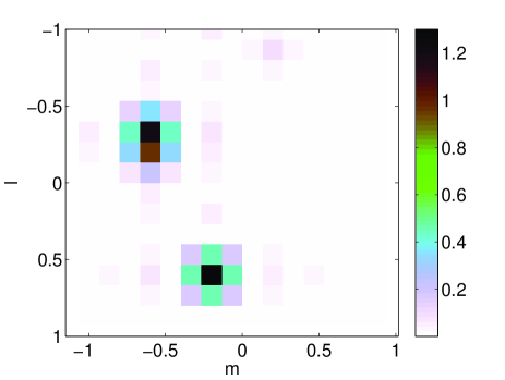
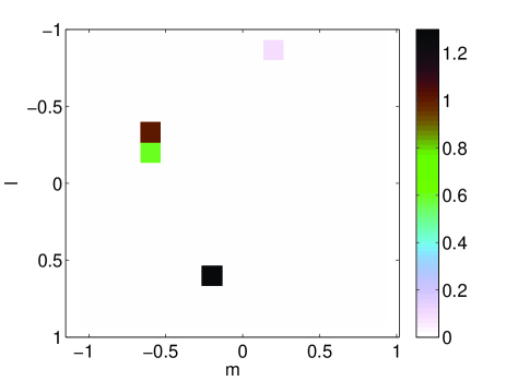
Figure 1: (a) Image obtained by normal imaging without deconvolution as in (11), showing the sources and their side lobe patterns. (b) Image obtained by model based imaging as in (22), which estimates the power at every pixel simultaneously, resulting in a deconvolved image showing only the sources without the array response.

The image value at $(l,m,n)$ is equal to the expected output power of the beamformer when pointed into that direction, and can be computed directly from the array covariance matrix $\widehat{\mathbf{R}}$ as

$$\widehat{i}\left(l,m,n\right)=\mathbf{w}^{H}\widehat{\mathbf{R}}\mathbf{w}.$$ (11)

For weights defined as in (10), this is known as direct Fourier transform imaging. To create an image, $\mathbf{w}$ is scanned over all relevant $(l,m,n)$. The required weights can be stacked into a single matrix $\mathbf{W}$. Since $\mathbf{w}^{H}\widehat{\mathbf{R}}\mathbf{w}=(\overline{\mathbf{w}}\otimes\mathbf{w})^{H}\mathrm{vec}(\widehat{\mathbf{R}})$, we can stack all image values in a single vector $\widehat{\mathbf{i}}$ and write

$$\widehat{\mathbf{i}}=(\overline{\mathbf{W}}\circ\mathbf{W})^{H}\mathrm{vec}(\widehat{\mathbf{R}}).$$ (12)

If we only want to image at the source locations, we have $\mathbf{W}=\frac{1}{p}\mathbf{A}$. A typical model assumption is that there is a source present at every pixel location, in which case

$$\widehat{\mathbf{i}}_{BF}=\frac{1}{p^{2}}(\overline{\mathbf{A}}\circ\mathbf{A})^{H}\mathrm{vec}(\widehat{\mathbf{R}}).$$ (13)

This is the classical dirty image.

Let us assume momentarily that $\mathbf{G}=\mathbf{I}$ and $\mathbf{\Sigma}_{n}=0$. Inserting the data model (6), or $\mathrm{vec}(\mathbf{R})=(\overline{\mathbf{A}}\circ\mathbf{A}){\mbox{\boldmath{$\sigma$}}}$, into (13) gives

$$\mathbf{i}_{BF} = \mathcal{E}\{\widehat{\mathbf{i}}_{BF}\}=\frac{1}{p^{2}}(\overline{\mathbf{A}}\circ\mathbf{A})^{H}(\overline{\mathbf{A}}\circ\mathbf{A}){\mbox{\boldmath{$\sigma$}}}$$ (14)

$$= \frac{1}{p^{2}}(\overline{\mathbf{A}}^{H}\overline{\mathbf{A}}\odot\mathbf{A}^{H}\mathbf{A}){\mbox{\boldmath{$\sigma$}}}$$

This shows that the dirty image is not equal to the true source structure. To understand the physical meaning of this term, consider the product $\mathbf{a}_{i}^{H}\mathbf{a}_{j}$, where the indices $i$ and $j$ refer to the respective columns of $\mathbf{A}$. Using (9) this can be written explicitly as

$$\mathbf{a}_{i}^{H}\mathbf{a}_{j} = \exp\left(-\mathrm{j}\frac{2\pi}{\lambda}\boldmath{\mathcal{R}}\mathbf{l}_{i}\right)^{H}\exp\left(-\mathrm{j}\frac{2\pi}{\lambda}\boldmath{\mathcal{R}}\mathbf{l}_{j}\right)$$ (15)

$$= \sum_{n=1}^{p}\exp\left(\mathrm{j}\frac{2\pi}{\lambda}\mathbf{r}_{n}^{T}\left(\mathbf{l}_{i}-\mathbf{l}_{j}\right)\right).$$

The physical interpretation of the inner product between the two spatial signature vectors is that it measures the sensitivity of the array to signals coming from direction $\mathbf{l}_{j}$ while the array is steered towards $\mathbf{l}_{i}$. The product $\mathbf{A}^{H}\mathbf{a}_{j}$ thus describes the array sensitivity for all directions of interest stacked in $\boldmath{\mathcal{L}}$ when pointed to $\mathbf{l}_{j}$. It therefore provides the array voltage response or array voltage beam pattern centered around $\mathbf{l}_{j}$,

$$\mathbf{b}_{V}\left(\mathbf{l}_{j}\right)=\mathbf{A}^{H}\mathbf{a}_{j}.$$ (16)

With $\mathbf{A}$ defined as in (9), this shows that the voltage beam pattern is just the Fourier transform of the spatial weighting function resulting from the array configuration and the weighting of the array elements. The corresponding power beam pattern can be calculated as

$$\mathbf{b}_{P}\left(\mathbf{l}_{j}\right)=\overline{\mathbf{b}}_{V}\left(\mathbf{l}_{j}\right)\odot\mathbf{b}_{V}\left(\mathbf{l}_{j}\right)=\overline{\mathbf{A}}^{H}\overline{\mathbf{a}}_{j}\odot\mathbf{A}^{H}\mathbf{a}_{j}.$$ (17)

The factor $\overline{\mathbf{A}}^{H}\overline{\mathbf{A}}\odot\mathbf{A}^{H}\mathbf{A}$ in (14) can thus be interpreted as a convolution by the Fourier transform of the spatial distribution of baseline vectors, which is known as the array beam pattern or dirty beam [21].

This effect is illustrated in Fig. 1($a$). This image is the result of a simulated observation with an $8\times 8$ half wavelength spaced (i.e., spatially Nyquist sampled) 2D uniform rectangular array (URA). The grid of image values on the sky is taken such that the first Nyquist zone is appropriately sampled. The underlying source model contains four sources at grid points $(-0.33,-0.6,0.73)$, $(-0.2,-0.6,0.77)$, $(0.6,-0.2,0.77)$ and $(0.87,0.2,0.46)$ respectively and ${\mbox{\boldmath{$\sigma$}}}=[1,0.6,1.3,0.1]^{T}$. This source and array configuration will be used throughout this paper unless stated otherwise. The map in Fig. 1($a$) clearly shows these four (or three, if one regards the two sources on neighboring grid points as a single extended source) being convolved with the array beam pattern.

Following a model based approach, the deconvolution problem can be formulated as a maximum likelihood (ML) estimation problem, that should provide a statistically efficient estimate of the parameters. Since all signals are assumed to be i.i.d. Gaussian signals, the derivation is standard and the ML estimates are obtained by minimizing the negative log-likelihood function [22]

$$\widehat{{\mbox{\boldmath{$\sigma$}}}}=\underset{{\mbox{\boldmath{$\sigma$}}}}{\mathrm{argmin}}\left(\ln\left|\mathbf{R}({\mbox{\boldmath{$\sigma$}}})\right|+\mathrm{tr}\left(\mathbf{R}^{-1}({\mbox{\boldmath{$\sigma$}}})\widehat{\mathbf{R}}\right)\right).$$ (18)

It does not seem possible to solve this minimization problem is closed form, but a weighted least squares covariance matching approach is known to lead to estimates that are, for a large number of samples, equivalent to ML estimates and therefore asymptotically efficient [22]. The problem can thus be reformulated as

$$\widehat{{\mbox{\boldmath{$\sigma$}}}} = \underset{{\mbox{\boldmath{$\sigma$}}}}{\mathrm{argmin}}\Big{\Arrowvert}\mathbf{W}_{c}\left(\widehat{\mathbf{R}}-{\mbox{\boldmath{$\Sigma$}}}_{n}\right)\mathbf{W}_{c}-$$ (19)

$$\mathbf{W}_{c}\mathbf{G}\mathbf{A}{\mbox{\boldmath{$\Sigma$}}}\mathbf{A}^{H}\mathbf{G}^{H}\mathbf{W}_{c}\Big{\Arrowvert}_{F}^{2}$$

$$= \underset{{\mbox{\boldmath{$\sigma$}}}}{\mathrm{argmin}}\Big{\Arrowvert}\left(\overline{\mathbf{W}}_{c}\otimes\mathbf{W}_{c}\right)\mathrm{vec}\left(\widehat{\mathbf{R}}-{\mbox{\boldmath{$\Sigma$}}}_{n}\right)-$$

$$\left(\overline{\mathbf{W}_{c}\mathbf{G}\mathbf{A}}\right)\circ\left(\mathbf{W}_{c}\mathbf{G}\mathbf{A}\right){\mbox{\boldmath{$\sigma$}}}_{n}\Big{\Arrowvert}_{F}^{2}$$

The solution is given by

$$\widehat{\mbox{\boldmath{$\sigma$}}}=\left(\left(\overline{\mathbf{W}_{c}\mathbf{G}\mathbf{A}}\right)\circ\left(\mathbf{W}_{c}\mathbf{G}\mathbf{A}\right)\right)^{\dagger}\left(\overline{\mathbf{W}}_{c}\otimes\mathbf{W}_{c}\right)\mathrm{vec}\left(\widehat{\mathbf{R}}-{\mbox{\boldmath{$\Sigma$}}}_{n}\right)$$ (20)

Optimal weighting is provided by $\mathbf{W}_{c}=\mathbf{R}^{-\frac{1}{2}}$. Since radio astronomical sources are generally very weak with the strongest source in the field having an instantaneous SNR in the order of 0.01, we can introduce the approximation $\mathbf{R}\approx\sigma_{n}^{2}\mathbf{I}$ for an array of identical elements for convenience of notation. This reduces (20) to

$$\widehat{{\mbox{\boldmath{$\sigma$}}}} = \left(\overline{\mathbf{GA}}\circ\mathbf{GA}\right)^{\dagger}\mathrm{vec}\left(\widehat{\mathbf{R}}-{\mbox{\boldmath{$\Sigma$}}}_{n}\right).$$ (21)

One may argue that this requires one to know where the sources are before doing the imaging. This is generally solved by simultaneously estimating the source locations and source powers. Although the CLEAN algorithm has not yet been fully analyzed, it can be regarded as an iterative procedure to do this [11]. It is instructive, however, to use (21) for imaging by estimating the power on every image point (pixel), i.e., by assuming a data model with a source present at every pixel. We can simplify (21) by replacing the Moore-Penrose pseudo-inverse by the left pseudo-inverse, to obtain the image vector

$$\widehat{\mathbf{i}} = \left(\left(\overline{\mathbf{GA}}\circ\mathbf{GA}\right)^{H}\left(\overline{\mathbf{GA}}\circ\mathbf{GA}\right)\right)^{-1}\times$$ (22)

$$\times\left(\overline{\mathbf{GA}}\circ\mathbf{GA}\right)^{H}\mathrm{vec}\left(\widehat{\mathbf{R}}-{\mbox{\boldmath{$\Sigma$}}}_{n}\right)$$

$$= \left(\overline{\mathbf{A}}^{H}{\mbox{\boldmath{$\Gamma$}}}^{2}\overline{\mathbf{A}}\odot\mathbf{A}^{H}{\mbox{\boldmath{$\Gamma$}}}^{2}\mathbf{A}\right)^{-1}\times$$

$$\times\left(\overline{\mathbf{GA}}\circ\mathbf{GA}\right)^{H}\mathrm{vec}\left(\widehat{\mathbf{R}}-{\mbox{\boldmath{$\Sigma$}}}_{n}\right).$$

The first factor in this equation represents the deconvolution operation. It is therefore convenient to introduce the deconvolution matrix $\mathbf{M}=\overline{\mathbf{A}}^{H}{\mbox{\boldmath{$\Gamma$}}}^{2}\overline{\mathbf{A}}\odot\mathbf{A}^{H}{\mbox{\boldmath{$\Gamma$}}}^{2}\mathbf{A}=\left|\mathbf{A}^{H}{\mbox{\boldmath{$\Gamma$}}}^{2}\mathbf{A}\right|^{\odot 2}$. This provides a powerful check on the sampling of the image plane. If the image plane is oversampled, i.e., if too many image points are defined, this matrix will be singular. This property demonstrates that high resolution imaging is only possible if a limited number of sources is present, i.e., if the number of sources is much smaller than the number of resolution elements in the field-of-view. The condition number of the deconvolution matrix, which provides a measure on the magnification of measurement noise, is discussed in more detail in Sec. III-C. This mostly empty field-of-view is commonly assumed in astronomical imaging and this assumption is one of the reasons why CLEAN and MEM work in practice. Fig. 1($b$) shows the image obtained by applying (22) to the $8\times 8$ URA. Comparison with the image obtained using (13) clearly shows the effectiveness of the model based imaging approach in suppressing the array beam pattern.

III-B Noise redistribution

If imaging is done without deconvolution by using (13), the thermal noise adds a constant value to all image values. This can be illustrated by assuming that $\mathcal{E}\left\{\widehat{\mathbf{R}}\right\}={\mbox{\boldmath{$\Sigma$}}}_{n}$, i.e. by assuming that the image is completely dominated by thermal noise. The expected value of the image then becomes

$$\mathbf{i}_{BF} = \frac{1}{p^{2}}\left(\overline{\mathbf{A}}\circ\mathbf{A}\right)^{H}\mathrm{vec}\left({\mbox{\boldmath{$\Sigma$}}}_{n}\right)$$ (23)

$$= \frac{1}{p^{2}}\left(\overline{\mathbf{A}}\odot\mathbf{A}\right)^{H}{\mbox{\boldmath{$\sigma$}}}_{n}$$

$$= \frac{\mathbf{1}^{T}{\mbox{\boldmath{$\sigma$}}}_{n}}{p^{2}}\mathbf{1}$$

where we used the fact that all elements of $\mathbf{A}$ have unit amplitude. This equation describes an image where all values are equal to the average thermal noise per baseline.

If the imaging process involves deconvolution, the result is described by (22). For simplicity we will assume that we have an array of identical elements, so that we can set $\mathbf{G}=\mathbf{I}$. Further, to illustrate the effect, we momentarily omit the correction by $\mathbf{\Sigma}_{n}$ in (22). In this case, the expected value of the image is

$$\mathbf{i} = \left(\overline{\mathbf{A}}^{H}\overline{\mathbf{A}}\odot\mathbf{A}^{H}\mathbf{A}\right)^{-1}\left(\overline{\mathbf{A}}\circ\mathbf{A}\right)^{H}{\mbox{\boldmath{$\Sigma$}}}_{n}$$ (24)

$$= \left(\left|\mathbf{A}^{H}\mathbf{A}\right|^{\odot 2}\right)^{-1}\left(\overline{\mathbf{A}}\odot\mathbf{A}\right)^{H}{\mbox{\boldmath{$\sigma$}}}_{n}$$

$$= \left(\left|\mathbf{A}^{H}\mathbf{A}\right|^{\odot 2}\right)^{-1}\left(\mathbf{1}^{T}{\mbox{\boldmath{$\sigma$}}}_{n}\right)\mathbf{1}.$$

In this case, the homogeneity of the thermal noise distribution in the map depends on the row sums of $\left(\left|\mathbf{A}^{H}\mathbf{A}\right|^{\odot 2}\right)^{-1}$ being constant. If this is true, the model based image using (22) is analogous to the beamformed image based on (13). A special case is the situation in which the columns of $\mathbf{A}$ are orthonormal.

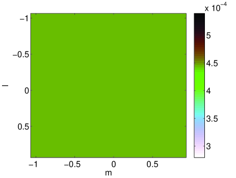
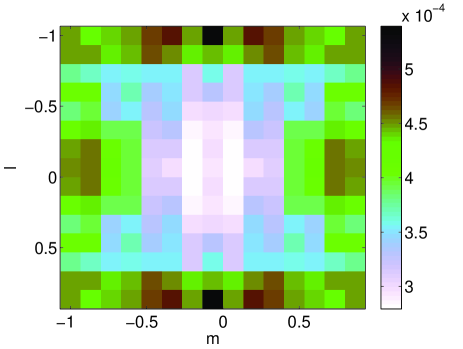
Figure 2: ($a$) Imaging with deconvolution using an $8\times 8$ half wavelength spaced array for a Nyquist sampled image assuming $\mathbf{R}=0.1\mathbf{I}$ (an empty field with only thermal noise). ($b$) Imaging result for a five armed array, each arm being an eight element half wavelength spaced ULA.

Otherwise, the structure is more complicated. This is illustrated in Fig. 2 which compares the noise distribution in the image plane of the $8\times 8$ URA by assuming $\mathbf{R}=0.1\mathbf{I}$ with the corresponding image for a five armed array, each arm being an eight element half wavelength spaced Uniform Linear Array (ULA). The impact of the redistribution of noise can be reduced by estimating the receiver noise powers and subtracting these estimates from the array covariance matrix as described by (22). In most astronomical imaging algorithms, the autocorrelations are generally ignored completely thus effectively introducing a small negative system noise since the autocorrelations represent the power sum of the source signals and the noise.

III-C Deconvolution matrix condition number

The deconvolution matrix $\mathbf{M}$ not only causes a redistribution of noise over the map, but also determines whether the deconvolution is a well conditioned problem. If the deconvolution matrix is not invertible, the problem is ill-posed and additional constraints are required to obtain a unique solution. Different choices for these constraints or even the rigor with which they are applied, lead to different imaging results for CLEAN and MEM based on the same data. In some cases, this may even lead to different interpretation of the final maps [14]. These problems arise due to over-interpretation of the data by allowing for more image points (parameters) than can be justified by the data. In these situations, the condition number of the deconvolution matrix will be infinitely large. Even if the deconvolution matrix is invertible, its condition number may be unacceptably high in view of the SNR of the data: the condition number is a measure for the magnification of measurement noise [23]. The condition number thus provides a powerful diagnostic tool to assess the feasibility of the deconvolution problem at hand.

It is instructive to analyze a half wavelength spaced 1D ULA with identical elements, i.e. with $\mathbf{G}=\mathbf{I}$, sampling the sky on a regular grid. In this case $\mathbf{A}$ represents a Fourier transform mapping the spatial frequencies on the sky to the spatial samples describing the electromagnetic field over the array aperture. As demonstrated in the previous section, these spatial frequencies will be convolved in the imaging process with the Fourier transform of the array aperture taper or voltage beam pattern, which can be easily calculated for $\mathbf{l}=\mathbf{0}$:

$$\mathbf{b}_{V}\left(\mathbf{0}\right)=\mathbf{A}^{H}\mathbf{a}(\mathbf{0})=\mathcal{FT}\left(\left[\begin{array}[]{@{}c@{}}\mathbf{1}_{p}\\ \mathbf{0}_{n-p}\end{array}\right]\right).$$ (25)

Here $\cal{FT}$ denotes the Fourier transform, $n$ is the total number of image points, $p$ is the number of elements in the array and $\mathbf{0}_{p}$ and $\mathbf{1}_{p}$ denote $p\times 1$ vectors containing zeros and ones respectively. The corresponding power beam pattern is

$$\mathbf{b}_{P}\left(\mathbf{0}\right) = \overline{\mathbf{b}}_{V}\left(\mathbf{0}\right)\odot\mathbf{b}_{V}\left(\mathbf{0}\right)$$ (30)

$$= \mathcal{FT}\left(\left[\begin{array}[]{@{}c@{}}\mathbf{1}_{p}\\ \mathbf{0}_{n-p}\end{array}\right]\circledast\left[\begin{array}[]{@{}c@{}}\mathbf{1}_{p}\\ \mathbf{0}_{n-p}\end{array}\right]\right).$$

If the columns of $\mathbf{A}$ are ordered such that they describe the array response vectors for the regularly spaced DOAs starting with $\mathbf{l}_{1}=\mathbf{0}$, it is easily seen that

$$\mathbf{M}=\overline{\mathbf{A}}^{H}\overline{\mathbf{A}}\odot\mathbf{A}^{H}\mathbf{A}=\mathrm{circulant}\left(\mathbf{b}_{P}\left(\mathbf{0}\right)\right),$$ (31)

i.e., that the deconvolution matrix for a 1D ULA equidistantly sampling the image plane is a circulant matrix. Since $\mathbf{M}$ is a circulant matrix, its eigenvalues ${\mbox{\boldmath{$\lambda$}}}=[\lambda_{1},\lambda_{2},\cdots,\lambda_{n}]^{T}$ are given by the Fourier transform of $\mathbf{b}_{P}(\mathbf{0})$ [24], or

$$\lambda = \mathcal{FT}\left(\mathbf{b}_{P}(\mathbf{0})\right)$$ (36)

$$= \mathcal{FT}\left(\mathcal{FT}\left(\left[\begin{array}[]{@{}c@{}}\mathbf{1}_{p}\\ \mathbf{0}_{n-p}\end{array}\right]\circledast\left[\begin{array}[]{@{}c@{}}\mathbf{1}_{p}\\ \mathbf{0}_{n-p}\end{array}\right]\right)\right)$$

$$= \left[\begin{array}[]{@{}c@{}}\mathbf{1}_{p}\\ \mathbf{0}_{n-p}\end{array}\right]\circledast\left[\begin{array}[]{@{}c@{}}\mathbf{1}_{p}\\ \mathbf{0}_{n-p}\end{array}\right]$$ (41)

since $\mathcal{FT}(\cdot)=\mathcal{FT}^{-1}(\cdot)$ for real symmetric functions.

For Hermitian matrices, the condition number $\kappa$ is given by the ratio of the largest and smallest eigenvalue, i.e. $\kappa=\lambda_{max}/\lambda_{min}$ [24]. If the image plane is Nyquist sampled, $n=2p-1$ and

$${\mbox{\boldmath{$\lambda$}}}=\left[1,2,\cdots,p-1,p,p-1,\cdots,2,1\right]^{T}.$$ (42)

In this case the condition number of $\mathbf{M}$ is

$$\kappa=\frac{\lambda_{max}}{\lambda_{min}}=\frac{p}{1}=p,$$ (43)

thus $\mathbf{M}$ is invertible. The deconvolution problem is therefore well-posed and has a unique solution.

If the image plane is undersampled with $n<2p-1$ samples, then

$${\mbox{\boldmath{$\lambda$}}}=\left[p-\frac{n-1}{2},\cdots,p-1,p,p-1,\cdots,p-\frac{n-1}{2}\right]^{T}$$ (44)

and $\kappa=\frac{2p}{2p-(n-1)}$. The deconvolution problem in itself is thus well-posed and has a unique solution. However, from Fourier theory we know that aliasing effects may occur due to undersampling.

If the image plane is oversampled with $n>2p-1$ samples, then

$${\mbox{\boldmath{$\lambda$}}}=\left[\cdots,0,1,2,\cdots,p-1,p,p-1,\cdots,2,1,0,\cdots\right]^{T}$$ (45)

and $\kappa=\infty$. In this case, the deconvolution problem is ill-posed and thus not solvable without introducing additional boundary conditions to constrain the problem.

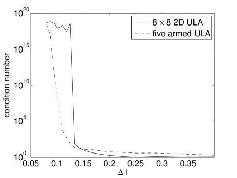
Figure 3: This plot shows the condition number of the deconvolution matrix as function of the image resolution for the $8\times 8$ half wavelength spaced array and the five armed array with each arm being an eight element half wavelength spaced ULA.

This analysis shows that, for a 1D ULA, the condition number slowly increases up to Nyquist sampling of the image plane and then jumps to infinity. Since a URA is just the 2D analog of a 1D ULA, this behavior is also expected for the $8\times 8$ URA introduced earlier. This conjecture is confirmed in Fig. 3 which shows the condition number of the deconvolution matrix as function of image resolution. This figure also shows the corresponding curve for the five armed array introduced earlier to demonstrate the impact of less regular and sparser sampling of the array aperture. Although the array diameter is nearly twice as large, it does not provide twice the resolution due to sparser sampling of the aperture plane. This plot also demonstrates that a less regular array also may have a less strict cut-off: the transition of the condition number from small values to infinity is a gradual one. For array processing problems, this means that the user should decide which value of the condition number (or noise enhancement) is still acceptable.

Regularization is commonly used to avoid uninvertability of matrices. In radio astronomical imaging where most sources have a low SNR, this would lead to imperfect deconvolution causing the weakest sources in the field to be drowned in the imperfectly removed array response pattern of the strongest sources. However, several forms of implicit regularization have been studied to handle special cases like strong interference [25].

IV Effective noise

Equation (22) shows that calibration and imaging are strongly coupled. Knowledge of the instrumental parameters is required to obtain the proper image. People have approached this problem in two ways. In the first approach calibration and imaging are treated as separate steps, i.e., the instrumental parameters are estimated first by a calibration measurement and consecutively applied to the actual measurement data. The second approach is self calibration which regards the estimation of instrumental and image parameters as a single parameter estimation problem [26, 27, 28, 13].

In either case the achievable dynamic range is limited by the combination of estimation errors, thermal noise and confusion noise. Together, they determine the effective noise in the image which need not be homogeneous over the field of interest. In this section a number of analytical expressions are derived that describe these contributions in terms of the data model presented in Section II. The implications will be discussed in Section V.

IV-A Noise in self calibrated images

In self calibration the instrumental and image parameters are estimated simultaneously. Self calibration based on the data model presented above can thus be described as simultaneous estimation of the omni-directional complex gains, the apparent source powers, the source locations and the receiver noise powers, i.e., of a parameter vector

$$\theta = [\gamma_{1},\cdots,\gamma_{p},\phi_{2},\cdots,\phi_{p},\sigma_{2}^{2},\cdots,\sigma_{q}^{2},\sigma_{n1}^{2},\cdots,\sigma_{np}^{2},$$

$$\ l_{2},\cdots,l_{q},m_{2},\cdots,m_{q}]^{T}.$$

In this parameter vector, $\phi_{1}$ and $\sigma_{1}^{2}$ are omitted because they are set to constants for the problem to be identifiable. Indeed, the restriction $\sigma_{1}^{2}=1$ is imposed by the fact that $\mathbf{G}$ and $\Sigma$ share a common factor, while the first constraint is required since one can only measure the gain phases with respect to some reference, here achieved by setting $\phi_{1}=0$.

Similarly to (19), the parameters are obtained by solving

$$\widehat{{\mbox{\boldmath{$\theta$}}}}=\underset{{\mbox{\boldmath{$\theta$}}}}{\mathrm{argmin}}\parallel\mathbf{W}_{c}\left(\widehat{\mathbf{R}}-\mathbf{GA}{\mbox{\boldmath{$\Sigma$}}}\mathbf{A}^{H}\mathbf{G}^{H}-{\mbox{\boldmath{$\Sigma$}}}_{n}\right)\mathbf{W}_{c}\parallel_{F}^{2},$$ (46)

where $\mathbf{G}$, $\mathbf{A}$, $\mathbf{\Sigma}$ and $\mathbf{\Sigma}_{n}$ are all functions of $\theta$ and $\mathbf{W}_{c}=\mathbf{R}^{-\frac{1}{2}}\approx\frac{1}{\sigma_{n}}\mathbf{I}$ as argued earlier.

The minimum variance for an unbiased estimator is given by the Cramèr-Rao Bound (CRB). The CRB on the error variance for any unbiased estimator states that the covariance matrix $\mathbf{C}_{\theta}$ of the parameter vector $\theta$ satisfies [30]

$$\mathbf{C}_{\theta}=\mathcal{E}\left\{\left(\widehat{{\mbox{\boldmath{$\theta$}}}}-{\mbox{\boldmath{$\theta$}}}\right)\left(\widehat{{\mbox{\boldmath{$\theta$}}}}-{\mbox{\boldmath{$\theta$}}}\right)^{T}\right\}\geq\frac{1}{N}\mathbf{J}^{-1},$$ (47)

where $\mathbf{J}$ is the Fisher information matrix (FIM). For Gaussian data models $\mathbf{J}$ can be expressed as (e.g. [31])

$$\mathbf{J}=\mathbf{F}^{H}\left(\overline{\mathbf{R}}^{-1}\otimes\mathbf{R}^{-1}\right)\mathbf{F}$$ (48)

where $\mathbf{R}$ is the data covariance matrix and $\mathbf{F}$ is the Jacobian evaluated at the true values of the parameters, i.e.,

$$\mathbf{F}=\frac{\delta\mathrm{vec}(\mathbf{R})}{\delta{\mbox{\boldmath{$\theta$}}}^{T}}\Big{|}_{{\mbox{\boldmath{$\theta$}}}}.$$ (49)

For the self calibration scenario, the Jacobian can be partitioned into six parts following the structure of $\theta$:

$$\mathbf{F}=[\mathbf{F}_{\gamma},\mathbf{F}_{\phi},\mathbf{F}_{\sigma},\mathbf{F}_{\sigma_{n}},\mathbf{F}_{l},\mathbf{F}_{m}].$$ (50)

By substitution of (8) in (49), it follows directly that the first four components can be expressed as

$$\mathbf{F}_{\gamma} = \left(\overline{\mathbf{G}\mathbf{R}_{0}}{\mbox{\boldmath{$\Phi$}}}\right)\circ\mathbf{I}+\mathbf{I}\circ\left(\mathbf{G}\mathbf{R}_{0}\overline{{\mbox{\boldmath{$\Phi$}}}}\right)$$ (51)

$$\mathbf{F}_{\phi} = \mathrm{j}\left(\left(\overline{\mathbf{G}\mathbf{R}_{0}}\mathbf{G}\right)\circ\mathbf{I}-\mathbf{I}\circ\left(\mathbf{G}\mathbf{R}_{0}\overline{\mathbf{G}}\right)\right)\mathbf{I}_{s}$$ (52)

$$\mathbf{F}_{\sigma} = \left(\left(\overline{\mathbf{G}\mathbf{A}}\right)\circ\left(\mathbf{G}\mathbf{A}\right)\right)\mathbf{I}_{s}$$ (53)

$$\mathbf{F}_{\sigma_{n}} = \mathbf{I}\circ\mathbf{I}$$ (54)

where $\mathbf{R}_{0}=\mathbf{A}{\mbox{\boldmath{$\Sigma$}}}\mathbf{A}^{H}$ and $\mathbf{I}_{s}$ is a selection matrix of appropriate size equal to the identity matrix with its first column removed so that the derivatives with respect to $\phi_{1}$ and $\sigma_{1}^{2}$ are omitted.

If the receiver noise powers of all $p$ elements are the same, the expression for $\mathbf{F}_{\sigma_{n}}$ given in (54) should be replaced by

$$\mathbf{F}_{\sigma_{n}}=\mathrm{vec}(\mathbf{I})$$ (55)

For the last two components of the FIM, derivatives of $\mathrm{vec}\left(\mathbf{R}\right)$ with respect to the source position coordinates are required. Let $(x_{i},y_{i})$ be the coordinates of the $i$th array element, and introduce

$$\mathbf{G}_{x} = \mathrm{diag}([x_{1},x_{2},\cdots x_{p}]^{T})\mathbf{G}$$ (56)

$$\mathbf{G}_{y} = \mathrm{diag}([y_{1},y_{2},\cdots y_{p}]^{T})\mathbf{G}$$ (57)

then these components can be conveniently written as

$$\mathbf{F}_{l} = -\mathrm{j}\frac{2\pi}{\lambda}\left(\overline{\mathbf{G}\mathbf{A}}\circ\mathbf{G}_{x}\mathbf{A}-\overline{\mathbf{G}_{x}\mathbf{A}}\circ\mathbf{G}\mathbf{A}\right){\mbox{\boldmath{$\Sigma$}}}\mathbf{I}_{s}$$ (58)

$$\mathbf{F}_{m} = -\mathrm{j}\frac{2\pi}{\lambda}\left(\overline{\mathbf{G}\mathbf{A}}\circ\mathbf{G}_{y}\mathbf{A}-\overline{\mathbf{G}_{y}\mathbf{A}}\circ\mathbf{G}\mathbf{A}\right){\mbox{\boldmath{$\Sigma$}}}\mathbf{I}_{s}$$ (59)

These equations show that the entries of the Jacobian related to derivatives with respect to the $l$- and $m$-coordinates of the sources are proportional to the $x$- and $y$-coordinates of the array elements respectively. The physical interpretation of this relation is that a plane wave propagating along the coordinate axis of the coordinate to be estimated provides a more useful test signal to estimate the source location than a signal propagating perpendicular to this axis.

The preceding equations allow us to compute $\mathbf{C}_{\theta}$. The variance of the estimated image values, i.e. the noise on the image values due to estimation inaccuracy, is given by the diagonal of the sub-block $\mathbf{C}_{\sigma\sigma}$ of this matrix, following the partitioning of $\theta$. In general $\mathbf{C}_{\sigma\sigma}$ is not a diagonal matrix. The other entries in this sub-block describe the way in which the noise on the pixels are correlated among themselves—this is associated with false structures.

IV-B Propagation of calibration errors

If the instrumental parameters are extracted from separate calibration data, the minimum variance on these estimated values is given by the CRB on the instrumental parameters in the calibration experiment, $\mathbf{C}_{\theta}$, where now ${\mbox{\boldmath{$\theta$}}}=[\gamma_{1},\cdots,\gamma_{p},\phi_{2},\cdots,\phi_{p},\sigma_{n1}^{2},\cdots,\sigma_{np}^{2}]^{T}$. With this choice for $\theta$ the results for $\mathbf{F}_{\gamma}$, $\mathbf{F}_{\phi}$ and $\mathbf{F}_{\sigma_{n}}$ derived earlier in (51), (52) and (54) can be used assuming that the calibration measurement adheres to the same data model. The propagation of the calibration errors to the image is described by

$$\mathrm{cov}\left(\mathbf{i}\right)=\left(\frac{\partial\mathbf{i}}{\partial{\mbox{\boldmath{$\theta$}}}^{T}}\right)\mathbf{C}_{\theta}\left(\frac{\partial\mathbf{i}}{\partial{\mbox{\boldmath{$\theta$}}}^{T}}\right)^{T}.$$ (60)

We thus need to derive $\partial\mathbf{i}/\partial{\mbox{\boldmath{$\gamma$}}}^{T}$, $\partial\mathbf{i}/\partial{\mbox{\boldmath{$\phi$}}}^{T}$ and $\partial\mathbf{i}/\partial{\mbox{\boldmath{$\sigma$}}}_{n}^{T}$.

The derivative of the image values to $\gamma_{k}$ is defined as

$$\frac{\partial\mathbf{i}}{\partial\gamma_{k}}=\frac{\partial}{\partial\gamma_{k}}\mathbf{M}^{-1}\left(\overline{\mathbf{GA}}\circ\mathbf{GA}\right)^{H}\mathrm{vec}\left(\mathbf{R}-{\mbox{\boldmath{$\Sigma$}}}_{n}\right)$$ (61)

where $\mathbf{M}$ and $\mathbf{G}$ depend on $\mathbf{\gamma}$. Applying the formula for the derivative of an inverted matrix with respect to one of its elements [24], this can be rewritten as

$$\frac{\partial\mathbf{i}}{\partial\gamma_{k}}=$$ (62)

$$=\Bigg{(}-\mathbf{M}^{-1}\left(\frac{\partial}{\partial\gamma_{k}}\mathbf{M}\right)\mathbf{M}^{-1}\left(\overline{\mathbf{GA}}\circ\mathbf{GA}\right)^{H}+$$

$$+\mathbf{M}^{-1}\gamma_{k}\left(\mathrm{e}^{-\mathrm{j}\phi_{k}}\mathbf{E}_{kk}\overline{\mathbf{A}}\circ\mathbf{GA}+\overline{\mathbf{GA}}\circ\mathrm{e}^{\mathrm{j}\phi_{k}}\mathbf{E}_{kk}\mathbf{A}\right)^{H}\Bigg{)}$$

$$\times\mathrm{vec}\left(\mathbf{R}-{\mbox{\boldmath{$\Sigma$}}}_{n}\right)$$

where $\mathbf{E}_{kk}$ is the elementary matrix with all its entries set to zero except element $E_{kk}$ which is set to 1. Inserting the vectorized version of (8) in (62) and removing the Khatri-Rao products, we obtain

$$\frac{\partial\mathbf{i}}{\partial\gamma_{k}}=-2\gamma_{k}\left(2-\gamma_{k}\right)\mathbf{M}^{-1}\mathrm{Re}\left\{\overline{\mathbf{A}}_{k:}^{H}\overline{\mathbf{A}}_{k:}\odot\mathbf{A}^{H}{\mbox{\boldmath{$\Gamma$}}}^{2}\mathbf{A}\right\}{\mbox{\boldmath{$\sigma$}}}$$ (63)

We have introduced the notation $\mathbf{A}_{k:}=\mathbf{E}_{kk}\mathbf{A}$, i.e. $\mathbf{A}_{k:}$ has only zero valued entries except on the $k$th row where the elements are equal to the corresponding elements of $\mathbf{A}$. The goal of this derivation is to obtain an expression for $\partial\mathbf{i}/\partial{\mbox{\boldmath{$\gamma$}}}^{T}$. We will thus have to stack the expression for $\partial\mathbf{i}/\partial\gamma_{k}$ in a single matrix. This is facilitated by introducing $\mathbf{a}_{k}$ as the $k$th row of $\mathbf{A}$ and rewriting (63) as

$$\frac{\partial\mathbf{i}}{\partial\gamma_{k}}=-2\gamma_{k}\left(2-\gamma_{k}\right)\mathbf{M}^{-1}\mathrm{Re}\left\{\mathbf{a}_{k}^{T}\mathbf{1}^{T}\odot\mathbf{A}^{H}{\mbox{\boldmath{$\Gamma$}}}^{2}\mathbf{A}{\mbox{\boldmath{$\Sigma$}}}\mathbf{a}_{k}^{H}\right\}$$ (64)

where $\mathbf{1}$ denotes a vector of ones of appropriate size.

By stacking all vector $\partial\mathbf{i}/\partial\gamma_{k}$ in a single matrix, we thus obtain

$$\frac{\partial\mathbf{i}}{\partial{\mbox{\boldmath{$\gamma$}}}^{T}}=-2\mathbf{M}^{-1}\mathrm{Re}\left\{\mathbf{A}^{T}\odot\mathbf{A}^{H}{\mbox{\boldmath{$\Gamma$}}}^{2}\mathbf{A}{\mbox{\boldmath{$\Sigma$}}}\mathbf{A}^{H}\right\}\left(2\mathbf{I}-{\mbox{\boldmath{$\Gamma$}}}\right){\mbox{\boldmath{$\Gamma$}}}.$$ (65)

The corresponding result for $\phi_{k}$ can be derived in a similar way, so we only present the main steps.

$$\frac{\partial\mathbf{i}}{\partial\phi_{k}}=$$ (66)

$$= \frac{\partial}{\partial\phi_{k}}\left(\overline{\mathbf{G}\mathbf{A}}\circ\mathbf{G}\mathbf{A}\right)^{\dagger}\mathrm{vec}\left(\mathbf{R}\right)$$

$$= \mathbf{M}^{-1}\left(\frac{\partial}{\partial\phi_{k}}\overline{\mathbf{GA}}\circ\mathbf{GA}\right)^{H}\left(\left(\overline{\mathbf{G}\mathbf{A}}\circ\mathbf{G}\mathbf{A}\right)^{H}{\mbox{\boldmath{$\sigma$}}}\right)$$

$$= \mathbf{M}^{-1}\left(-\mathrm{j}\mathrm{e}^{-\mathrm{j}\phi_{k}}{\mbox{\boldmath{$\Gamma$}}}\overline{\mathbf{A}}_{k:}\circ\mathbf{GA}+\mathrm{j}\mathrm{e}^{\mathrm{j}\phi_{k}}\overline{\mathbf{GA}}\circ{\mbox{\boldmath{$\Gamma$}}}\mathbf{A}_{k:}\right)^{H}$$

$$\times\left(\left(\overline{\mathbf{G}\mathbf{A}}\circ\mathbf{G}\mathbf{A}\right)^{H}{\mbox{\boldmath{$\sigma$}}}\right).$$

Removal of the Khatri-Rao products by reducing them to Hadamard products gives

$$\frac{\partial\mathbf{i}}{\partial\phi_{k}} = -2\gamma_{k}^{2}\mathbf{M}^{-1}\mathrm{Im}\left\{\left(\overline{\mathbf{A}}_{k:}^{H}\overline{\mathbf{A}_{k:}}\odot\mathbf{A}^{H}{\mbox{\boldmath{$\Gamma$}}}^{2}\mathbf{A}\right)\right\}{\mbox{\boldmath{$\sigma$}}}.$$ (67)

Note that this term has the same form as the first term in (63), so it can be rewritten in a similar way. This gives

$$\frac{\partial\mathbf{i}}{\partial\phi_{k}}=-2\gamma_{k}^{2}\mathbf{M}^{-1}\mathrm{Im}\left\{\mathbf{a}_{k}^{T}\mathbf{1}^{T}\odot\mathbf{A}^{H}{\mbox{\boldmath{$\Gamma$}}}^{2}\mathbf{A}{\mbox{\boldmath{$\Sigma$}}}\mathbf{a}_{k}^{H}\right\}$$ (68)

and therefore

$$\frac{\partial\mathbf{i}}{\partial{\mbox{\boldmath{$\phi$}}}^{T}}=-2\mathbf{M}^{-1}\mathrm{Im}\left\{\overline{\mathbf{A}}^{H}\odot\mathbf{A}^{H}{\mbox{\boldmath{$\Gamma$}}}^{2}\mathbf{A}{\mbox{\boldmath{$\Sigma$}}}\mathbf{A}^{H}\right\}{\mbox{\boldmath{$\Gamma$}}}^{2}$$ (69)

Finally, the partial derivative of the image values with respect to $(\sigma_{nk}^{2})$ is given by

$$\frac{\partial\mathbf{i}}{\partial(\sigma_{nk}^{2})} = \frac{\partial}{\partial(\sigma_{nk}^{2})}\mathbf{M}^{-1}\left(\overline{\mathbf{GA}}\circ\mathbf{GA}\right)^{H}\mathrm{vec}\left(\mathbf{R}-{\mbox{\boldmath{$\Sigma$}}}_{n}\right)$$ (70)

$$= \mathbf{M}^{-1}\left(\overline{\mathbf{GA}}\circ\mathbf{GA}\right)^{H}\mathrm{vec}\left(-\mathbf{E}_{kk}\right)$$

$$= -\mathbf{M}^{-1}\left(\left|\mathbf{GA}\right|^{\odot 2}\right)^{H}\mathrm{vecdiag}\left(\mathbf{E}_{kk}\right).$$

Therefore

$$\frac{\partial\mathbf{i}}{\partial{\mbox{\boldmath{$\sigma$}}}_{n}^{T}}=-\mathbf{M}^{-1}\left(\left|\mathbf{GA}\right|^{\odot 2}\right)^{H}.$$ (71)

If ${\mbox{\boldmath{$\Sigma$}}}_{n}=\sigma_{n}^{2}\mathbf{I}$ this reduces further to

$$\frac{\partial\mathbf{i}}{\partial\sigma_{n}}=-\mathbf{M}^{-1}\left(\left|\mathbf{GA}\right|^{\odot 2}\right)^{H}\mathbf{1}.$$ (72)

The partial derivatives as well as the CRB [19] contain terms involving $\mathbf{A}^{H}\mathbf{A}$, often weighted by the gains of the receiving elements. Given the physical interpretation of this factor discussed in section III, this suggests that the error patterns introduced in the image by calibration errors follow the structures in the dirty image. This is confirmed by the example in section V. Since the CRB is inversely proportional with $N$, which is equal to the product of bandwidth and integration time, the image covariance due to calibration errors decreases proportional to bandwidth and integration time.

IV-C Thermal noise

In this section we derive an expression for the covariance of the image values due to the thermal noise in the data. We will therefore assume that perfect knowledge of the thermal noise power ${\mbox{\boldmath{$\Sigma$}}}_{n}$ is available to avoid confusion between the thermal noise contribution and the contribution of propagated estimation errors. The covariance of the image values is by definition given by

$$\mathrm{cov}\left(\mathbf{i}\right)=$$ (73)

$$= \mathcal{E}\left\{\left(\mathrm{vec}\left(\widehat{\mathbf{i}}\right)-\mathrm{vec}\left(\mathbf{i}\right)\right)\left(\mathrm{vec}\left(\widehat{\mathbf{i}}\right)-\mathrm{vec}\left(\mathbf{i}\right)\right)^{H}\right\}$$

$$= \mathcal{E}\Big{\{}\left(\overline{\mathbf{GA}}\circ\mathbf{GA}\right)^{\dagger}\left(\mathrm{vec}\left(\widehat{\mathbf{R}}-{\mbox{\boldmath{$\Sigma$}}}_{n}\right)-\mathrm{vec}\left(\mathbf{R}-{\mbox{\boldmath{$\Sigma$}}}_{n}\right)\right)$$

$$\times\left(\mathrm{vec}\left(\widehat{\mathbf{R}}-{\mbox{\boldmath{$\Sigma$}}}_{n}\right)-\mathrm{vec}\left(\mathbf{R}-{\mbox{\boldmath{$\Sigma$}}}_{n}\right)\right)^{H}$$

$$\times\left(\overline{\mathbf{GA}}\circ\mathbf{GA}\right)^{\dagger H}\Big{\}}.$$

This shows that under the assumption that perfect knowledge on ${\mbox{\boldmath{$\Sigma$}}}_{n}$ in $\widehat{\mathbf{R}}$ is available, ${\mbox{\boldmath{$\Sigma$}}}_{n}$ drops out. Furthermore, $(\overline{\mathbf{GA}}\circ\mathbf{GA})^{\dagger}$ can be moved outside the expectation operator, since it contains no estimated values. Therefore

$$\mathrm{cov}\left(\mathbf{i}\right)=\mathbf{M}^{-1}\left(\overline{\mathbf{GA}}\circ\mathbf{GA}\right)^{H}\mathrm{cov}\left(\mathbf{R}\right)\left(\overline{\mathbf{GA}}\circ\mathbf{GA}\right)\mathbf{M}^{-1}.$$ (74)

For Gaussian data models

$$\mathrm{cov}\left(\mathbf{R}\right)=\frac{1}{N}\left(\overline{\mathbf{R}}\otimes\mathbf{R}\right),$$ (75)

and we find that

$$\mathrm{cov}\left(\mathbf{i}\right)=$$

$$= \frac{1}{N}\mathbf{M}^{-1}\left(\overline{\mathbf{GA}}\circ\mathbf{GA}\right)^{H}\left(\overline{\mathbf{R}}\otimes\mathbf{R}\right)\left(\overline{\mathbf{GA}}\circ\mathbf{GA}\right)\mathbf{M}^{-1}.$$

This can be rewritten using Kronecker and Khatri-Rao product relations as

$$\mathrm{cov}\left(\mathbf{i}\right) = \frac{1}{N}\mathbf{M}^{-1}\left(\overline{\mathbf{GA}}\circ\mathbf{GA}\right)^{H}\left(\overline{\mathbf{RGA}}\circ\mathbf{RGA}\right)\mathbf{M}^{-1}$$ (76)

$$= \frac{1}{N}\mathbf{M}^{-1}\left|\mathbf{A}^{H}\mathbf{G}^{H}\mathbf{RGA}\right|^{\odot 2}\mathbf{M}^{-1}.$$

Finally, substituting the data model presented in (8) we get

$$\mathrm{cov}\left(\mathbf{i}\right)=$$

$$= \frac{1}{N}\mathbf{M}^{-1}\left|\mathbf{A}^{H}{\mbox{\boldmath{$\Gamma$}}}^{2}\mathbf{A}{\mbox{\boldmath{$\Sigma$}}}\mathbf{A}^{H}{\mbox{\boldmath{$\Gamma$}}}^{2}\mathbf{A}+\mathbf{A}^{H}{\mbox{\boldmath{$\Gamma$}}}^{2}{\mbox{\boldmath{$\Sigma$}}}_{n}\mathbf{A}\right|^{\odot 2}\mathbf{M}^{-1}$$

It is interesting to note that for an array having $\mathbf{G}=\mathbf{I}$ a diagonalization of $\mathbf{A}^{H}\mathbf{A}$ does not only ensure a homogeneous noise distribution over the map after the deconvolution operation as demonstrated in Sec. III-B, but also diagonalizes the image covariance due to thermal noise, thus ensuring that the noise on the pixels is uncorrelated. The Gram matrix $\mathbf{A}^{H}\mathbf{A}$ describes the amount of linear independence (or orthogonality) of the direction of arrival vectors within the field of view of the array, which can be visualized as the array beam pattern. This observation therefore suggests that an array with a low side lobe pattern does not only provide good spatial separation between source signals, but also gives small covariance between image values after deconvolution.

IV-D Confusion noise

The contributions to the effective noise from calibration errors and thermal noise scale inversely with the number of samples $N$, which is equal to the product of bandwidth and integration time. This implies that, theoretically, these sources of image noise can be reduced to arbitrarily low levels. In practice, the radio astronomical array will detect more sources with every reduction of the noise in the map. At some point, the number of detected sources becomes larger than the number of resolution elements in the image, which will turn the map into one blur of sources. The maximum density of discernable sources is the classical confusion limit and relates to the resolution of the image.

In terms of self calibration, to have more detectable sources requires more source parameters to describe the source model. At some point, the self calibration problem becomes ill-posed. We will refer to this as the self calibration confusion limit. Although the exact limit depends on the minutiae of the array and source configuration, we can easily compute an upper limit on the tractable number of sources based on the argument that the number of unknowns should be smaller than the number of equations. The data model provides a relation between the parameters and the data. For a $p$ element array, the covariance matrix contains $p^{2}$ independent real values, so the data model can be regarded as $p^{2}$ independent equations. Solving for the direction independent complex gains requires $2p-1$ real valued parameters, estimation of the receiver element noise powers requires another $p$ parameters and the $q$ sources are described by $3q-1$ parameters (the apparent source powers relative to the first source and two coordinates per source). The self calibration problem is therefore constrained by

$$p^{2}\geq 2p-1+p+3q-1=3p+3q-2$$ (78)

implying that

$$q\leq\frac{p^{2}-3p+2}{3}.$$ (79)

The spatial Nyquist sampling with the $8\times 8$ URA allows an image grid of $15\times 15=225$ image values. This resolution was confirmed by the condition number analysis presented in Fig. 3. However, the upper limit based on the analysis above for a 64 element array is 1302. The mismatch between this upper limit and the actual number of uniquely solvable image values can be attributed to the redundancy in the array. Due to this redundancy the cross-correlations of many antenna pairs provide the same spatial information instead of providing additional information on the spatial structure of the sky. In terms of the argument leading to Eq. (79), there is linear dependence between the equations and therefore the number of equations that can be used to solve parameters is reduced. The 5-armed array performs much better in this regard. E.g., for $p=40$ the upper limit on the number of sources given by (79) is 494. Since $\sqrt{494}\approx 22$, we can thus form an image grid of $22\times 22$ points, thus providing a resolution of $\Delta l\approx 0.09$. Figure 3 shows that the condition number for this array goes to numerical infinity at $\Delta l\approx 0.08$, showing that the 5-armed array approaches its theoretical self calibration confusion limit. This example illustrates that if processing power is cheap compared to antenna hardware, a non-redundant array should be preferred over a redundant array if the confusion limit should be reached without introducing an ill-posed deconvolution problem.

In this section we addressed the classical confusion limit for pure imaging problems and the self calibration confusion limit in self calibration problems. This type of confusion is often called source confusion as opposed to side lobe confusion which refers to blurring of the image by side lobe leftovers introduced in the CLEAN process. In the analysis of this paper, side lobe confusion is part of the deconvolution problem and is thus intrinsically included in the analysis of calibration error and thermal noise propagation, and does not need to be addressed separately. Source confusion does require a separate treatment because it involves the source density distribution as function of source brightness.

V Implications

V-A Thermal noise vs. propagated calibration errors

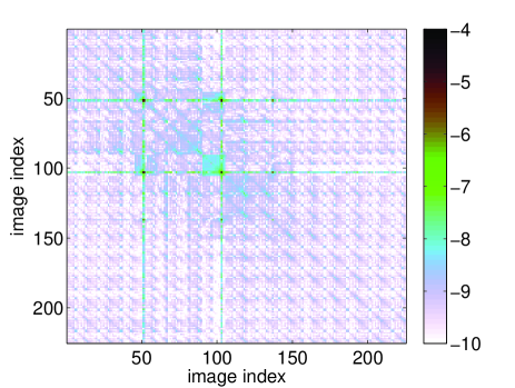
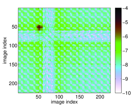
Figure 4: ($a$) The logarithm (base 10) of the image covariance matrix due to calibration errors and ($b$) due to the measurement noise on the same color scale. The former is almost everywhere two orders of magnitude lower.

We compare the image covariance due to calibration errors to the image covariance due to the noise on the data in a simulation. The calibration parameters are calculated from a separate data set with the same data model and integration time. We computed the CRB for the $8\times 8$ URA using the relations presented in Section IV-A for the simultaneous solution of the omni-directional complex gains, $\mathbf{G}$, and the system noise power, $\sigma_{n}^{2}$, which was assumed to be the same for all array elements, assuming a short term integration over $N=16384$ samples. This CRB was used in (60) to compute the image covariance matrix due to calibration errors. The magnitudes of the matrix entries are shown in Fig. 4($a$), in a log scale.

The image covariance matrix due to the noise in the measurement was calculated using (LABEL:eq:covnoise) and is shown in Fig. 4($b$). This shows that the covariance of the image values due to the calibration errors is more concentrated at the source locations than the covariance due to the system noise, but is generally more than two orders of magnitude lower. These results indicate that the calibration errors only represent a minor contribution to the total effective noise, even when the calibration measurements are done on the same (short) time scales using sources of the same strength, i.e. when the calibration measurement is similar to the actual measurement.

V-B Calibration observations vs. self calibration

In the previous section we discussed the situation in which the array is calibrated in a separate measurement. This scheme requires an extremely stable instrument. In most practical applications, the calibration is therefore done on the same data that is also used to provide the final image (self calibration). It is interesting to see how these scenarios compare. To this end, we used the relationships presented in Section IV-A to compute the CRB for simultaneous estimation of the omni-directional complex gains, the apparent source powers, the source locations and the system noise power for the $8\times 8$ URA.

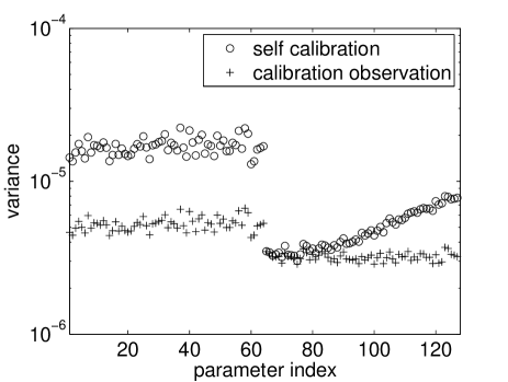
Figure 5: The CRB for the omni-directional complex gain amplitudes (parameters 1 through 64) and phases (parameters 65 through 127) for a separate calibration observation and the self calibration approach.

Figure 5 compares the CRBs for these two cases. The expected covariance of the gains and phases in the self calibration experiment is higher since more parameters have to be estimated simultaneously. The behavior of the CRB on the phases in the self calibrated observation (sloped upwards for increasing parameter index) can be explained by the interaction between the source parameters and the gain phases combined with the choice of the phase reference element in the corner of the array.

TABLE I: Covariance of source power estimates.

self calibration
index	2	3	4
2	$0.266\times 10^{-4}$	$0.287\times 10^{-4}$	$0.022\times 10^{-4}$
3	$0.287\times 10^{-4}$	$1.237\times 10^{-4}$	$0.048\times 10^{-4}$
4	$0.022\times 10^{-4}$	$0.048\times 10^{-4}$	$0.007\times 10^{-4}$
separate calibration
index	2	3	4
2	$0.280\times 10^{-4}$	$0.072\times 10^{-4}$	$0.006\times 10^{-4}$
3	$0.072\times 10^{-4}$	$0.772\times 10^{-4}$	$0.012\times 10^{-4}$
4	$0.006\times 10^{-4}$	$0.012\times 10^{-4}$	$0.005\times 10^{-4}$

Table I shows, for each of the two cases, the covariance matrices of the apparent source powers, i.e., the variance of the image values at the locations of the sources. The scaling factor ambiguity between $\mathbf{G}$ and $\Sigma$ in the self calibration case is resolved by putting $\sigma_{1}^{2}=1$ to constrain the problem, and therefore only the covariance values of the other three sources is tabulated. For the case with a separate calibration observation the covariance matrix was extracted from the sum of the image covariances due to calibration errors and system noise. The results in the table indicate that the variance of the source power estimates in both cases are comparable, although the source power estimates are slightly better when gain calibration data is available from a separate measurement. The covariance values found for a separate calibration stage are much lower than the corresponding values for self calibration. This suggests that pure imaging is more capable of separating source signals from different directions than self calibrated imaging.

VI Conclusions

In this paper we presented an analytic solution for snapshot imaging including deconvolution based on a data model (measurement equation) for the antenna signal covariance matrix or visibilities. The presented comprehensive framework is sufficiently flexible to enable extension of this analysis to synthesis observations, since the data model for a synthesis observation has the same form [11, 12, 13]. This framework allowed us to make the first complete rigorous assessment of the effective noise floor, which is the combined effect of propagated calibration errors, thermal noise and source confusion, in the image in terms of the covariance of the image values. Our simulations for a 2D uniform rectangular array indicate that the effect of propagated calibration errors is strongly concentrated at the source locations but is considerably smaller than the thermal noise at other image points. The results also suggest that if the instrument is sufficiently stable, a separate calibration step is to be preferred over a self calibrated image since it allows better source separation in the imaging process.

The effects of deconvolution can be described by a deconvolution matrix that describes the amount of linear independence (orthogonality) of the spatial signature vectors weighted by the actual gains of the receiving elements. A diagonal deconvolution matrix not only ensures the best possible spatial separation between the sources, but also ensures a homogeneous noise distribution over the map. This poses the question whether this matrix can be diagonalized by array design or by applying appropriate weights to the array elements. Since this factor is related to the array beam pattern, the latter is equivalent to finding weights that suppress the side lobe patterns at least in the direction of other sources, which suggest that techniques like Robust Capon Beamforming should provide the requested weighting [25]. The condition number of the deconvolution matrix can be used to assess the quality of the solution to the deconvolution problem.

Compared to a redundant array (ULA, URA), an array without redundant element spacings provides much better possibilities to approach the maximum number of solvable image points for a fixed number of antenna elements, thereby allowing the system to reach the theoretical self calibration confusion limit.

Stefan J. Wijnholds (S’2006) was born in The Netherlands in 1978. He received M.Sc. degrees in Astronomy and Applied Physics (both cum laude) from the University of Groningen in 2003. After his graduation he joined R&D department of ASTRON, the Netherlands Foundation for Research in Astronomy, in Dwingeloo, The Netherlands, where he works with the system design and integration group on the development of the next generation of radio telescopes. Since 2006 he is also with the Delft University of Technology, Delft, The Netherlands, where he is pursuing a Ph.D. degree. His research interests lie in the area of array signal processing, specifically calibration and imaging.

Alle-Jan van der Veen (F’2005) was born in The Netherlands in 1966. He received the Ph.D. degree (cum laude) from TU Delft in 1993. Throughout 1994, he was a postdoctoral scholar at Stanford University. At present, he is a Full Professor in Signal Processing at TU Delft. He is the recipient of a 1994 and a 1997 IEEE Signal Processing Society (SPS) Young Author paper award, and was an Associate Editor for IEEE Tr. Signal Processing (1998–2001), chairman of IEEE SPS Signal Processing for Communications Technical Committee (2002-2004), and Editor-in-Chief of IEEE Signal Processing Letters (2002-2005). He currently is Editor-in-Chief of IEEE Transactions on Signal Processing, and member-at-large of the Board of Governors of IEEE SPS. His research interests are in the general area of system theory applied to signal processing, and in particular algebraic methods for array signal processing, with applications to wireless communications and radio astronomy.

References

- [1] J. D. Bregman, “LOFAR Approaching the Critical Design Review,” in Proceedings of the XXVIIIth General Assembly of the International Union of Radio Science (URSI GA), New Delhi, India, Oct. 23-29 2005.
- [2] P. Hall, “The Square Kilometer Array: an International Engineering Perspective,” Experimental Astronomy, vol. 17, no. 1, pp. 5–16, 2004.
- [3] C. J. Lonsdale, R. J. Cappello, J. E. Salah, J. N. Hewitt, M. F. Morales, L. J. Greenhill, R. Webster and D. Barnes, “The Mileura Widefield Array,” in Proceedings of the XXVIIIth General Assembly of the Internatio nal Union of Radio Science (URSI GA), New Delhi, India, Oct. 23-29, 2005.
- [4] T. J. Cornwell, K. Golap and S. Bhatnagar, “-projection: A New Algorithm for Wide Field Imaging with Radio Synthesis Arrays,” in ADASS XIV, ser. Astronomical Society of the Pacific Conference Series, vol. 347, 2005.
- [5] R. A. Perley, “Wide Field Imaging II: Imaging with Non-coplanar Arrays,” in Synthesis Imaging in Radio Astronomy, ser. Astronomical Society of the Pacific Conference Series, Richard A. Perley, Frederic R. Schwab, Alan H. Bridle, Ed., vol. 6, 1994, pp. 139–165.
- [6] T. Cornwell, R. Braun and D. S. Briggs, “Deconvolution,” in Synthesis Imaging in Radio Astronomy II, ser. Astronomical Society of the Pacific Conference Series, G. B. Taylor, C. L. Carilli and R. A. Perley, Ed., vol. 180, 1999, pp. 151–170.
- [7] U. Schwarz, “Mathematical-statistical Description of the Iterative Beam Removing Technique (Method CLEAN),” Astronomy & Astrophyics, vol. 65, pp. 345–356, 1978.
- [8] S. Tan, “An Analysis of the Properties of CLEAN and Smoothness Stabilized CLEAN—Some Warnings,” Monthly Notices of the Royal Astronomical Society, vol. 220, pp. 971–1001, 1986.
- [9] S. R. Kulkarni, “Self-Noise in Interferometers: Radio and Infrared,” Astronomical Journal, vol. 98, no. 3, pp. 1112–1130, Sept. 1989.
- [10] S. J. Wijnholds, “Self-noise in full sky LOFAR images,” in Nederlandse Astronomen Conferentie (NAC), Ameland, The Netherlands, 10-12 May 2006.
- [11] A. Leshem and A. van der Veen, “Radio astronomical imaging in the presence of strong radio interference,” IEEE Tr. Information Th., vol. 46, no. 5, pp. 1730–1747, Aug. 2000. [Online]. Available: ftp://cas.et.tudelft.nl/pub/allejan-docs/it99.ps.gz
- [12] A.-J. van der Veen, A. Leshem and A.-J. Boonstra, “Array Signal Processing for Radio Astronomy,” Experimental Astronomy, vol. 17, no. 1-3, pp. 231–249, 2004.
- [13] S. van der Tol, B. Jeffs, and A. van der Veen, “Self calibration for the LOFAR radio astronomical array,” IEEE Tr. Signal Processing, vol. 55, no. 9, pp. 4497–4510, Sept. 2007. [Online]. Available: http://ens.ewi.tudelft.nl/pubs/jeffs06tsp.pdf
- [14] R. Narayan and R. Nityananda, “Maximum Entropy Image Restoration in Astronomy,” Annual Review of Astronomy & Astrophysics, no. 24, pp. 127–170, 1986.
- [15] R. O. Schmidt, “Multiple Emitter Location and Signal Parameter Estimation,” IEEE Trams. Antennas and Propagation, vol. AP-34, no. 3, Mar. 1986.
- [16] M. Viberg and B. Ottersten, “Sensor Array Processing Based on Subspace Fitting,” IEEE Trans. Signal Processing, vol. 39, no. 5, pp. 1110–1121, May 1991.
- [17] M. Viberg, B. Ottersten and T. Kailath, “Detection and Estimation in Sensor Arrays Using Weighted Subsp ace Fitting,” IEEE Trans. Signal Processing, vol. 39, no. 11, pp. 2436–2448, Nov. 1991.
- [18] M. Zatman, “How narrow is narrowband,” IEE Proc. Radar, Sonar and Navig., vol. 145, no. 2, pp. 85–91, Apr. 1998.
- [19] S. J. Wijnholds and A.-J. Boonstra, “A Multisource Calibration Method for Phased Array Radio Telescopes,” in 4th IEEE workshop on Sensor Array and Multichannel Processing (SAM), Waltham (MA), USA, 12-14July 2006.
- [20] S. J. Wijnholds, “Reducing the impact of station level spatial filtering limitations,” in SKA Calibration & Imaging Workshop (calim), Cape Town, South Africa, 4-6 Dec. 2006.
- [21] A. Thompson, J. Moran, and G. Swenson, Interferometry and Synthesis in Radio Astronomy, 2nd ed. John Wiley & Sons, Inc., 2001.
- [22] B. Ottersten, P. Stoica and R. Roy, “Covariance Matching Estimation Techniques for Array Signal Processing Applications,” Digital Signal Processing, A Review Journal, vol. 8, pp. 185–210, July 1998.
- [23] G. Golub and C. van Loan, Matrix Computations. Baltimore, MD: Johns Hopkins University Press, 1984.
- [24] T. K. Moon and W. C. Stirling, Mathematical Methods and Algorithms for Signal Processing. Upper Saddle River, New Jersey: Prentice Hall, 2000.
- [25] S. van der Tol and A. J. van der Veen, “Application of Robust Capon Beamforming to Radio Astronomical Imaging,” in IEEE Int. Conf. on Acoustics, Speech and Signal Proc. (ICASSP), Philadelphia (PA), Mar. 2005.
- [26] T. Cornwell and E. B. Fomalont, “Self-Calibration,” in Synthesis Imaging in Radio Astronomy, ser. Astronomical Society of the Pacific Conference Series, R. A. Perley, F. .R. Schwab and A. H. Bridle, Ed. BookCrafters Inc., 1994, vol. 6.
- [27] B. P. Flanagan and K. L. Bell, “Array Self-Calibration with Large Sensor Position Errors,” in IEEE Internatioal Conference on Acoustics, Speech and Signal Processing (ICASSP), 1999.
- [28] T. J. Pearson and A. C. S. Readhead, “Image Formation by Self-Calibration in Radio Astronomy,” Ann. Rev. Astron. Astrophys., vol. 22, pp. 97–130, 1984.
- [29] S. J. Wijnholds and A. J. van der Veen, “Effects of Parametric Constraints on the CRLB in Gain and Phase Estimation Problems,” IEEE Signal Processing Letters, vol. 13, no. 10, pp. 620–623, Oct. 2006.
- [30] S. Kay, Fundamentals of Statistical Signal Processing: Estimation Theory. Englewood Cliffs, New Jersey: Prentice Hall, 1993, vol. 1.
- [31] P. Stoica, B. Ottersten, M. Viberg, and R. Moses, “Maximum Likelihood Array Processing for Stochastic Coherent Sources,” IEEE Transactions on Signal Processing, vol. 44, no. 1, pp. 96–105, Jan. 1996.