Mach number dependence of electron heating
in high Mach number quasiperpendicular shocks

Abstract

Efficiency of electron heating through microinstabilities generated in the transition region of a quasi-perpendicular shock for wide range of Mach numbers is investigated by utilizing PIC (Particle-In-Cell) simulation and model analyses. In the model analyses saturation levels of effective electron temperature as a result of microinstabilities are estimated from an extended quasilinear (trapping) analysis for relatively low (high) Mach number shocks. Here, MTSI (modified two-stream instability) is assumed to become dominant in low Mach number regime, while BI (Buneman instability) to become dominant in high Mach number regime, respectively. It is revealed that Mach number dependence of the effective electron temperature in the MTSI dominant case is essentially different from that in the BI dominant case. The effective electron temperature through the MTSI does not depend much on the Mach number, although that through the BI increases with the Mach number as in the past studies. The results are confirmed to be consistent with the PIC simulations both in qualitative and quantitative levels. The model analyses predict that a critical Mach number above which steep rise of electron heating rate occurs may arise at the Mach number of a few tens.

I Introduction

Efficiency of electron heating in high Mach number collisionless shocks is one of the outstanding issues of space plasma physics as well as astrophysics. It is known from observations that quite efficient heating occurs in extremely high Mach number shocks like SNR (super nova remnant) shocks Park et al. (2006); Badenes et al. (2005, 2003); Hughes et al. (2000), while in-situ observations of earth’s bow shock mostly show inefficient heating of electrons Moses et al. (1985). This is probably due to the fact that a dominant electron heating process and its efficiency through a variety of microinstabilities in shock transition regions strongly depend on Mach numbers. Typical Mach number of the earth’s bow shock is $<10$, while that of the SNR shocks is of the order of $100-1000$. In the late 1980s a new process of strong and rapid electron heating in extremely high Mach number shocks was proposed Papadopoulos (1988); Cargil and Papadopoulos (1988). Refs. 6 and 7 discussed the so-called two step instabilities generated by a high velocity reflected ion beam which destabilizes BI (Buneman instability) followed by ion acoustic instability. A necessary condition for the BI to be destabilized in the foot of quasi-perpendicular shocks is $M_{A}/\sqrt{\beta_{e}}>20\sim 30$ Cargil and Papadopoulos (1988); Matsukiyo and Scholer (2003), where $M_{A}$ is the Alfvén Mach number and $\beta_{e}=8\pi nT_{e}/B^{2}$ the electron plasma beta. If the above condition is satisfied, rapid electron heating with saturation temperature $\propto M^{2}_{A}$ occurs and the ion acoustic instability sets in leading to further electron heating Papadopoulos (1988); Cargil and Papadopoulos (1988). This condition is easily satisfied in SNR shocks, although it is usually not in the earth’s bow shock.

The two step instabilities were again shed light on after Ref. 9 by utilizing electromagnetic full PIC (particle-in-cell) simulations. They improved understandings of the process not only in terms of electron heating but also in terms of a production process of non-thermal electrons, and promoted a number of subsequent simulation studies Hoshino and Shimada (2002); Shimada and Hoshino (2004); Dieckmann et al. (2004); Shimada and Hoshino (2005); McClements et al. (2005); Dieckmann et al. (2006); Amano and Hoshino (2007); Ohira and Takahara (2007, 2008); Umeda et al. (2008); Dieckmann and Bret (2009); Amano and Hoshino (2009a, b). As a result, understandings of electron heating or acceleration processes initiated by the BI in the context of the shock physics have been extensively developed.

On the other hand, it has been well-known that various microinstabilities are possible to get excited also in relatively low Mach number supercritical shocks Wu et al. (1984); Papadopoulos (1985). Since most of the microinstabilities are inseparable with electron dynamics, their nonlinear evolutions in self-consistently reproduced shock structures in PIC simulations are studied only recently (Scholer et al., 2003; Scholer and Matsukiyo, 2004; Muschietti and Lembege, 2006; Matsukiyo and Scholer, 2006a) except for Refs. 29-31. It is revealed that MTSI (modified two-stream instability) becomes dominant in the foot of the earth’s bow shock or interplanetary shocks at $\sim 1$ AU (Scholer et al., 2003; Scholer and Matsukiyo, 2004; Matsukiyo and Scholer, 2006a). Simulation studies on nonlinear evolutions of the MTSI in periodic systems were extensively studied in the 1970s and 1980s McBride et al. (1972); Ott et al. (1972); Tanaka and Papadopoulos (1983), although these simulations imposed some strong assumptions that the code was electrostatic McBride et al. (1972); Ott et al. (1972) and unmagnetized ions with small ion-to-electron mass ratio were used McBride et al. (1972); Ott et al. (1972); Tanaka and Papadopoulos (1983). Recently, some developement without these assumptions are made Matsukiyo and Scholer (2003, 2006b). Ref. 8 showed in a one-dimensional simulation with realistic mass ratio that long time evolution of the MTSI results in lower cascade of wave spectrum and associated electron heating. Furthermore, it is indicated in two-dimensional simulation that the MTSI can finally survive even if other possible instability like electron cyclotron drift instability is present Matsukiyo and Scholer (2006b). All these simulation studies show electron heating or acceleration in the long time evolution of the system. However, as mentioned already, electron heating in the earth’s bow shock is seldom observed in-situ.

Such a discripancy may arise because of lack of systematic estimate of electron heating rate in simulation studies with more realistic parameters. For example, all of the above simulation studies on the MTSI assume very low values of squared ratio of electron plasma to cyclotron frequencies, $\tau=\omega^{2}_{pe}/\Omega^{2}_{e}\leq 10$. Importance of $\tau$ in association with electron heating in the long time evolution of the MTSI is unresolved, while $\tau$ is known to be a crucial parameter controlling nonlinear electron heating and acceleration processes in the BI dominant system Shimada and Hoshino (2004). Electron plasma beta is also rather small in most of the previous studies ($\beta_{e}\leq 0.1$). This may exaggerate effects of electron trapping in the nonlinear stage of the MTSI McBride et al. (1972); Scholer et al. (2003); Matsukiyo and Scholer (2003); Scholer and Matsukiyo (2004); Matsukiyo and Scholer (2006a). The electron plasma beta in the solar wind is usually several times higher so that importance of the trapping process may be blurred. Hence, in realistic situations expected to be achieved in the typical solar wind conditions an alternative electron heating mechanism and its efficiency are ought to be considered.

In this paper, first, electron heating through the MTSI in transition regions of high Mach number quasi-perpendicular shocks is reconsidered in section II. Here, quasilinear diffusion is assumed as an alternative electron heating process. The analysis assumes a broad wave spectrum and small wave amplitudes which are likely to be satisfied in the past simulation studies mentioned above McBride et al. (1972); Matsukiyo and Scholer (2003). An additional assumption that relative phases among different wave modes are random is also imposed, while this point is currently not evident. Under these assumptions, taking second order velocity moments of the so-called quasilinear equations provides evolution equations of electron kinetic energies. These equations are numerically integrated by imposing the quasilinear assumptions in every instantaneous time steps to obtain saturation kinetic energies as a fuction of the Mach number of shocks. This approach allows to discuss long time evolution of macroscopic quantities including the electron temperature without any restrictions for parameters. It is intriguing whether the Mach number dependence of electron heating throug the MTSI in relatively low Mach number regime is different from that through the BI in extremely high Mach number regime. If that is the case, one may expect presence of a critical Mach number above which electron heating rate runs up due to the switching of the dominant microinstability Hoshino and Shimada (2002). In section III, the results are compared with 1D PIC simulations in which the MTSI is dominantly generated in the foot and effective electron temperature just behind of the shock is measured. Furthermore, post-shock effective electron temperature is measured also in cases that the BI gets excited in the foot. In those cases a rough estimate of the electron temperature is given by using the well-known trapping theory. Finally, a summary and discussions including estimate of the critical Mach number are given in section IV.

II Extended Quasilinear Analysis on Electron Heating through MTSI

II.1 System Configurations

A foot region of a quasiperpendicular shock is modeled by a plasma composed of incoming electrons at rest, incoming ions, and specularly reflected ions with local approximation. The ambient magnetic field is along the $z$-axis, while the incoming and the reflected ion beams are streaming parallel and antiparallel to a wavevector which is defined in the $x-z$ plane and parallel to the shock normal. This is essentially the same system discussed in the linear analysis of Ref. 8. Since the MTSI grows much faster than ion cyclotron period, ions are assumed to be unmagnetized.

II.2 Governing Equations

Saturation levels of electron kinetic energy through the MTSI are examined as follows. In a Vlasov equation,

$${\partial f_{j}\over\partial t}+{\bf v}\cdot\nabla f_{j}+{q_{j}\over m_{j}}\left({\bf E}+{{\bf v\times B}\over c}\right)\cdot\nabla_{\bf v}f_{j}=0,$$ (1)

variables are expanded around zero-th order slowly varying quantities (with subscript 0) as

$$\begin{array}[]{ccccc}f_{j}&=&F_{j0}&+&f_{j1},\\ {\bf B}&=&{\bf B_{0}}&+&{\bf B_{1}},\\ {\bf E}&=&&&{\bf E_{1}},\end{array}$$ (2)

where $f_{j}$, $q_{j}$, and $m_{j}$ are a distribution function, electric charge, and mass of species $j$, $c$ is speed of light, ${\bf B}$ and ${\bf E}$ represent magnetic and electric fields, respectively. The variables with subscript 1 denote fluctuations corresponding to linear oscillations. With a standard approach of quasilinear analysis, an evolution equation of $F_{j0}$ is obtained as follows Stix (1992); Kennel and Engelmann (1966).

$${\partial F_{0}\over\partial t}=\lim_{V\rightarrow\infty} {\pi q^{2}\over m^{2}}\sum^{\infty}_{n=-\infty}\int{d^{3}{\bf k}\over V}$$

$$Lv_{\perp}\delta(\omega_{r,{\bf k}}-k_{\parallel}v_{\parallel}-n\Omega)|\Psi_{n,{\bf k}}|^{2}v_{\perp}LF_{0}$$ (3)

Here, $V$ is the volume of integration, $\Omega=qB_{0}/mc$ the cyclotron frequency, $v_{\parallel}$ and $v_{\perp}$ the velocity components parallel and perpendicular to ${\bf B_{0}}$, ${\bf k}$ the wavevector which is also composed of parallel and perpendicular components $(k_{\parallel},k_{\perp})$, and $\omega_{r,{\bf k}}$ indicates real wave frequency which is a function of ${\bf k}$ and satisfies the linear dispersion relation. The subscript $j$ has been eliminated for simplicity. Only resonant wave-particle interactions corresponding to zero arguments of the delta function, $\omega_{r,{\bf k}}-k_{\parallel}v_{\parallel}-n\Omega=0\>(n=0,\pm 1,\pm 2,\cdots)$, are taken into account. Moreover,

$$L={1\over v_{\perp}}\left[\left(1-{k_{\parallel}v_{\parallel}\over\omega_{r}}\right){\partial\over\partial v_{\perp}}+{k_{\parallel}v_{\perp}\over\omega_{r}}{\partial\over\partial v_{\parallel}}\right],$$ (4)

$$|\Psi_{n,{\bf k}}|^{2}= {E^{2}_{1,{\bf k}}\over 1+A^{2}_{\perp}+A^{2}_{\parallel}}\left[{(1+A_{\perp})^{2}\over 4}J^{2}_{n-1}(\zeta)\right.$$

$$\left.+{(1-A_{\perp})^{2}\over 4}J^{2}_{n+1}(\zeta)+{v^{2}_{\parallel}\over v^{2}_{\perp}}A^{2}_{\parallel}J^{2}_{n}(\zeta)\right],$$ (5)

where $A_{\parallel}=E_{1z,{\bf k}}/E_{1x,{\bf k}},A_{\perp}=iE_{1y,{\bf k}}/E_{1x,{\bf k}}$, $E^{2}_{1,{\bf k}}=E^{2}_{1x,{\bf k}}+E^{2}_{1y,{\bf k}}+E^{2}_{1z,{\bf k}}$, and $J_{n}(\zeta)$ represents the $n-$th order Bessel function with argument $\zeta=k_{\perp}v_{\perp}/\Omega$. When the above expression of $\Psi_{n,{\bf k}}$ is derived, the linear dispersion relation is taken into account. Note that in eqs.(II.2)-(II.2) parallel and perpendicular directions are defined in terms of ${\bf B_{0}}$. Although this is true for electrons, further note is needed for ions. Because ions are assumed to be unmagnetized, distinction of parallel and perpendicular directions in this sense is meaningless. However, their evolution equations can be formally written in a similar form by defining parallel and perpendicular directions in terms of the ion beam velocity. This corresponds to a transformation for the rotation of the susceptibility tensor Matsukiyo and Scholer (2003).

To discuss the extended quasilinear evolution of kinetic energies through the MTSI, we examine parallel and perpendicular kinetic energy densities defined by

$$K_{\parallel}(t)={m\over 2}\int d^{3}{\bf v}(v_{\parallel}-v_{0})^{2}F_{0},$$ (6)

$$K_{\perp}(t)={m\over 2}\int d^{3}{\bf v}v^{2}_{\perp}F_{0}.$$ (7)

After some algebra, the following evolution equations of the kinetic energies are obtained.

$${\partial K_{\parallel}\over\partial t} =\lim_{V\rightarrow\infty}{2\pi^{2}q^{2}\over m}\sum_{n}\int{d^{3}{\bf k}\over V}\left[{\nu\over\omega_{r,{\bf k}}|k_{\parallel}|}\right.$$

$$\left.\left({n\Omega\over\omega_{r,{\bf k}}v^{2}_{t\perp}}+{\nu\over\omega_{r,{\bf k}}v^{2}_{t\parallel}}\right)\int dv_{\perp}v^{3}_{\perp}(|\Psi_{n}|^{2}F_{0})_{\delta=0}\right]$$ (8)

$${\partial K_{\perp}\over\partial t} =\lim_{V\rightarrow\infty}{2\pi^{2}q^{2}\over m}\sum_{n}\int{d^{3}{\bf k}\over V}\left[{n\Omega\over\omega_{r,{\bf k}}|k_{\parallel}|}\right.$$

$$\left.\left({n\Omega\over\omega_{r,{\bf k}}v^{2}_{t\perp}}+{\nu\over\omega_{r,{\bf k}}v^{2}_{t\parallel}}\right)\int dv_{\perp}v^{3}_{\perp}(|\Psi_{n}|^{2}F_{0})_{\delta=0}\right]$$ (9)

Here, $\nu\equiv\omega_{r,{\bf k}}-k_{\parallel}v_{0}-n\Omega$, and $()_{\delta=0}$ means a corresponding value at which the argument of the delta function is zero. The spectral energy density of the electric field fluctuations evolves as

$${\partial E^{2}_{\bf k}\over\partial t}=2\gamma_{\bf k}E^{2}_{\bf k},$$ (10)

where $\gamma_{\bf k}(t)$ denotes the linear growth rate of the wave mode having wavevector ${\bf k}$. Conservation of total energy is written as

$$\sum_{j}\left({n_{j}m_{j}\over 2}v^{2}_{j0}+K_{j\parallel}+K_{j\perp}\right)+\sum_{\bf k}{E^{2}_{1{\bf k}}\over 8\pi}=const.$$ (11)

Here, $n_{j}$ and $v_{j0}(t)$ denote density and bulk velocity of species $j$. Note that $\partial K_{\perp}/\partial t=0$ for unmagnetized ions and $v_{e0}=0$. Further, $\omega_{r,{\bf k}}$ and $\gamma_{\bf k}$ are defined at an instantaneous time. Eqs.(II.2)-(11) form a closed set of extended quasilinear evolution equations of the system. We solve the above set of equations numerically in the following subsection.

Similar analyses were performed by many authors McBride et al. (1972); Davidson and Ogden (1975); Ishihara and Hirose (1983a, b). Ref. 38 introduced detailed procedure of the method and applied it to estimate of saturation of electromagnetic ion cyclotron instability driven by ion temperature anisotropy. Refs. 39 and 40 directly solved the quasilinear equation to discuss electron heating and formation of a high energy ion tail through the ion acoustic instability. Ref. 33, on the other hand, discussed a problem similar to here on the MTSI and gave detailed comparisons of their results with 1d and 2d PIC simulations. However, their analysis includes only nonresonant wave-particle interactions which in turn only slight electron heating which is much less effective compared with a subsequent heating process through nonlinear trapping observed in their PIC simulation. Furthermore, they imposed an electrostatic assumption on whole their analyses as well as on their PIC simulations. As they pointed out, the electrostatic approximation is valid only when $v_{j0}/v_{A}<(1+\beta_{e})^{1/2}$, where $v_{A}$ denotes the Alfvén velocity, and $\beta_{e}$ is the electron plasma beta (ratio of electron thermal to magnetic pressures). Usually in solar wind $\beta_{e}$ is of the order of $0.1-1$ so that the above condition reads $v_{j0}/v_{A}\stackrel{{\scriptstyle<}}{{\sim}}1$ which is probably satisfied only in transition regions of rather low Mach number shocks. Since our attention is paid for wide range of Mach numbers, we exclude such an assumption.

Before solving eqs.(II.2)-(11) numerically, a few assumptions are imposed. The distribution functions of each species remain in (shifted) Maxwellian all the time after Ref. 38. By this assumption, it is easy to obtain $\omega_{r,{\bf k}}(t)$ and $\gamma_{\bf k}(t)$ at each time step as instantaneous solutions of the linear dispersion relation. The actual distribution functions are given by

$$F_{j0}={n_{j}\over(2\pi)^{3/2}v_{tj\parallel}v^{2}_{tj\perp}}\exp\left(-{(v_{j\parallel}-v_{j0})^{2}\over 2v^{2}_{tj\parallel}}-{v^{2}_{j\perp}\over 2v^{2}_{tj\perp}}\right)$$ (12)

for species $j$. Here $v_{tj\parallel}=\sqrt{T_{j\parallel}/m_{j}}$ and $v_{tj\perp}=\sqrt{T_{j\perp}/m_{j}}$ denote parallel and perpendicular thermal velocities. As mentioned before, note that the parallel and perpendicular directions are difined in association with ${\bf B_{0}}$ for electrons, while with ${\bf v_{j0}}$ for incoming and reflected ions. The bulk velocities of the incoming and reflected ions (subscripts $j=i$ and $r$, respectively) satisfy zero current condition so that $n_{i}v_{i0}+n_{r}v_{r0}=0$. It is also assumed that the response of the ions to the wave fields is electrostatic, while the wave-electron interactions are treated as fully electromagnetic. Therefore, the ion heating is thought to be parallel to ${\bf v_{i0}}$ or ${\bf v_{b0}}$.

Under these assumptions, we obtain the following evolution equations of kinetic energies.

$${\partial K_{e\parallel}\over\partial t} =\lim_{V\rightarrow\infty}{2\pi^{2}e^{2}\over m_{e}}\sum_{n}\int{d^{3}{\bf k}\over V}\left[{\nu_{e}\over\omega_{r,{\bf k}}|k_{\parallel}|}\right.$$

$$\left.\left({-n\Omega_{e}\over\omega_{r,{\bf k}}v^{2}_{te\perp}}+{\nu_{e}\over\omega_{r,{\bf k}}v^{2}_{te\parallel}}\right)\int dv_{\perp}v^{3}_{\perp}(|\Psi_{n}|^{2}F_{e0})_{\delta=0}\right]$$ (13)

$${\partial K_{e\perp}\over\partial t} =\lim_{V\rightarrow\infty}{2\pi^{2}e^{2}\over m_{e}}\sum_{n}\int{d^{3}{\bf k}\over V}\left[{-n\Omega_{e}\over\omega_{r,{\bf k}}|k_{\parallel}|}\right.$$

$$\left.\left({-n\Omega_{e}\over\omega_{r,{\bf k}}v^{2}_{te\perp}}+{\nu_{e}\over\omega_{r,{\bf k}}v^{2}_{te\parallel}}\right)\int dv_{\perp}v^{3}_{\perp}(|\Psi_{n}|^{2}F_{e0})_{\delta=0}\right]$$ (14)

$${\partial K_{i\parallel}\over\partial t}=\lim_{V\rightarrow\infty} {2\pi^{2}e^{2}\over m_{i}}\int{d^{3}{\bf k}\over V}\left[{1\over|k|}\left({\nu_{i}\over\omega_{r,{\bf k}}v_{ti\parallel}}\right)^{2}\right.$$

$$\left.\int dv_{\perp}v^{3}_{\perp}(|\Psi_{0}(z=0)|^{2}F_{i0})_{\delta=0}\right]$$ (15)

Here, $\nu_{e}=\omega_{r,{\bf k}}+n\Omega_{e}$ and $\nu_{i}=\omega_{r,{\bf k}}-kv_{i0}$, respectively. In this analysis only the linear resonant wave-praticle interactions are taken into account. Therefore, change of kinetic energy of the reflected ions ($K_{r\parallel}$) can be neglected when we consider the MTSI based on electron-incoming ion interactions. That is, here, the reflected ions are assumed to be a background component satisfying current and charge neutralities. Reactions of the reflected ions may be essential when influences of the MTSI on the reformation process are considered Scholer and Matsukiyo (2004). However, it is out of scope in this paper. In the following we solve eqs.(II.2)-(II.2), (10), and

$${n_{i}m_{i}\over 2}v^{2}_{i0}+K_{i\parallel}+K_{e\parallel}+K_{e\perp}+\sum_{\bf k}{E^{2}_{1{\bf k}}\over 8\pi}=const.$$ (16)

instead of eq.(11). Eq.(16) is actually used to determine $v^{2}_{i0}$. Note that contributions from the terms $|n|>4$ for $\sum_{n}$ in eqs.(II.2) and (II.2) are neglected. The validity of such an assumption will be checked in the following subsection.

II.3 Numerical Solutions

Figure 1: Time evolution of the system.

First, let us overview in Fig.1 time evolutions of the variables calculated in the system for a typical case. The initial parameters are $\mu\equiv m_{i}/m_{e}=1836,\tau\equiv\omega^{2}_{pe}/\Omega^{2}_{e}=10^{4},\beta\equiv 8\pi n_{e}(T_{e}+T_{i})/B^{2}_{0}\equiv\beta_{e}+\beta_{i}=0.4,\alpha\equiv n_{r}/n_{i}=1/3,\theta_{Bk}(=\Theta_{Bn})=85.5^{\circ}$, and $M_{A}\equiv(v_{i0}/v_{A})(1+\alpha)/2\alpha=6$. Here, the initial temperatures are isotropic and $\beta_{e}=\beta_{i}$. $M_{A}$ and $\alpha$ determine the initial $v_{i0}$ from the zero current condition. $\theta_{Bk}(\Theta_{Bn})$ denotes the angle between the ambient magnetic field, ${\bf B_{0}}$, and the wavevector (the shock normal), ${\bf k}({\bf n})$. The above parameters are fixed throughout the analysis if not specified. The field energy is given as appropriately small value: $E^{2}_{1}/B^{2}_{0}=10^{-10}$. For the moment, $kc/\omega_{pe}$ is fixed to unity just for simplicity. The field energy exponentially grows in the beginning of the run, although other variables have not been much changed in a visible manner until the field energy reaches at a certain level. Then $v_{i0}$ gradually decreases, while $K_{e\parallel}$ and $K_{i}$ increase ($\Omega_{i}t>0.2$). At the same time, the wave growth slows down and it starts damping after $\Omega_{i}t\sim 0.45$. Correspondingly, changing rates of other variables decrease and those variables approach some constant values when the field energy becomes sufficiently small. Such a state is regarded as a saturation state and those constant values are defined as saturation levels. The saturation state in this system is achieved when the field energy is damped out. In the analysis we check whether the system saturates basically by eye. However, in some special cases where the kinetic energies have not reached at constant values for long time the saturation levels are defined as the values at $t=t_{0}+2\Omega^{-1}_{i}$ where $t_{0}$ is the time at which $v_{i0}$ decreases by $1\%$ from its initial value. Since $2\Omega^{-1}_{i}$ is thought to be a typical time scale of shock reformation, considering the system evolution longer than this time scale may not make sense.

In Fig.1 $K_{e\perp}$ keeps almost constant incontrast to $K_{e\parallel}$ or $K_{i}$. This reflects which kinetic effects dominantly work. The linear growth rate, $\gamma_{k}$, can be written by linear superposition of the terms such as

$$-\xi_{j0}\exp(-\xi^{2}_{jn}),$$ (17)

where $\xi_{en}=(\omega_{r}+n\Omega_{e})/k_{\parallel}v_{te\parallel}$ and $\xi_{i0}=(\omega_{r}-kv_{i0})/kv_{ti}$, respectively. When $|\xi_{jn}|\sim 1$, contribution from the corresponding term to the growth rate becomes non-negligible. In this sense $\xi_{e0},\xi_{e1}$, and $\xi_{i0}$ can be indicators how strong the effects of Landau and cyclotron dampings of electrons, and inverse ion Landau damping are, respectively. The bottom panel of Fig.1 represents values of these indicators. It is now clear that the electron Landau damping is the strongest kinetic effect and the electron cyclotron damping hardly works. The inverse ion Landau damping can also work, but may not be so strong as the electron Landau damping for this particular case. This can explain the fact that increase of $K_{e\parallel}$ is most remarkable, while that of $K_{e\perp}$ is unrecognized. Contributions from other electron cyclotron harmonics ($\xi_{en}$ with $n=-1,\pm 2,\pm 3,\pm 4$) are further ineffective, and this is confirmed to be true for wide range of parameters (not shown). Therefore, effects of electron cyclotron interactions will be neglected in the remaining of the analysis. The assumption that $kc/\omega_{pe}=1$ is fixed is removed hereafter.

Figure 2: Saturation level of normalized parallel electron temperatures, $\beta_{e\parallel}$, as a function of (upper panel) initial $\beta_{0}$ and (lower panel) $\tau$. The three lines correspond to cases with different initial temperature ratio. The solid line with circles denotes the case with $\beta_{0e\parallel}/\beta_{0i}=1$, the dashed line with squares $\beta_{0e\parallel}/\beta_{0i}=3$, and the dotted line with triangles $\beta_{0e\parallel}/\beta_{0i}=1/3$, respectively.

The upper panel of Fig.2 denotes saturation levels of normalized electron temperature, $\beta_{e\parallel,sat}=8\pi n_{e}T_{e\parallel,sat}/B^{2}_{0}$ as a function of the initial $\beta_{0}=\beta_{0e}+\beta_{0i}$ when $\tau=10^{4}$. In calculating the right hand sides of eqs.(II.2)-(II.2), we chose interval of integration with respect to $k$ as $0\leq kc/\omega_{pe}\leq 3$ and grid size in $k$ as $\Delta kc/\omega_{pe}=0.06$. $\theta_{Bk}=85.5^{\circ}$ is again fixed here. In both upper and lower panels the solid line with circles, the dashed line with squares, and the dotted line with triangles correspond to the cases for $\beta_{0e\parallel}/\beta_{0i}=1,3$, and $1/3$, respectively. $\beta_{e\parallel,sat}$ is essentially independent from $\beta_{0}$ for $\beta_{0}>0.4$ indicating that heating process is similar for relatively high $\beta_{0}$. In the low $\beta_{0}$, on the other hand, there is a trend that electron heating is suppressed for $\beta_{0e\parallel}/\beta_{0i}=1/3$. For sufficiently low $\beta_{0e\parallel}$, number of resonant particles is very little so that it takes extremely long time to heat electrons. Then after the very long time, heating is suddenly triggered when field energy becomes large enough. Such an unnatural time evolution occurs because of the assumptions that only the resonant wave-particle interactions are taken into account and that the distribution functions are always Maxellian. Indeed, it is known from PIC simulations that effects of particle trapping, which have not been included in this analysis, become important for low $\beta_{0}$ cases Matsukiyo and Scholer (2003, 2006b). The initial electron to ion temperature ratio, $\beta_{0e\parallel}/\beta_{0i}$, affects the saturation levels. For large (small) $\beta_{0e\parallel}/\beta_{0i}(=3(1/3))$, $\beta_{e\parallel,sat}$ is high (low). Comparing with the case of $\beta_{0e\parallel}/\beta_{0i}=1$, $|\xi_{i0}|$ gets closer to unity because $v_{ti}$ gets larger when $\beta_{0e\parallel}/\beta_{0i}$ becomes 1/3. Hence, the inverse ion Landau damping works more effectively so that electron heating becomes less dominant. The $\tau$ dependence of $\beta_{e\parallel,sat}$ is shown in the lower panel of Fig.2 for $\beta_{0}=0.4$. As expected from the linear analysis Matsukiyo and Scholer (2003), dependence on $\tau$ is rather weak. This implies that using small $\tau$ in simulations does not lead to unrealisitic results for long time evolution of the MTSI.

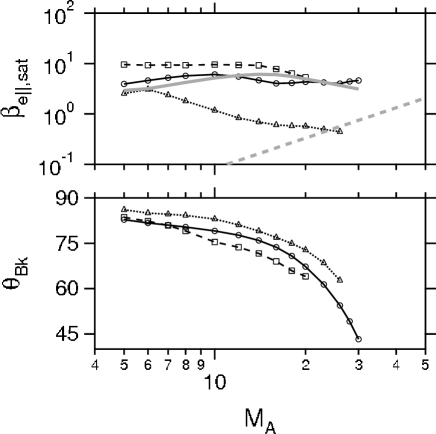
Figure 3: Mach number dependence of (upper panel) maximum saturation electron temperatures, $\beta_{e\parallel}$, and (lower panel) corresponding wave propagation angles, $\theta_{Bk}$. The three black lines correspond to cases with different initial temperature ratio. Their definition is given in the caption of Fig.2. The thick gray solid (dashed) line is obtained from eq.(18) (eq.(19)).

Fig.3 represents $M_{A}$ dependense for $\tau=10^{4}$ and $\beta_{0}=0.4$. Three black lines (the solid line with circle, the dashed line with squares, and the dotted line with triangles) in the upper panel denote the maximum saturation levels of $\beta_{e\parallel,sat}$ in varying $\theta_{Bk}$ again for different initial temperature ratios ($\beta_{0e\parallel}/\beta_{0i}=1,3,1/3$). The corresponding values of $\theta_{Bk}$ is indicated in the bottom panel. $\beta_{e\parallel,sat}$ does not increase so much, even though the $M_{A}$ gets larger. As already mentioned, the system saturates when available field energy is lost and no more waves grow. Such a state may be achieved when effect of electron Landau damping becomes efficient. If it is the case, $\eta\xi_{e0}\approx 1$ should be satisfied at the saturation state. Here $\eta$ is a factor of the order of unity and is empirically determined later. By using $v^{2}_{te\parallel}=T_{e\parallel}/m_{e}$ and $\omega/k_{\parallel}\approx v_{i0}/\cos\theta_{Bk}$,

$$\beta_{e\parallel,sat}\sim{2\eta^{2}M^{2}_{A}\over\mu\cos^{2}\theta_{Bk}}\left({2\alpha\over 1+\alpha}\right)^{2}.$$ (18)

The gray thick solid line in Fig.3 is obtained by substituting the values of $\theta_{Bk}$ of the solid line in the bottom panel into eq.(18). Here, $\eta=2.6$ has been assumed. Although dependence on initial tempetarure ratio, $\beta_{0e\parallel}/\beta_{0i}$, is not trivial in eq.(18), this may give a reasonable order of magnitude estimate. Remember that in the MTSI a cross-field ion beam interacts with oblique whistler waves. The whistler waves which can interact with the high speed ion beam should have appropriately high phase velocities. The phase velocity of an oblique whistler wave is proportional to $\cos\theta_{Bk}$ Matsukiyo and Scholer (2003) so that a high Mach number shock generates high phase velocity, i.e., less oblique, whistler waves. This effect appears in the bottom panel. As a result, $M_{A}/\cos\theta_{Bk}$ does not change so much even the Mach number varies, so that $\beta_{e\parallel,sat}$ remains in the same order for wide Mach number regime examined here. Only the dotted line with triangles in the upper panel is weakely decreasing function of the Mach number. In this relatively high initial ion temperature case, as mentioned earlier, ion kinetic effect seems to be non-negligible. As a result, ion heating is more remarkable than in the cases with $\beta_{0e\parallel}/\beta_{0i}=1,3$. Furthermore, because of small growth rate due also to the ion kinetic effect, it takes rather long time for the system to approach a final saturation state. Therefore, the saturation levels were actually estimated at $t=t_{0}+2\Omega^{-1}_{i}$ as mentioned before.

Note that the condition $\xi_{e0}\approx 1$ gives essentially same expression given in Ref. 33 which derives saturation energy due to electron trapping. Hence, the expression in eq.(18) may be applicable in also the low beta case for MTSI. However, because Ref. 33 assumed that $\mu\cos^{2}\theta_{Bk}$ is constant throughout their analyses, their saturation temperature increases with $M^{2}_{A}$. This might be true if the Mach number is sufficiently small and the electrostatic approximation is valid. But it is now clear that constant $\mu\cos^{2}\theta_{Bk}$ assumption is invalid at least for $M_{A}\geq 5$.

III Electron Heating Reproduced by 1D PIC Simulation

Table 1: Injection Plasma Parameters for Simulation

	$M_{Ain}$	$\tau$	$m_{i}/m_{e}$	$\beta_{e}$	$\beta_{i}$	$\theta_{Bn}$
Run A	4	16	625	0.3	0.1	84
Run B	6	16	625	0.3	0.1	81
Run C	10	16	625	0.3	0.1	79
Run D	8	100	64	0.3	0.1	90
Run E	16	100	64	0.3	0.1	90
Run F	30	100	64	0.3	0.1	90

Here, shock waves are actually reproduced by using one-dimensional PIC code and the resultant electron heating through MTSI and BI in the transition region is discussed. A shock is produced in the simulation domain by using the so-called reflecting wall method. An upstream plasma consisting of equal numbers of ions and electrons is continuously injected from the left-hand boundary ($x=0$) and carries a uniform magnetic field, ${\bf B_{0}}=(B_{0x},0,B_{0z})$, and a motional electric field, $E_{y}=u_{in}B_{0z}/c$, where $u_{in}$ is the injection flow velocity in the positive $x$-direction. At the right-hand boundary the particles are reflected. As a result of the interaction between the incoming and reflected particles a shock wave is produced and propagates in the negative $x$-direction. Thus the simulation frame is the downstream rest frame. The grid size is set to be $\Delta x\approx 0.83\lambda_{De}$ and 200 particles/cell are distributed for both ions and electrons at the injection boundary, where $\lambda_{De}$ denotes the electron Debye length. Physical parameters are summarized in TABLE 1. For runs A, B, and C (D, E, and F), MTSI (BI) gets excited in the foot during each reformation cycle.

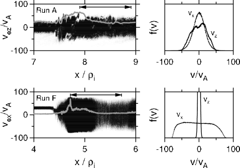
Figure 4: Electron heating observed in one dimensional PIC simulations for (upper panels) Run A and (lower panels) Run F. The left panels show electron phase space distributions in (upper left panel) $v_{ez}-x$ and (lower left panel) $v_{ex}-x$. The gray solid lines denote profiles of magnetic field $B_{z}$ component. The right panels indicate electron distribution functions in $v_{ex}$ and $v_{ez}$ integrated over space corresponding to the arrowed regions in the left panels.

Fig.4 shows two examples of snap shots of electron phase space $v_{z}-x$ at $\Omega_{i}t=6.02$ for Run A (upper left panel) and $v_{x}-x$ at $\Omega_{i}t=8.67$ for Run F (lower left panel). The gray solid lines denote profiles of magnetic field $B_{z}$ component. In both runs velocity distribution functions corresponding to the downstream areas indicated by arrows in the left panels are represented in the right panels. Nonadiabatic electron heating downstream of the shock is clearly observed. Parallel heating is superior to the adiabatic perpendicular heating in Run A, while strong perpendicular heating, or heating parallel to the beam velocity, is seen in Run F. The effective temperatures, $K^{eff}$, just downstream of the shocks are estimated by using the same definition as eqs.(6) and (7). We averaged over the particles distributed in the region of $x_{os}\leq x\leq x_{os}+\rho_{i}$, where $x_{os}$ is the position of the magnetic overshoot and $\rho_{i}$ the ion cyclotron radius defined by upstream flow velocity and ion cyclotron frequency. Because of nonstationarity of the shock, $K^{eff}$ is not constant in time. Therefore, $K^{eff}$ is also averaged in time a few shock reformation periods. The results are plotted in Fig.5 as a function of the injection Mach number, $M_{Ain}$. Here, $K^{eff}$ is normalized to the upstream magnetic pressure, $B^{2}_{01}/8\pi$, and rewritten as $\beta^{eff}$. For Runs A, B, and C, $\beta^{eff}_{e\parallel}$ is almost independent on $M_{Ain}$, which is consistent with the extended quasilinear analysis shown in the previous section. The dashed line just below the points A to C is drawn by using eq.(18) with assuming $\alpha=1/3$, $\eta=1$, and $M_{A}=M_{Ain}$.

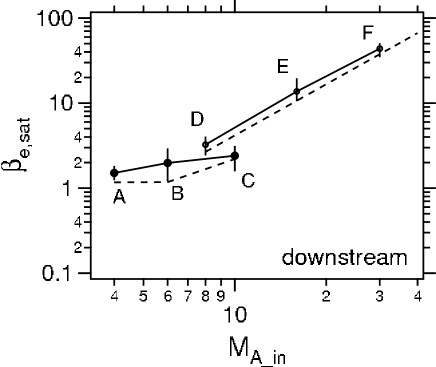
Figure 5: Comparison of normalized electron temperatures between the PIC simulations and the model analyses. The markers labeled A $\sim$ F are estimated as averaged effective electron temperatures downstream of the shocks reproduced in the PIC simulations. The dashed lines are obtained from the model analyses, eq.(18) for A $\sim$ C and eq(19) for D $\sim$ F, respectively.

On the other hand, $\beta^{eff}_{ex}$ efficiently increases with $M_{Ain}$ for Runs D, E, and F, where BI gets excited in the foot. Nonlinear development of the BI was well studied in the past. Especially, Ref. 10 analyzed it in detail by performing one dimensional PIC simulations with periodic boundary conditions modeling a part of the foot region in a perpendicular shock geometry. They showed that when $\tau\gg 1$, the BI produces well defined electron holes in its early nonlinear stage and some additional heating or acceleration occurs in the course of further long time evolution. Although a saturation level of the instability is reduced a little in two dimensional system, electron trapping still plays an important role through oblique modes Amano and Hoshino (2009b). It is infered from these results that size of the electron holes in phase space may give a lower limit of $\beta^{eff}_{ex}$. The amplitude of an electron hole was estimated by assuming that electrostatic wave energy density is comparable with drift energy density of electrons in the ion’s rest frame Ishihara et al. (1981); Hoshino and Shimada (2002). For our case, it reads

$$\beta^{eff}_{ex}\sim{8\over 1+\alpha}{M^{2}_{A}\over\mu^{7/6}},$$ (19)

where we assume the BI based on electron-reflected ion interactions which usually grows faster than the BI based on electron-incoming ion interactions so that $\Delta u/v_{A}=2M_{A}/(1+\alpha)$ is used as the relative drift velocity. As seen in the above expression, $\beta^{eff}_{ex}$ increases with $M^{2}_{A}$ which is proportional to the system free energy. This functional dependence is also derived in Refs. 6, 7, and 11. One can confirm that eq.(19) may give a good estimate of the lower limit of $\beta^{eff}_{ex}$ by plotting the corresponding values in Fig.5 for $\alpha=0.5$ and $\mu=64$ as the dashed line just below the points D to F. One should note that $M_{A}$ in eq.(19) is not necessarily coincide with $M_{Ain}$ in Fig.5. Because the $M_{A}$ indicates the local Mach number of the foot in the shock rest frame, while the $M_{Ain}$ denotes the injection Mach number in the simulation frame, i.e., the downstream rest frame. It is also hard to define the local Mach number of the foot from the simulation data, since the shock is not time stationary. Therefore, the dashed line should be regarded only as a guide.

IV Discussions

In the previous section it was confirmed that the extended quasilinear analysis for the MTSI and the trapping analysis for the BI give consistent results with the PIC simulations. Here, let us compare the results of these two analysis. The thick gray dashed line in Fig.3 denotes $\beta^{eff}_{ex}$ obtained from eq.(19) for $\mu=1836,\alpha=0.5$. This line intersects at $M_{A}\sim 24$ with the dotted line with triangles which is $\beta_{e\parallel,sat}$ for the MTSI with $\beta_{0e\parallel}/\beta_{0i}=1/3$. The gray thick solid line based on eq.(18) likely to intersect with the gray thick dashed line at $M_{A}\sim 45$. Depending on parameters, an actual intersection may occur in the range of $20<M_{A}<50$. If this is written as $M^{*}_{A}$, the dominant electron heating process possibly switches from the MTSI for $M_{A}<M^{*}_{A}$ to the BI for $M_{A}>M^{*}_{A}$. For relatively low Mach numbers like in the earth’s bow shock, $\beta_{e\parallel,sat}$ is more or less constant with $10^{0\sim 1}$ because the MTSI becomes dominant. If $\beta_{e,sat}=5$ and $\tau=10^{4}$ are assumed, corresponding electron temperature is $\sim 100$eV which is consistent with a typical temperature observed downstream of the earth’s bow shock. However, addiabatic heating due to increases of magnetic field and cross shock potential also results in the downstream electron temperature similar to this value. This may be the reason why remarkable electron heating was seldom observed in near earth shocks in the past. But one may capture the nonadiabatic parallel electron heating if upstream electron beta is low enough ($\beta_{e0}<0.1$), since eq.(18) is still valid for rather low beta cases where the trapping effects become essential as mentioned in section II. Furthermore, as shown in the upper right panel of Fig.4, local temperature anisotropy, $T_{e\parallel}/T_{e\perp}>1$, in a transition region may be observed as a result of strong MTSI in some parameter regimes. On the other hand, the effective electron temperature significantly increases with being proportinal to $M^{2}_{A}$ in $M_{A}>M^{*}_{A}$. Although this is consistent with the past studies Papadopoulos (1988); Cargil and Papadopoulos (1988); Shimada and Hoshino (2005), the saturation electron temperature estimated in this study seems to be rather smaller. This should be because of that the heating process in highly nonlinear stage including the second step ion acoustic instability is neglected. Electron temperature seen in Ref. 10 seems to be about one order higher than the estimate given by eq.(19). This implies that an actual $M^{*}_{A}$ may appear at a little smaller value.

Consistency of the results of the extended quasilinear analysis and the PIC simulations for the MTSI dominant cases indicates that the resonant wave-particle interactions are essential in electron heating through the MTSI. In other wards, nonresonant wave-particle interactions which have been neglected in the analysis may not be effective. It should also be noted that using unrealistically small $\tau$ in PIC simulations is justified as far as the MTSI is concerned because of the weak dependence on $\tau$ (bottom panel of Fig.2) in contrast to the BI dominant systems.

The transition at $M_{A}=M^{*}_{A}$ might not be so drastic in a realistic case. In the analyses presented here, all other possible candidates of microinstabilities have been neglected. For example, ECDI (electron cyclotron drift instability) is one candidate Muschietti and Lembege (2006) and it might become important around this critical Mach number, although there are some negative indications for the ECDI to become dominant. For instance, it is known that the saturation level of the ECDI is usually not so high Wu et al. (1984). In addition, if the ECDI gets excited simultaneously with the MTSI, the MTSI becomes dominant for wide parameter range Matsukiyo and Scholer (2006b). Furthermore, it is shown that the ECDI can be important only when $\tau$ is of the order of unity Shimada and Hoshino (2004). Hence, the Mach number regime where the ECDI is dominant seems not to be so wide, but we do not remove the possibility that the ECDI gives some contributions to electron heating around $M^{*}_{A}$. Because the ECDI is insensitive to the electron Landau damping which may strongly affect to the BI in this Mach number regime. Further, it is known that the MTSI cannot get excited in extremely high Mach number shocks like $M_{A}>30\sim 40$ Matsukiyo and Scholer (2003). There are also other possible microinstabilities in higher dimensional cases Wu et al. (1984). Contributions from them should be carefully estimated. Some of them have been discussed recently by performing two dimensional PIC simulations Ohira and Takahara (2008); Umeda et al. (2008); Amano and Hoshino (2009a). The multi-dimansionality may give another important contributions to electron heating. Ref. 42 pointed out that electrons are accelerated in the so-called rippled structure which is the ion scale structure along the shock surface. Nevertheless, what should be emphasized here is that the Mach number dependence of the effective electron temperature is systematically different between high and low Mach number regimes.

In the present extended quasilinear analysis the damping of the wave energy in the late stage (e.g., $\Omega_{i}t>0.45$ in Fig.1) may be an artifact. Because of the assumption that the distribution function is always Maxwellian, the so-called plateau of the distribution function is never produced in this system. The field energy might saturate earlier at a certain level if the plateau is produced. In this regard, it might be better that the saturation levels are defined as the values at the time when the field energy becomes the maximum. However, the resultant saturation levels based on the two definitions, i.e., the saturation temperatures estimated at times corresponding to the maximum and the later sufficiently small field energies, are not so much different from each other. Although it is possible to solve the quasilinear equation, eq.(II.2), directly as done in Refs. 39 and 40, that is the future work.

The explorations of the inner heliosphere will be underway through the BepiColombo mission. The perihelion point of the mercury is about 0.3AU where quite high velocity IPSs which have not been decerelated are expected to be observed. Ref. 43 estimated the propagation speed of one of the IPSs observed in August 1972 and concluded that it approached to $\sim 2000$ km/s at 0.3AU from the sun. More optimistic estimate for the same IPS is given in Ref. 44 as $\sim 4000$ km/s at 0.3AU. These results imply that the Mach number of this IPS approached to several tens. Therefore, the transition of the electron heating efficiency at $M^{*}_{A}$, if present, will be possibly observed in situ Hoshino and Shimada (2002).

References

- Park et al. (2006) S. Park, S. A. Zhekov, D. N. Burrows, P. G. Garmire, J. L. Racusin, and R. McCray, Astrophys. J. 646, 1001 (2006)
- Badenes et al. (2003) C. Badenes, E. Bravo, K. J. Borkowski, and I. Domínguez, Astrophys. J. 593, 358 (2003)
- Badenes et al. (2005) C. Badenes, K. J. Borkowski, and E. Bravo, Astrophys. J. 624, 198 (2005)
- Hughes et al. (2000) J. P. Hughes, C. E. Rakowski, and A. Decourchelle, Astrophys. J. 543, L61 (2000)
- Moses et al. (1985) S. L. Moses, F. V. Coroniti, C. F. Kennel, and F. L. Scarf, Geophys. Res. Lett. 12, 609 (1985)
- Papadopoulos (1988) K. Papadopoulos, Astrophys. Space Sci. 144, 535 (1988)
- Cargil and Papadopoulos (1988) P. J. Cargill and K. Papadopoulos, Astrophys. J. 329, L29 (1988)
- Matsukiyo and Scholer (2003) S. Matsukiyo and M. Scholer, J. Geophys. Res. 108, SMP19-1, 1459 (2003)
- Shimada and Hoshino (2000) N. Shimada and M. Hoshino, Astrophys. J. 543, L67 (2000)
- Shimada and Hoshino (2004) N. Shimada and M. Hoshino, Phys. Plasmas 11, 1840 (2004)
- Shimada and Hoshino (2005) N. Shimada and M. Hoshino, J. Geophys. Res. 110, A02105 (2005)
- Hoshino and Shimada (2002) M. Hoshino and N. Shimada, Astrophys. J. 572, 880 (2002)
- Dieckmann et al. (2004) M. E. Dieckmann, B. Eliasson, P. K. Shukla, Astrophys. J. 617, 1361 (2004)
- Dieckmann et al. (2006) M. E. Dieckmann, B. Eliasson, M. Parviainen, P. K. Shukla, A. Ynnerman, Mon. Not. R. Astron. Soc. 367, 865 (2005)
- McClements et al. (2005) K. G. McClements, R. O. Dendy, M. E. Dieckmann, A. Ynnerman, and S. C. Chapman, J. Plasma Phys. 71, 127 (2005)
- Ohira and Takahara (2007) Y. Ohira and F. Takahara, Astrophys. J. 661, L171 (2007)
- Ohira and Takahara (2008) Y. Ohira and F. Takahara, Astrophys. J. 688, 320 (2008)
- Amano and Hoshino (2007) T. Amano and M. Hoshino, Astrophys. J. 661, 190 (2007)
- Amano and Hoshino (2009a) T. Amano and M. Hoshino, Astrophys. J. 690, 244 (2009)
- Amano and Hoshino (2009b) T. Amano and M. Hoshino, Phys. Plasmas 16, 102901 (2009)
- Umeda et al. (2008) T. Umeda, M. Yamao, and R. Yamazaki, Astrophys. J. 681, L85 (2008)
- Dieckmann and Bret (2009) M. E. Dieckmann and A. Bret, Astrophys. J. 694, 154 (2009)
- Papadopoulos (1985) K. Papadopoulos, AGU Geophys. Mon. 34, 59 (1985)
- Wu et al. (1984) C. S. Wu, D. Winske, Y. M. Zhou, S. T. Tsai, P. Rodriguez, M. Tanaka, K. Papadopoulos, K. Akimoto, C. S. Lin, M. M. Leroy, and C. C. Goodrich, Space Sci. Rev. 37, 63 (1984)
- Scholer et al. (2003) M. Scholer, I. Shinohara, and S. Matsukiyo, J. Geophys. Res. 108, SSH4-1, 1014 (2003)
- Scholer and Matsukiyo (2004) M. Scholer and S. Matsukiyo, Ann. Geophys. 22, 2345 (2004)
- Matsukiyo and Scholer (2006a) S. Matsukiyo and M. Scholer, Adv. Space Res. 38, 57 (2006a)
- Muschietti and Lembege (2006) Muschietti, L. and Lembége, B., Adv. Space Res., 37, 483 (2006)
- Biskamp and Welter (1972a) D. Biskamp and H. Welter, Phys. Rev. Lett. 28, 410 (1972)
- Biskamp and Welter (1972b) D. Biskamp and H. Welter, Nucl. Fusion 12, 663 (1972)
- Biskamp and Welter (1972c) D. Biskamp and H. Welter, J. Geophys. Res. bf 77, 6052 (1972)
- Ott et al. (1972) E. Ott, J., B. McBride, J., H. Orens, and J., P. Boris, Phys. Rev. Lett. 28, 88 (1972)
- McBride et al. (1972) J., B. McBride, E. Ott, J., P. Boris, and J., H. Orens, Phys. Fluids 15, 2367 (1972)
- Tanaka and Papadopoulos (1983) M. Tanaka and K. Papadopoulos, Phys. Fluids 26, 1697 (1983)
- Matsukiyo and Scholer (2006b) S. Matsukiyo and M. Scholer, J. Geophys. Res. 111, L02101 (2006b)
- Kennel and Engelmann (1966) C. F. Kennel, and F. Engelmann, Phys. Fluids 9, 2377 (1966)
- Stix (1992) T. H. Stix, Waves in Plasmas, AIP, Chap.17 (1992)
- Davidson and Ogden (1975) R. C. Davidson and J. M. Ogden, Phys. Fluids 18, 1045 (1975)
- Ishihara and Hirose (1983a) O. Ishihara and A. Hirose, Phys. Rev. Lett. 50, 1783 (1983a)
- Ishihara and Hirose (1983b) O. Ishihara and A. Hirose, Phys. Fluids 26, 100 (1983b)
- Ishihara et al. (1981) O. Ishihara, A. Hirose, and A. B. Langdon, Phys. Fluids 24, 452 (1981)
- Burgess (2006) D. Burgess, Astrophys. J. 653, 316 (2006)
- Smart and Shea (1985) D. F. Smart and M. A. Shea, J. Geophys. Res. 90, 183 (1985)
- Dryer et al. (1975) M. Dryer, A. Eviatar, A. Frohlich, A. Jacobs, J. H. Joseph, and E. J. Weber, J. Geophys. Res. 80, 2001 (1975)