Improving chiral property of domain-wall fermions by reweighting method

Abstract:

The reweighting method is applied to improve the chiral property of domain-wall fermions. One way to achieve this is to enlarge $L_{s}$, the size of fifth dimension, which controls the size of the induced chiral symmetry breaking. While this is a type of reweighting method for shifting the action parameter, it seems non-trivial since this reweighting means change of the five dimensional lattice volume. In this report, we address issues in this direction of reweighting and evaluate its effectiveness.

RBRC-778

1 Introduction

The domain-wall (DW) fermion is one realization of the chiral fermion on the lattice [2, 3]. The DW fermion is constructed by five-dimensional formulation and has a parameter $L_{s}$, which is the size of fifth-dimension. The chiral symmetry is realized in the $L_{s}\rightarrow\infty$ limit. In realistic simulations, however, we have to take $L_{s}$ finite; then the symmetry is slightly broken. The broken chiral symmetry causes the additive mass shift $m_{res}$, which is called “residual mass” and captures the degree of the breaking. In recent lattice QCD simulations, we are going into the regime in which the quark mass is lighter and lighter and the volume is larger and larger. The computational resources required are becoming ever larger in these situations, and then it is hard to take $L_{s}$ so large that the chiral symmetry breaking is negligible. Improving the chiral property of the DW fermion is a natural thought in this circumstance. One possible strategy for this is introducing a twisted mass term to improve chiral symmetry, which suppresses a topology change  [4, 5]. Recently, reweighting techniques are becoming widely used in QCD simulations. Among them, the reweighting for the quark mass parameter is intensively applied and seems effective [6]. Our aim of this work is to enlarge $L_{s}$ by reweighting to improve the chiral property. In this report, we discuss some techniques toward the reweighting and its effectiveness. We also perform some simple tests as an experiment using $N_{f}=2+1$ dynamical DW fermion configurations with volume $L^{3}\times T\times L_{s}=16^{3}\times 32\times 8$:

Conf [A] $$: \beta=2.30~{}\mbox{(Iwasaki gluon)},~{}m_{ud}=0.04,~{}m_{s}=0.04,~{}M_{5}=1.8,$$ (1)

Conf [B] $$: \beta=2.13~{}\mbox{(Iwasaki gluon)},~{}m_{ud}=0.02,~{}m_{s}=0.04,~{}M_{5}=1.8,$$ (2)

produced by RBC and UKQCD Collaborations [7].

2 Reweighting factor

We consider to reweight configurations with $L_{s}=L_{1}$ to $L_{2}$ ($L_{1}<L_{2}$). In this work, we ignore the strange quark sector even though we use $N_{f}=2+1$ dynamical configurations because we assume the effect is small and the present work is at an experimental stage. The reweighting factor can be simply written by

$$w=\frac{\det\left[D_{2}^{\dagger}(m_{f})D_{2}(m_{f})\right]}{\det\left[D_{1}^{\dagger}(m_{f})D_{1}(m_{f})\right]}\frac{\det\left[D_{1}^{\dagger}(1)D_{1}(1)\right]}{\det\left[D_{2}^{\dagger}(1)D_{2}(1)\right]},$$ (3)

where $D_{i}(m_{f})$ represents DW Dirac matrix with parameter set $(L_{s}=L_{i},m_{f})$, where $m_{f}$ represents the bare DW fermion mass. One of the interesting features of this reweighting is the existence of the part with $m_{f}=1$ which is coming from Pauli-Villars (PV) field of the DW formalism. While the systems before and after the reweighting have different five-dimensional volume, the effect coming from the PV sector cancels out a large portion of the volume factor.

3 Stochastic estimation of the reweighting factor

In order to estimate the reweighting factor we use the stochastic estimator with random Gaussian noise. When we consider the determinant of a matrix $\Omega$, its stochastic estimation can be expressed by

$$\det\Omega=\frac{\int{\cal D}\xi e^{-\xi^{\dagger}\Omega^{-1}\xi}}{\int{\cal D}\xi e^{-\xi^{\dagger}\xi}}=\langle e^{-\xi^{\dagger}(\Omega^{-1}-1)\xi}\rangle_{\xi}=\langle e^{-H}\rangle_{\xi},$$ (4)

where $\langle\cdots\rangle_{\xi}$ denotes the ensemble average over complex random Gaussian noise vector $\xi$. A naive estimation, however, might end in failure. In this section, we explain several implementations used in the reweighting.

3.1 Canceling the fluctuations

A naive way to estimate the reweighting factor $w$  (3) is to calculate each determinant separately by using Eq. (4). This way, however, is not efficient, because each determinant can have large fluctuations. To reduce the large fluctuation, a determinant of the whole product of Dirac operators is estimated using one Gaussian noise $\xi$. For the efficient sampling of $e^{-H}$, we choose hermitian operator $\Omega=\phi^{\dagger}\phi$ in Eq. (4) and thus the reweighting factor becomes $w=\det\left[\phi^{\dagger}\phi\right]$. In this work, we take an operator for $\phi$ as

$$\phi={\cal D}_{2}(m_{f})\frac{1}{{\cal D}_{1}(m_{f})}{\cal D}_{1}(1)\frac{1}{{\cal D}_{2}(1)},$$ (5)

where a notation, ${\cal D}=\sqrt{D^{\dagger}D}$, is used, and the square root is implemented by the rational approximation  [8]. While we can, of course, write down the $\phi$ without using the square root, we use it on purpose for later convenience (See Sec. 3.2). At the mathematical level, different order of the matrices in Eq. (5) provides exactly the same value of $w$. In the stochastic evaluation with finite statistics, however, they could give different value and we need to investigate the optimal choice.

3.2 Breaking up determinants

While the statistical average of $e^{-H}$ always converges the correct determinant $\det\Omega$ in the infinite number of sampling, the estimation deviates from the true value significantly for finite statistics. Moreover it is difficult to estimate the size of the error as we will see in the next subsection. This is due to the long tail of the asymmetric distribution of $e^{-H}$, and small number of outliers dominate the average. To avoid this obstacle, it is found to be efficient to break up the determinant into many number of smaller pieces [6] so that the effect from the outliers is suppressed. One way for the breaking up is splitting the parameters that we want to shift in the reweighting, for example, splitting the mass parameter in the mass reweighting. In our reweighting, this splitting can be done by dividing $L_{2}-L_{1}$:

$$w=\det\Omega=\det\Omega_{L_{1}\rightarrow l_{2}}\cdot\det\Omega_{l_{2}\rightarrow l_{3}}\cdots\det\Omega_{l_{n-1}\rightarrow l_{n}}\cdot\det\Omega_{l_{n}\rightarrow L_{2}},$$ (6)

where $L_{1}<l_{2}<\cdots<l_{n}<L_{2}$. Another possible way is to use the so-called $n^{th}$ root trick. It is provided by a simple mathematical identity:

$$w=\det\Omega=\left(\det\Omega^{1/n}\right)^{n}.$$ (7)

This splitting can be easily performed by using the rational approximation for the Dirac matrices, and we implement it in our simulation code as we explained before. In this breakup, the magnitude of the fluctuations for each divided estimator is roughly $1/n$ times smaller than original. Of course, a hybrid method combining these two ways of breaking-up the determinants is possible.

3.3 Numerical demonstration of the techniques in the reweighting

Here we show some demonstrations for the $n^{th}$ root trick and combining the determinants. The reweighting shown here is that from $L_{s}=8$ to $10$, and we used one configuration (traj id $=1000$ in Conf [A] (1)).

$n^{th}$ root trick

We discuss the effectiveness of breaking up the determinant using the $n^{th}$ root trick. We consider the reweighting factor $w$  (3), and we take the $n^{th}$ root of it:

$$w=\left(\det\left[\phi_{n}^{\dagger}\phi_{n}\right]\right)^{n}=\prod_{i=1}^{n}\langle e^{-\xi_{i}^{\dagger}((\phi_{n}^{\dagger}\phi_{n})^{-1}-1)\xi_{i}}\rangle_{\xi_{i}}=\prod_{i=1}^{n}\langle e^{-h}\rangle_{\xi_{i}},$$ (8)

with

$$\phi_{n}=\sqrt[n]{{\cal D}_{2}(m_{f})}\frac{1}{\sqrt[n]{{\cal D}_{1}(m_{f})}}\sqrt[n]{{\cal D}_{1}(1)}\frac{1}{\sqrt[n]{{\cal D}_{2}(1)}}.$$ (9)

Figure 1: History of $h$ in various $n^{th}$ root.

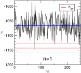
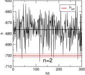
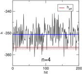
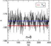
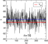
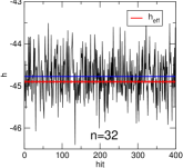
Fig. 1 shows the history of $h$ in Eq. (8). $h_{\rm eff}$ in Fig. 1 is defined by $e^{-h_{\rm eff}}=\langle e^{-h}\rangle_{\xi}$ and represented by red lines. When $n=1$, that is, we do not impose the $n^{th}$ root trick, the fluctuation of $h$ is so huge ($\sim O(10)$) that the sampling is dominated by only one hit and tends to fail. We find, however, that the magnitude of the fluctuation of $h$ behaves as $\sim 1/n$ as $n$ increases, and the sampling gets close to the situation in which $\langle h\rangle_{\xi}\sim h_{\rm eff}$ ($\langle h\rangle_{\xi}$ is represented by blue lines). Fig. 3 shows the total $H_{\rm eff}$ defined by $e^{-H_{\rm eff}}=\langle e^{-H}\rangle_{\xi}$. We find that the case $n=1$ (no root) gives a quite misleading value, and as $n$ increases, $H_{\rm eff}$ approaches an asymptotic value. Note also the jackknife errors completely underestimate the true error for small $n$. The $16^{th}$ root seems sufficient to obtain the correct value of the reweighting factor for this case.

Canceling the fluctuations

Here we discuss cancellation of the fluctuation. As a test, we consider the $4^{th}$ root of the reweighting factor, and we use two kinds of stochastic estimation:

$$w^{1/4} = \langle e^{-h_{\rm L_{1}}}\rangle_{\xi}\langle e^{-h_{\rm L_{2}}}\rangle_{\xi}\;\;\;\;\;\;{\rm or}\;\;\;\;\;\;\langle e^{-h_{\rm L_{1}L_{2}}}\rangle_{\xi},$$ (10)

where

$$\langle e^{-h_{\rm L_{2}}}\rangle_{\xi}=\det^{1/4}\left[\frac{{\cal D}_{2}(m_{f})}{{\cal D}_{2}(1)}\right],\;\langle e^{-h_{\rm L_{1}}}\rangle_{\xi}=\det^{1/4}\left[\frac{{\cal D}_{1}(1)}{{\cal D}_{1}(m_{f})}\right],\;\langle e^{-h_{\rm L_{1}L_{2}}}\rangle_{\xi}=\det^{1/4}\left[\frac{{\cal D}_{2}(m_{f})}{{\cal D}_{1}(m_{f})}\frac{{\cal D}_{1}(1)}{{\cal D}_{2}(1)}\right].$$ (11)

The history of $h_{\rm L_{1}L_{2}}$ is shown in Fig. 1 ($n=4$) and of $h_{\rm L_{1}}$ and $h_{\rm L_{2}}$ are shown in Fig. 3. While magnitude of the fluctuation of the $h_{\rm L_{1}}$ and $h_{\rm L_{2}}$ is around $200$, that of the $h_{\rm L_{1}L_{2}}$ is largely reduced to around $10$. It shows combining the determinants gives us a great advantage.

Figure 2: $n$ dependence of total $H_{\rm eff}$.

Figure 3: History of $h_{\rm L_{1}}$ and $h_{\rm L_{2}}$.

4 Fluctuation of the reweighting factor among different gauge configurations

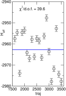
In this section we discuss the fluctuation of the reweighting factor $w$ among different gauge configurations. Even when the correct $w$ for a given configuration is obtained by the methods in previous section, too large fluctuation of $w$ among different gauge configurations could still ruin the precise estimation for the final reweighed observable. As an example, we show results of the reweighting from $L_{s}=8$ to $16$ using configurations of traj id $=1600\sim 3500$ in Conf [B] (2).

4.1 Naive fluctuations

(a) without shift

(b) with shift of $\beta$

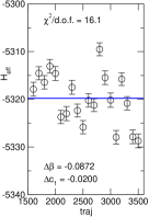(c) with shift of $\beta$, $c_{1}$

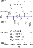(d) with shift of $\beta$, $c_{1}$, $c_{2}$ and $c_{3}$

Figure 4: $H_{\rm eff}$ in configuration to configuration.

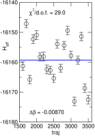
Fig. 4 (a) shows the obtained $H_{\rm eff}$ of each configurations. The blue line in the figure represents a constant fit line and its $\chi^{2}/\mbox{d.o.f.}$ is also put. While the $H_{\rm eff}$’s themselves seem to be well determined, their fluctuation among different configurations is quite large. Then we conclude that the overlap between original and desired configurations is so small that it is difficult to perform the reweighting reliably for our parameter and volume.

4.2 Shifting parameters

Now we consider to compensate the reweighting factor for the large fluctuation with shifting simulation parameters. Here we consider a gluon action with standard combination:

$$S_{\rm gluon}=-\beta\left(c_{0}[\mbox{plaquette}]+c_{1}[\mbox{rectangle}]+c_{2}[\mbox{chair}]+c_{3}[\mbox{parallelogram}]\right),$$ (12)

with $c_{0}+8c_{1}+16c_{2}+8c_{3}=1$ ($c_{1}=-0.331$ and $c_{2}=c_{3}=0$ on the original gluon configuration (Iwasaki glue)), which means that we have a parameter space $(L_{s},\beta,c_{1},c_{2},c_{3},m_{f},M_{5})$ in our simulation where $M_{5}$ denotes DW height. We, however, consider shifting parameters only in the gluon sector $\beta$, $c_{1}$, $c_{2}$ and $c_{3}$ in the reweighting here.

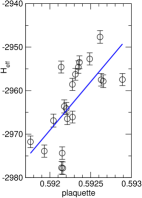(a) plaquette

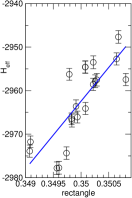(b) rectangle

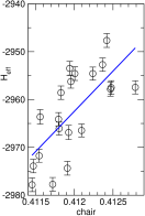(c) chair

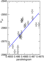(d) parallelogram

Figure 5: Correlation between $H_{\rm eff}$ and various link loops.

Fig. 5 represents the correlation of $H_{\rm eff}$ with plaquette (a), rectangle (b), chair (c) and parallelogram (d). Each quantity is likely to have a linear correlation with $H_{\rm eff}$ (the guide is shown by blue lines in each figures), which means a shift of $\beta$ could help to reduce the fluctuation. And although the trends of the figures seem to be the same, they are still slightly different, which means we could use their combination to reduce the fluctuation. Figs. 4 (b), (c) and (d) show the $H_{\rm eff}$ changed by optimised parameter shift which gives the smallest $\chi^{2}/\mbox{d.o.f.}$ in the constant fit. If we keep the value of the Iwasaki gluon parameter, and we only shift $\beta$, the reduction of $\chi^{2}/\mbox{d.o.f.}$ is small. (Fig. 4 (b)) On the other hand, we can largely reduce $\chi^{2}/\mbox{d.o.f.}$ by shifting $c_{1}$. (Fig. 4 (c)) The shift of $c_{2}$ and $c_{3}$ does not contribute to the reduction so much. (Fig. 4 (d)) While the shifting the parameters in the gluon sector can contribute to the reduction of the fluctuation, the fluctuations are so large that we are unable to perform the reweighting. This indicates that we need to shift other parameters, that is, $m_{f}$ and $M_{5}$.

4.3 Balanced reweighting

Besides shifting the parameters, an alternative idea is to balance more than one type of reweighting. While we investigate $N_{f}=2+1$ simulations, the strange quark sector has not been accounted for in this study. When the strange quark is included, we obtain an additional handle to control the fluctuations. If we consider chiral symmetry for the strange quark is less important than that for the up and down quarks, the fluctuation could be suppressed by enlarging the $L_{s}$ for the up and down quarks while reducing $L_{s}$ for the strange, assuming large cancellation of the fluctuation between the light and strange quark sector. The up and down sector and the strange sector are, as it were, well “balanced”. One of the other application of this concept might be the mass reweighting. For example, in the $N_{f}=2+1$ simulation one could reduce the fluctuations between the reweighting due to the shift of degenerate up and down sea quark mass $m_{ud}$, and that of strange sea quark mass $m_{s}$ to the first order in the mass shift $\Delta m$:

$$w(m_{ud}\rightarrow m_{ud}-\Delta m;~{}m_{s}\rightarrow m_{s}+2\alpha\Delta m)=O(\Delta m^{2}),$$ (13)

where $\alpha$ is one at $m_{ud}=m_{s}$ and is decreasing function of $(m_{s}-m_{ud})$, to be tuned by numerical calculations.

5 Summary

In this report, we discussed the possibility of the reweighting method to enlarge $L_{s}$. The reweighting factor itself can be calculated correctly by using the stochastic method, dividing the determinant into many pieces. In this study we used the $n^{th}$ root trick to control this, and we found that it works well. The problem lies on the fluctuation of the reweighting factor among different gauge configurations, which is quite large. Although we tried to make parameter shifts in the gluon sector to cure the situation, it seems not enough. We consider that additional parameter shifts, like $m_{f}$ and $M_{5}$, are needed to suppress the fluctuation. We are going to address this issue in the future.

References

- [1]
- [2] D. B. Kaplan, Phys. Lett. B 288, 342 (1992) [arXiv:hep-lat/9206013].
- [3] Y. Shamir, Nucl. Phys. B 406, 90 (1993) [arXiv:hep-lat/9303005].
- [4] D. Renfrew, T. Blum, N. Christ, R. Mawhinney and P. Vranas, arXiv:0902.2587 [hep-lat].
- [5] H. Fukaya, S. Hashimoto, K. I. Ishikawa, T. Kaneko, H. Matsufuru, T. Onogi and N. Yamada [JLQCD Collaboration], Phys. Rev. D 74, 094505 (2006) [arXiv:hep-lat/0607020].
- [6] A. Hasenfratz, R. Hoffmann and S. Schaefer, Phys. Rev. D 78, 014515 (2008) [arXiv:0805.2369 [hep-lat]].
- [7] D. J. Antonio et al. [RBC Collaboration and UKQCD Collaboration], Phys. Rev. D 77, 014509 (2008) [arXiv:0705.2340 [hep-lat]].
- [8] M. A. Clark and A. D. Kennedy, Phys. Rev. Lett. 98, 051601 (2007) [arXiv:hep-lat/0608015].
![[Uncaptioned image]](/html/1003.2182/assets/x8.png)
![[Uncaptioned image]](/html/1003.2182/assets/x9.png)