Self-consistent ac quantum transport using nonequilibrium Green functions

Abstract

We develop an approach for self-consistent ac quantum transport in the presence of time-dependent potentials at non-transport terminals. We apply the approach to calculate the high-frequency characteristics of a nanotube transistor with the ac signal applied at the gate terminal. We show that the self-consistent feedback between the ac charge and potential is essential to properly capture the transport properties of the system. In the on-state, this feedback leads to the excitation of plasmons, which appear as pronounced divergent peaks in the dynamic conductance at terahertz frequencies. In the off-state, these collective features vanish, and the conductance exhibits smooth oscillations, a signature of single-particle excitations. The proposed approach is general and will allow the study of the high-frequency characteristics of many other low-dimensional nanoscale materials such as nanowires and graphene-based systems, which are attractive for terahertz devices, including those that exploit plasmonic excitations.

I INTRODUCTION

A fundamental understanding of the physical processes controlling the complex space- and time-dependent behavior of the carrier dynamics in reduced dimensions is essential to assess the technological potential of a variety of nanomaterials for future high-speed electronic devices. Such assessment, however, requires both experimental and theoretical techniques by which high-frequency material properties, such as the dynamic (ac) conductance, can be measured or calculated.

Experimentally, much progress has been made in developing techniques to probe the rf response of nanomaterials. Among these nanomaterials, carbon nanotubes have received much attention due to their exceptional electronic transport properties at dc,DurkopNL04 ; JaveyNat03 ; AvourisMT06 ; AvourisNNT07 and the hope that these carry over to high frequencies. Measurements of the high-frequency characteristics of carbon nanotube field-effect transistors (NTFETs) AppenzellerAPL04 ; LiNL04 ; RojasNL07 ; ChasteNL08 indicate little decrease in performance up to gigahertz (GHz) frequencies. In addition, the carrier dynamics in the terahertz (THz) regime was recently probed using time-domain techniques, suggesting that the carrier dynamics is determined by single-particle rather than plasmonic properties.ZhongNNT08

Theoretically, the problem of time-dependent transport has been approached using a variety of techniques such as scattering matrix theory, BuettikerPRL93 ; BuettikerJPC93 ; PretrePBR96 ; PedersenPRB98 ; WangAPL07 Floquet methods,SambePRA73 ; BrandesPRB97 ; MartinezJPA03 ; CamaletPRL03 ; IndlekoferPRB08 ; WuJPC08 ; HoPRB09 Boltzmann transport theory,AkturkPRL07 ; AkturkJAP07 ; PaydavosiTNT09 ; PaydavosiTNT09-2 and nonequilibrium Green Functions (NEGF).JauhoPRB93 ; JauhoPRB94 ; YouPRB00 ; FranssonIJCP03 ; StefanucciPRB04 ; KurthPRB05 ; ZhouJPD05 ; ZhuPRB05 ; StefanucciJPCS06 ; HouPhysE06 ; MoldoveanuPRB07 ; MoldoveanuPRB07-2 ; SouzaPRB07 ; StefanucciPRB08 ; MaciejkoPRB06 ; MyoehaenenEPL08 ; MyoehaenenPRB09 ; StanJCP09 ; PanJPC09 ; DattaPRB92 ; AnantramPRB95 ; GuoPRL99 ; RolandPRL00 ; WangPRB03 ; WeiPRB09 ; ZhengPRB00 ; WuPRB05 ; YuJCP07 ; WangPRB09 Even though the NEGF technique has become to some extent the standard in modeling electronic quantum transport, its application to time-dependent problems has been mainly focused on simplified few-level models, DattaPRB92 ; AnantramPRB95 ; GuoPRL99 ; RolandPRL00 ; ZhengPRB00 ; WuPRB05 ; YuJCP07 ; WangPRB09 or to few-atom one-dimensional wires or molecules.ZhengPRB00 ; WuPRB05 ; YuJCP07 ; WangPRB09 While such model systems are invaluable to gain insight into the basic dynamic processes of simple quantum systems, it can be difficult to relate them to more realistic devices for three main reasons. First, the self-consistency between the charge and the potential is needed to properly determine the operation of the device in the presence of dynamic potentials. Second, it is necessary to capture the rather complex dielectric environment of real devices. Third, most approaches have focused on applying time-dependent signals at the source-drain, i.e. transport terminals, FranssonIJCP03 ; MoldoveanuPRB07 ; MoldoveanuPRB07-2 ; SouzaPRB07 rather than at the gate, a non-transport terminal. Physically, non-transport terminals do not supply the device region with charge, unlike source-drain contacts, but are coupled to the device channel only through the (self-consistent) dynamic potential, which plays a similar role as the pumping potential in the field of parametric pumping.StefanucciPRB08 ; WangPRB03

In this work, we make a first step towards solving this problem and develop a linear response theory for ac quantum transport employing nonequilibrium Green functions solved self-consistently with Poisson’s equation, when a time-dependent signal is applied at the gate terminal. We apply the approach to a NTFET and determine its high-frequency response, showing that the approach cannot only describe time-dependent, single-particle quantum transport effects, but also is able to capture the plasmonic excitations of the device.

The program of the paper is as follows: in Sec. II, we detail the formal theory for ac quantum transport and derive an effective Dyson equation describing the dynamics of the system for a time-harmonic signal at a non-transport terminal. Special attention is given to the practical calculation of the frequency-dependent charge density for which we develop a computationally efficient scheme, a prerequisite for calculating the self-consistent ac response of larger systems, as we have demonstrated previously.KienlePRL09 In Sec. III, general expressions for the ac particle current and associated conductance are derived along with a brief outline of the current partitioning scheme, GuoPRL99 and how it applies to a multi-terminal device with non-transport terminals. In Sec. IV, we apply the theory to a NTFET. There, we discuss details of the significance of the operation mode of the device, and the self-consistent feedback between charge and potential for collective excitations. Our conclusions are presented in Sec. V.

II GENERAL APPROACH

In this section we describe the development of the ac approach, which consists of three steps: 1) definition of the model Hamiltonian of the total system, 2) formulating the quantum dynamics and non-equilibrium statistics in terms of Green functions in the energy domain, and 3) self-consistent calculation of the ac charge and potential.

II.1 Model Hamiltonian

We begin by specifying the Hamiltonian operator of the system. As usual, the total system is divided into three isolated regions following the partitioning scheme of Caroli and co-workersCaroliJPC71-1 ; CaroliJPC71-2 The Hamiltonian of the entire infinite system is written as

$$H=H_{d}+H_{c}+H_{t}~{},$$ (1)

where $H_{d}$ is the Hamiltonian for the device region, $H_{c}$ refers to the two semi-infinite leads, and $H_{t}$ couples the device region to the leads. In a site representation the device Hamiltonian is given by

$$H_{d} = H_{d}^{0}+H_{d}^{DC}+H_{d}^{AC}~{},$$ (2)

where

$$H_{d}^{0} = \sum_{n}\epsilon_{n}^{0}\hat{c}_{n}^{{\dagger}}\hat{c}_{n}+\frac{1}{2}\sum_{n,m}t_{n,m}\hat{c}_{n}^{{\dagger}}\hat{c}_{m}+\mbox{h.c.}~{},$$ (3)

and

$$H_{d}^{DC} = \sum_{n}U_{n}^{DC}\hat{c}_{n}^{{\dagger}}\hat{c}_{n}~{},~{}H_{d}^{AC}=\sum_{n}U_{n}(t)\hat{c}_{n}^{{\dagger}}\hat{c}_{n}~{},$$ (4)

where $\hat{c}_{n}^{{\dagger}}$ and $\hat{c}_{n}$ refer to fermionic creation and annihilation operators at site $n$. $H_{d}^{0}$ defines the equilibrium electronic structure of the isolated system. The electron-electron interaction is approximated on the Hartree level and has two components $H_{d}^{DC}$ and $H_{d}^{AC}$, cf. Eq (4). The term $U_{n}^{DC}$ represents a spatially-varying, but time-independent electrostatic potential, such as the one present when calculating the DC properties and leads to a renormalization of the onsite energies $\epsilon_{n}^{0}$.

The new physics studied here originates from the presence of an a priori unknown time- and space-dependent potential $U_{n}(t)$ induced by externally applied time-dependent fields. As further discussed below, both $U_{n}^{DC}$ and $U_{n}(t)$ must be determined separately by solving Poisson’s equation in a self-consistent manner. In general, the approach allows to investigate the dynamic response beyond the Hartree approximation of the Coulomb interaction by including exchange and correlation functionalsWangPRB09 calculated self-consistently.

The Hamiltonian for the two contacts to the left and right ($\alpha=s,d$) of the device reads

$$H_{c}=\sum_{k,\alpha}\epsilon_{k\alpha}^{0}\hat{c}_{k\alpha}^{{\dagger}}\hat{c}_{k\alpha}~{},$$ (5)

where $\hat{c}_{k\alpha}^{{\dagger}}$ and $\hat{c}_{k\alpha}$ are fermionic creation and anihilation operators for a particle in terminal $\alpha$ in state $k$. We note that equations (3), (4), and (5) differ from those considered previously where a time-dependent source-drain bias is considered, in which case the onsite energy $\epsilon_{k\alpha}^{0}$ of the contacts become time-dependent rather than the ones of the device.

Finally, the Hamiltonian

$$H_{t}=\sum_{k\alpha,n}T_{n,k\alpha}\hat{c}_{n}^{{\dagger}}\hat{c}_{k\alpha}+T_{n,k\alpha}^{\ast}\hat{c}_{k\alpha}^{{\dagger}}\hat{c}_{n}~{},$$ (6)

couples the device sub-space with the semi-infinite source and drain reservoirs, and allows for a physical exchange of particles through the device-contact interface. Therefore, the tunneling Hamiltonian Eq. (6) describes only the coupling between the device and transport terminals, but not to non-transport terminals.

II.2 Quantum dynamics and nonequilibrium statistics

The next step is to describe the carrier dynamics within the device scattering region using Green functions. The Green functions are in general functions of both space and time, e.g. $G(\mathbf{r}t;\mathbf{r}^{\prime}t^{\prime})$. However, to simplify the equations for compactness we adopt a short-hand notation $G(t,t^{\prime})\equiv G(\mathbf{r}t;\mathbf{r}^{\prime}t^{\prime})$. In addition, whenever regular functions appear with Green functions in the same equation, we also omit the spatial dependence on the regular functions.

We start with the time-dependent Dyson equationHaug1998

$$G^{\gamma}(t,t^{\prime}) = g_{0}^{\gamma}(t,t^{\prime})$$

$$+ \int dt_{1}dt_{2}~{}g_{0}^{\gamma}(t,t_{1})\Sigma^{\gamma}(t_{1},t_{2})G^{\gamma}(t_{2},t^{\prime})~{},$$

where $g_{0}^{\gamma}(t,t^{\prime})=g_{0}^{\gamma}(t-t^{\prime})$ refers to the retarded/advanced ($\gamma=\mbox{{r},{a}}$) Green function of the isolated system. The self-energy $\Sigma^{\gamma}(t,t^{\prime})$ accounts for all interactions of the isolated system with its environment. In our case, the self-energy $\Sigma^{\gamma}(t,t^{\prime})$ can be divided into three contributions

$$\Sigma^{\gamma}(t,t^{\prime})=\sum_{\alpha=s,d}\Sigma_{\alpha}^{\gamma}(t-t^{\prime})+U^{DC}\delta(t-t^{\prime})+U(t)\delta(t-t^{\prime})~{}.$$ (8)

The first term $\Sigma_{c}\equiv\sum_{\alpha=s,d}\Sigma_{\alpha}$ is the contact self-energy and corresponds to the quantum-transport open-boundary conditions connecting the device region with the semi-infinite source and drain contacts. The second term is a scalar potential and represents the internal response of the device to externally applied time-independent fields. The third term is the prominent feature in the ac theory presented here, and describes the dynamic response of the device due to external time-dependent fields. Contrary to most studies where the ac signal is applied at the source-drain terminals,GuoPRL99 ; ZhouJPD05 ; WangPRB09 ; WeiPRB09 in our case the time-dependent signal is applied at the gate terminal. This implies that the induced potential $U(t)$ distorts only the device scattering region, while the contacts remain in steady-state.

We now switch from the time-domain into energy-representation through a double-time Fourier-transform defined asGuoPRL99

$$F(E,E^{\prime})=\int dtdt^{\prime}e^{iEt/\hbar}e^{-iE^{\prime}t^{\prime}/\hbar}F(t,t^{\prime})$$ (9)

and

$$F(t,t^{\prime})=\int\frac{dE}{2\pi}\frac{dE^{\prime}}{2\pi}e^{-iEt/\hbar}e^{iE^{\prime}t^{\prime}/\hbar}F(E,E^{\prime})~{},$$ (10)

so that the self-energy, cf. Eq. (8) is given by

$$\Sigma^{\gamma}(E,E^{\prime})=2\pi\delta(E-E^{\prime})\left[\Sigma_{c}^{\gamma}(E)+U^{DC}\right]+U(E-E^{\prime}).$$ (11)

It is worthwhile mentioning that in energy domain the contact self-energies are local in energy, reflecting that under steady-state conditions there is no mixing between states with different energy within the reservoirs. On the other hand, the original time-local potential $U$ becomes now in energy domain non-local, implying that a time-dependent potential mediates transitions between states at different energies within the device scattering region.

Fourier transforming Eq. (II.2) and using (11), one derives an effective Dyson equation for the device

$$G^{\gamma}(E,E^{\prime}) = 2\pi\delta(E-E^{\prime})G_{0}^{\gamma}(E)$$

$$+ \int\frac{d\bar{E}}{2\pi}~{}G_{0}^{\gamma}(E)U(E-\bar{E})G^{\gamma}(\bar{E},E^{\prime})~{},$$

where

$$G_{0}^{\gamma}(E) = \left[g_{0}^{\gamma}(E)^{-1}-U^{DC}-\Sigma_{c}^{\gamma}(E)\right]^{-1}~{},$$ (13)

and

$$g_{0}^{\gamma}(E) = \left[\left(E\pm i\eta\right)I-H_{d}^{0}\right]^{-1}~{},$$ (14)

with an infinitesimal $\eta>0$. What we have gained in re-formulating Dyson’s equation is to partition the full dynamic response of the system described through the two-energy Green function $G(E,E^{\prime})$ into its dc and ac components given by the first and second term in equation (II.2), respectively. Importantly, the DC component determined by the newly defined Green function $G_{0}^{\gamma}$, cf. Eq. (13), refers no longer to the response of the isolated system $g_{0}^{\gamma}$, cf. Eq. (14), but rather describes the system’s response in contact with the leads and subject to a dc electrostatic potential. Hence, $G_{0}^{\gamma}$ defines the operation point of the open system under DC steady-state. The ac component, i.e. the second term in Eq. (II.2) contains this term as well and determines the distortion of the system away from the operation point $G_{0}^{\gamma}$, and is driven by the time-dependent potential $U(t)$ leading to a coupling of states at different energies.

We still need to know how the total nonequilibrium particle distribution $G^{<}$ deviates from its (reference) distribution at dc in the presence of the ac potential $U$. This is accomplished by mapping Dyson’s equation for $G^{<}$, symbolically written as $G^{<}=\left[G_{0}+G_{0}UG\right]^{<}$, onto the real-time axis utilizing the Langreth rulesLangrethPRB72 ; Haug1998 which gives: $G^{<}=G_{0}^{<}+G_{0}^{<}UG^{a}+G_{0}^{r}UG^{<}$. This integral equation can be solved exactly making use of Eqs. (II.2) and (13). Details of the derivation are found in appendix A. After Fourier transform the particle distribution is given by

$$G^{<}(E,E^{\prime}) = 2\pi G_{0}^{<}(E)\delta(E-E^{\prime})$$

$$+ \int\frac{d\bar{E}}{2\pi}\left[G_{0}^{<}(E)U(E-\bar{E})G^{a}(\bar{E},E^{\prime})\right.$$

$$+ \left.~{}~{}~{}~{}~{}~{}~{}~{}~{}~{}G^{r}(E,\bar{E})U(\bar{E}-E^{\prime})G_{0}^{<}(E^{\prime})\right]$$

$$+ \int\frac{dE_{1}}{2\pi}\frac{dE_{2}}{2\pi}\frac{dE_{3}}{2\pi}\times$$

$$~{}~{}~{}~{}G^{r}(E,E_{1})U(E_{1}-E_{2})G_{0}^{<}(E_{2})\times$$

$$~{}~{}~{}~{}U(E_{2}-E_{3})G^{a}(E_{3},E^{\prime})~{},$$

where $G_{0}^{<}(E)=G_{0}^{r}(E)\Sigma_{c}^{<}(E)G_{0}^{a}(E)$ corresponds to the nonequilibrium spectral particle density at dc. The function $\Sigma_{c}^{<}(E)=\sum_{\alpha=s,d}if_{\alpha}(E)\Gamma_{\alpha}(E)$ where $\Gamma_{\alpha}(E)=i\left(\Sigma_{\alpha}^{r}-\Sigma_{\alpha}^{a}\right)$ is the broadening function, and $f_{\alpha}(E)=1/\left[1+e^{(E-\mu_{\alpha})/k_{B}T}\right]$ is the Fermi function at temperature $T$ with $\mu_{\alpha}$ being the chemical potential of terminal $\alpha$.

While the set of equations (II.2)-(II.2) developed so far describe entirely the quantum transport and nonequilibrium statistics, they do not allow to determine the dynamic potential $U$. This must be obtained by solving Poisson’s equation

$$\nabla\left[\epsilon(\mathbf{r})\nabla U(\mathbf{r},E-E^{\prime})\right]=-\rho(\mathbf{r},E-E^{\prime})~{},$$ (16)

with the frequency-dependent charge density

$$\rho(\omega)=ie\int\frac{dE}{2\pi}~{}G^{<}(E^{+},E)~{}.$$ (17)

The calculation of the ac charge density using Eq. (II.2) requires $G^{<}$ to be evaluated at two energies $(E^{+},E)\equiv(E+\hbar\omega,E)$, in contrast to the dc case where only one energy is needed.

Equations (16) and (17) implement the self-consistent coupling between electrostatics and transport, which represents the key component in our ac approach. Note that at the frequencies considered here the electromagnetic fields respond instantaneously, so that the full time dependence in Maxwell’s equations can be neglected. Poisson’s equation is supplemented by boundary conditions appropriate for the problem at hand, and $\epsilon(\mathbf{r})$ is a space-dependent dielectric constant that can account for more complex inhomogeneous dielectric environments quite common in devices.

The set of Eqs. (II.2)-(17) describe the nonequilibrium quantum dynamics and its coupling to Poisson’s equation for an arbitrary time-dependent potential $U$, and can thus describe situations beyond linear response, in general. However, the numerical implementation of the full non-linear theory requires the calculation of a triple energy integral in Eq. (II.2), which is prohibitive at this time given the need for self-consistency to capture the plasmonic response of real devices as discussed in Sec. IV.

II.3 Linearized equations

To proceed further, we now apply a time-harmonic signal at the gate terminal ${\tilde{v}}_{g}(t)=v_{0}\cos(\omega t)$ of small amplitude $v_{0}$ and frequency $\omega$, and seek the potential response in the form $U(\mathbf{r},t)=V(\mathbf{r},\omega)\cos(\omega t)$, which reads in energy domain

$$U(E)=\frac{1}{2}V(\mathbf{r},\omega)\left[\delta(E+\hbar\omega)+\delta(E-\hbar\omega)\right]~{}.$$ (18)

Keeping only terms to linear order in $V$, the ac transport-Poisson equations take the form

$$G^{\gamma}(E^{+},E) = 2\pi G_{0}^{\gamma}(E)\delta(\hbar\omega)+\frac{1}{2}G_{0}^{\gamma}(E^{+})V(\omega)G_{0}^{\gamma}(E),$$

$$G^{<}(E^{+},E) = 2\pi G_{0}^{<}(E)\delta(\hbar\omega)+\frac{1}{2}G_{0}^{<}(E^{+})V(\omega)G_{0}^{a}(E)$$ (20)

$$+ \frac{1}{2}G_{0}^{r}(E^{+})V(\omega)G_{0}^{<}(E)~{},$$

$$\rho(\omega) = ie\int\frac{dE}{2\pi}~{}G^{<}(E^{+},E),$$ (21)

$$-\rho(\mathbf{r},\omega) = \nabla\left[\epsilon(\mathbf{r})\nabla V(\mathbf{r},\omega)\right]~{}.$$ (22)

II.4 Numerical calculation of $\rho(\mathbf{r},\omega)$

An integral part in the self-consistent transport calculations is the determination of the charge density. In practice, one has to evaluate the integral in Eq. (21) which is often performed by direct integration along the real energy axis. In many cases, this is a sufficient approach because the spectral density of states has a finite bandwidth, thus narrowing the integration window. However, such conditions are rarely realized in more realistic device models. For instance, even in a simple tight-binding representation of a NTFET (see Sec. IV) the bandwidth of the valence and conduction band is about $10$ eV, in which case the calculation of the charge density through a real-axis integration can become prohibitive for self-consistent calculations even at dc. This becomes an even more severe bottleneck in the case of ac simulations, where now the charge has to be determined at every frequency $\omega$.

In the following, we describe a computational efficient approach, which permits the calculation of the frequency-dependent charge density $\rho(\omega)$ by exploiting contour integration in the complex energy plane.ZellerSSC82 ; BrandbygePRB02 The basic idea is similar to the dc case, i.e. to separate in Eq. (21) the zero-bias contribution to $\rho(\omega)$ from the non-zero-bias component. If we further assume that the lowest chemical potential is at the drain terminal, i.e. $\mu_{d}^{(+)}<\mu_{s}^{(+)}$ the frequency-dependent particle distribution at zero-bias (ZB) reads

$$G_{ZB}^{<}(E^{+},E) = \frac{i}{2}A_{0}^{+}V(\omega)G_{0}^{a}f_{d}^{+}+\frac{i}{2}G_{0}^{r,+}V(\omega)A_{0}f_{d}~{},$$

where a $+$ superscript indicates a function evaluated at $E+\hbar\omega$, and the absence of such a superscript indicates a function evaluated at $E$. The steady-state spectral density is given by

$$A_{0}^{(+)}=i\left[G_{0}^{r,(+)}-G_{0}^{a,(+)}\right]~{}.$$ (24)

$G_{ZB}$ contains Fermi functions evaluated a two different energies $E$ and $E^{+}$, reflecting the nonequilibrium nature of the ac charge density for finite frequencies even at zero-bias, which means that an externally applied ac signal acts as if a frequency-dependent bias were applied.

Taking advantage of this ac-signal-bias analogy and noting that $f_{d}^{+}<f_{d}$, one can split again the zero-bias particle density into its equilibrium and nonequilibrium components, i.e. $G_{ZB}^{<}=G_{ZB}^{<,eq}+G_{ZB}^{<,neq}$, which after re-arrangement take the form

$$G_{ZB}^{<,eq}=-\frac{i}{2}\left(f_{d}+f_{d}^{+}\right)~{}\mbox{Im}\left\{G_{0}^{r,+}V(\omega)G_{0}^{r}\right\}~{},$$ (25)

and

$$G_{ZB}^{<,neq} = -\frac{1}{2}\left(f_{d}-f_{d}^{+}\right)\left[\mbox{Re}\left\{G_{0}^{r,+}V(\omega)G_{0}^{r}\right\}\right.$$

$$~{}~{}~{}~{}~{}~{}~{}~{}~{}~{}~{}~{}~{}~{}~{}~{}~{}~{}~{}~{}~{}~{}~{}\left.-G_{0}^{r,+}V(\omega)G_{0}^{a}\right]~{}.$$

The equilibrium part $G_{ZB}^{<,eq}$ is analytic in the upper complex plane, since it consists of the product of two retarded Green functions $G_{0}^{r}$ and $G_{0}^{r,+}$ each of which has poles only in the lower complex plane.Haug1998 Therefore, the equilibrium zero-bias ac particle density, which involves all states below the frequency-dependent chemical potential $\mu_{d}^{+}$, can be efficiently calculated through integration over a complex energy contour.ZellerSSC82 ; BrandbygePRB02 Conversely, the nonequilibrium component at zero-bias $G_{ZB}^{<,neq}$ is non-analytic, because both the retarded and the advanced Green functions are needed with their corresponding poles located in the lower and upper complex plane, respectively. However, this does not pose a serious problem in practice as the integration range is limited to a finite energy window given by $\hbar\omega$, i.e. the difference between the chemical potentials $\mu_{d}-\mu_{d}^{+}$.Note3

III ac RESPONSE FUNCTIONS: CURRENT AND CONDUCTANCE

The set of equations (LABEL:EqAC:GR)-(22) developed in the previous section allow the determination of the frequency-dependent Green functions, which can now be used to obtain ac response functions. One basic response function to characterize transport is the dynamic conductance $g_{\alpha\beta}$, which relates the total ac current $I_{\alpha}$ with the voltage applied at terminal $\beta$. Under time-dependent conditions this conductance is not entirely determined by the particle current, but has in general contributions from the displacement current as well. In the following subsections, we derive an expression for the particle conductance, and summarize how displacement currents can be included in the total conductance.

III.1 Particle current $I_{\alpha}^{p}(\omega)$

The first contribution to the total current consists of the flow of charged particles through the terminal $\alpha$, and is hence determined by the dynamic change of the particle density at this terminal

$$I_{\alpha}^{p}(t)=-e\frac{d}{dt}\langle\hat{N}_{\alpha}(t)\rangle=-e\frac{d}{dt}\sum_{k}\langle\hat{c}_{k\alpha}^{{\dagger}}(t)\hat{c}_{k\alpha}(t)\rangle~{}.$$ (27)

Making use of the fermionic anti-commutator relations,Haug1998 and the Heisenberg equation of motion for operators $\dot{\mathcal{O}}=\frac{i}{\hbar}\left[H,\mathcal{O}\right]$ with $H$ the total system Hamiltonian, cf. Eq. (1), one derives the well-known matrix equation for the equal-time particle currentJauhoPRB94 ; AnantramPRB95 ; WeiPRB09

$$I_{\alpha}^{p}(t) = \frac{e}{\hbar}Tr\int dt^{\prime}\left[G^{r}(t,t^{\prime})\Sigma_{\alpha}^{<}(t^{\prime},t)-\Sigma_{\alpha}^{<}(t,t^{\prime})G^{a}(t^{\prime},t)\right.$$ (28)

$$+ \left.G^{<}(t,t^{\prime})\Sigma_{\alpha}^{a}(t^{\prime},t)-\Sigma_{\alpha}^{r}(t,t^{\prime})G^{<}(t^{\prime},t)\right]~{}.$$

Its corresponding energy representation readsJauhoPRB94 ; AnantramPRB95 ; GuoPRL99

$$I_{\alpha}^{p}(\omega) = \frac{e}{\hbar}Tr\int\frac{dE}{2\pi}\frac{dE^{\prime}}{2\pi}\left[G^{<}(E^{+},E^{\prime})\Sigma_{\alpha}^{a}(E^{\prime},E)\right.$$ (29)

$$- \left.\Sigma_{\alpha}^{r}(E^{+},E^{\prime})G^{<}(E^{\prime},E)+G^{r}(E^{+},E^{\prime})\Sigma_{\alpha}^{<}(E^{\prime},E)\right.$$

$$- \left.\Sigma_{\alpha}^{<}(E^{+},E^{\prime})G^{a}(E^{\prime},E)\right]~{}.$$

Equation (29) simplifies further if we exploit the steady-state property of the contact self-energies from Eq. (11) in which case one obtains the frequency-dependent particle current

$$I_{\alpha}^{p}(\omega) = \frac{e}{h}Tr\int dE\left[G^{<}(E^{+},E)\Sigma_{\alpha}^{a}(E)\right.$$ (30)

$$- \left.\Sigma_{\alpha}^{r}(E^{+})G^{<}(E^{+},E)+G^{r}(E^{+},E)\Sigma_{\alpha}^{<}(E)\right.$$

$$- \left.\Sigma_{\alpha}^{<}(E^{+})G^{a}(E^{+},E)\right]~{}.$$

We note that the expression for $I_{\alpha}^{p}(\omega)$ differs from those derived in Refs.AnantramPRB95 ; GuoPRL99 ; WeiPRB09 , since those applied a time-dependent voltage at the source-drain, instead of the gate excitation considered here.

One can now derive the dynamic particle conductance by expanding $\Sigma_{\alpha}^{<}$ and $G^{<}$ appearing in Eq. (30) to linear order in the terminal voltage $v_{\beta}$, and utilizing Eq. (LABEL:EqAC:GR) and (20) to substitute for $G^{\gamma}(E^{+},E)$ and $G^{<}(E^{+},E)$. These linearized expressions are summarized in Appendix B. Inserting all relevant terms in Eq. (30) and keeping components linear in $V(\omega)$, we derive for the frequency-dependent particle current

$$I_{\alpha}^{p}(\omega) = \frac{1}{2}\frac{e^{2}}{h}\sum_{\beta}Tr\int dE\left[\left\{G_{0}^{r,+}V(\omega)G_{0}^{r}\widetilde{\Sigma}_{\beta}^{<}-\widetilde{\Sigma}_{\beta}^{<,+}G_{0}^{a,+}V(\omega)G_{0}^{a}\right\}\delta_{\alpha\beta}\right.$$

$$+ \left.\widetilde{G}_{0,\beta}^{<,+}V(\omega)G_{0}^{a}\Sigma_{\alpha}^{a}+G_{0}^{r,+}V(\omega)\widetilde{G}_{0,\beta}^{<}\Sigma_{\alpha}^{a}-\Sigma_{\alpha}^{r,+}\widetilde{G}_{0,\beta}^{<,+}V(\omega)G_{0}^{a}-\Sigma_{\alpha}^{r,+}G_{0}^{r,+}V(\omega)\widetilde{G}_{0,\beta}^{<}\right]~{}v_{\beta}~{}~{}.$$

By definition, the (tensor) prefactor that relates the terminal current $I_{\alpha}$ with the applied bias $v_{\beta}$ is the ac linear response particle conductance, and can be read directly from Eq. (III.1):

$$g_{\alpha\beta}^{p}(\omega) = \frac{1}{2}\frac{e^{2}}{h}Tr\int dE\left[\left\{G_{0}^{r,+}V(\omega)G_{0}^{r}\widetilde{\Sigma}_{\beta}^{<}-\widetilde{\Sigma}_{\beta}^{<,+}G_{0}^{a,+}V(\omega)G_{0}^{a}\right\}\delta_{\alpha\beta}\right.$$

$$+ \left.\widetilde{G}_{0,\beta}^{<,+}V(\omega)G_{0}^{a}\Sigma_{\alpha}^{a}+G_{0}^{r,+}V(\omega)\widetilde{G}_{0,\beta}^{<}\Sigma_{\alpha}^{a}-\Sigma_{\alpha}^{r,+}\widetilde{G}_{0,\beta}^{<,+}V(\omega)G_{0}^{a}-\Sigma_{\alpha}^{r,+}G_{0}^{r,+}V(\omega)\widetilde{G}_{0,\beta}^{<}\right]~{}.$$

III.2 Displacement current $I^{d}(\omega)$

Under time-dependent conditions the particle conductance does not in general obey sum-rules, i.e. $\sum_{\alpha}g_{\alpha\beta}=0$ and $\sum_{\beta}g_{\alpha\beta}=0$, reflecting current continuity and gauge-invariance, because the displacement current present under ac conditions is often discarded. The current partitioning scheme of Wang et al.GuoPRL99 allows to re-establish these sum-rules by taking displacement currents into account.

The basic idea of this scheme can be summarized as follows: starting from the charge continuity equation, $\partial_{t}\rho+\nabla\cdot\mathbf{j}^{p}=0$, and integrating over the volume one obtains Kirchoff’s current law, i.e. $I^{d}(t)+\sum_{\alpha}I_{\alpha}^{p}=0$. $I_{\alpha}^{p}$ refers to the particle current through terminal $\alpha$, and can be associated with a particle conductance through $I_{\alpha}^{p}=\sum_{\beta}g_{\alpha\beta}^{p}v_{\beta}$ with $v_{\beta}$ the voltage at terminal $\beta$. The displacement current $I^{d}(t)=\partial_{t}Q(t)$ accounts for the dynamic change of the total charge, and is non-zero under time-dependent conditions.

To obtain an expression for the total conductance defined by $I_{\alpha}=\sum_{\beta}g_{\alpha\beta}v_{\beta}$ one needs to know how the current $I_{\alpha}$ is split between the particle and the displacement current at each terminal. While the particle component $I_{\alpha}^{p}$ is directly accessible through transport, this is not immediately possible for $I^{d}$, since only the total rather than the terminal displacement current is known. This problem can be resolved by making two Ansätze for the terminal and total displacement current,GuoPRL99 i.e. $I_{\alpha}:=I_{\alpha}^{p}+A_{\alpha}I^{d}$ and $I^{d}:=\sum_{\beta}g_{\beta}^{d}v_{\beta}$, where $g_{\beta}^{d}$ defines the displacement conductance, and permits to specify a total conductance: $g_{\alpha\beta}=g_{\alpha\beta}^{p}+A_{\alpha}g_{\beta}^{d}$. The partitioning factor $A_{\alpha}$ can be determined by employing the sum-rules $\sum_{\alpha}g_{\alpha\beta}=0$ and $\sum_{\beta}g_{\alpha\beta}=0$, so that the total conductance is given byGuoPRL99

$$g_{\alpha\beta}=g_{\alpha\beta}^{p}-\frac{\sum_{\gamma}g_{\alpha\gamma}^{p}}{\sum_{\gamma}g_{\gamma}^{d}}g_{\beta}^{d}~{},$$ (33)

and constitutes a $(N\times N)$-matrix for a system with $N$-terminals, in general.

IV APPLICATION: NANOTUBE FET

In this section, we apply the approach developed in the previous sections to a ballistic nanotube transistor shown in Fig. 1 with a channel length of $L=20$ nm. In general, the high-frequency properties of this three-terminal device can be determined by any component of the $(3\times 3)$-conductance matrix, cf. Eq. (33); here we chose the source-drain conductance $g_{sd}(\omega)$ calculated at zero-bias and $T=300$ K.

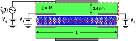
Figure 1: (Color online). Cross section of the NTFET device in cylindrical geometry and embedded in a dielectric medium. The dashed rectangle specifies the computational domain.

Since the ac signal is applied only at the gate terminal, which couples capacitively to the nanotube channel, one can assume that the dominant contribution to the displacement current is carried by the gate, i.e. $I^{d}\approx I_{g}$. In this case, the partitioning factors for the three terminals simplify, i.e. $(A_{s},A_{d},A_{g})\approx(0,0,1)$, so that the source-drain ac conductance is given by $g_{sd}(\omega)\approx g_{sd}^{p}(\omega)$. Here, we focus on one particular channel length to discuss aspects of the methodology that are essential for the proper description of the ac behavior. The properties of such devices with different dimensions were presented by us in detail in Ref. KienlePRL09 .

IV.1 Transistor response in the dc operation point

We begin our analyis by specifying the setup of the device shown in Figure 1 following the modeling approach of Ref.LeonardNT06 . The channel, which consist of a semi-conducting tube with chirality $(m,n)=(17,0)$ and radius $0.66$ nm, is placed in the center of a cylindrical hole with radius $0.96$ nm and surrounded by a dielectric with a permittivity of $16$ ($\mbox{HfO}_{2}$).

The equilibrium electronic structure of the nanotube is described within a $p_{z}$ tight-binding model with diagonal matrix elements $\epsilon_{i,i}^{0}=0$, and off-diagonal elements $t_{2i,2i-1}=t_{2i-1,2i}=2\gamma\cos\left(\frac{\pi J}{m}\right)$, $t_{2i,2i+1}=t_{2i+1,2i}=\gamma$, where $m$ refers to the number of carbon atoms per ring. The periodic boundary conditions along the tube circumference leads to a quantization of the wavefunction, so that the NT electronic structure can be classified by an angular momentum $J=1,\ldots,m$ labeling the subbands. We chose $\gamma=2.5$ eV for the $\pi$ carbon-carbon bond energy, so that the bandgap between the highest valence and lowest conduction band ($J=6$) is $E_{g}=0.55$ eV.LeonardNT06

The contacts are semi-infinite extensions of the NT channel, and described through self-energies $\Sigma^{r}_{\alpha}=\gamma^{2}g_{\alpha}^{r}$ for each contact ($\alpha=s,d$) where $\gamma$ couples the first/last ring of the NT channel to the surface of the contacts to the left and right.LeonardNT06 The surface Green function $g_{\alpha}^{r}$ is calculated numerically at each energy using a matrix iterative scheme.SanchoJPF85 The matrix elements of the retarded Green function $G_{0}^{r}$ for the NT channel are obtained employing a recursive algorithm.SvizhenkoJAP02 The function of the two embedding metallic regions is to electrostatically dope the ends of the NT channel. In all simulations, the equilibrium Fermi level of the semi-infinite NT source/drain contacts $E_{F}$ is set at $-1.0$ eV below the NT midgap energy before self-consistency, which gives after self-consistency p-type Ohmic contacts.

Due to the cylindrical symmetry, the 3D Poisson’s equation Eq. (22) reduces to a two-dimensional (2D) problem. In this case, Poisson’s equation is discretized along the axial and radial axis within the 2D simulation domain as marked by the rectangular box using finite-differences,LeonardNT06 and the resulting linear matrix system is solved by successive overrelaxation.Press1992 Along the domain boundary we impose homogeneous von Neumann boundary conditions for the electrostatic potential ($\nabla V=0$), and use Dirichlet boundary conditions ($V=const.$) at the perfect-metal source, drain, and gate terminals. Poisson’s equation requires a 3D charge density in real-space as input. However, an orthogonal tight-binding representation of the NEGF transport equations calculates the total charge per NT ring. A 3D charge density can be obtained by smearing of the total charge per ring along the axial and radial direction of the 2D domain using Gaussian smearing functions.LeonardNT06

The first step in determining the AC response of the transistor is to choose an operation point either in the off or on state, which is controlled by an appropriate DC gate bias $V_{g}$.

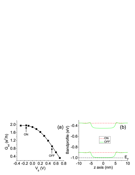
Figure 2: (Color online). (a) dc output characteristics for $L=20$ nm NTFET. The arrows mark the operation point in the on and off state, while panel (b) shows the respective self-consistent bandprofiles. The dashed-dotted line is the Fermi level with $E_{F}=-1$ eV.

Figure 2 (a) shows the output characteristics for our NTFET specified by the dc source-drain conductance $G_{sd}$ in the absence of a gate perturbation ($v_{0}=0$) with arrows marking the selected on and off states. At zero frequency, the conductance $g_{sd}(\omega=0)$ examined in the forthcoming sections is related to $G_{sd}$ by its slope taken at the operation point, i.e. $g_{sd}(\omega=0)\approx\frac{\partial G_{sd}}{\partial V_{g}}v_{0}$. Figure 2 (b) displays the respective dc bandprofiles with the band being flat in the on state leading to a maximum conductance of $2e^{2}/h$ (per spin) whereas in the off state the hole current is reduced due to the gate-controlled barrier in the channel.

IV.2 Transistor response in the off-state

We now superpose an ac signal of small amplitude $v_{0}=10$ meV and frequency $\omega$ to the dc gate bias $V_{g}$. Figure 3 (a) shows the dynamic conductance in the off state, with real and imaginary parts having oscillatory character as a function of frequency $\omega$. One can understand this behavior from the space- and energy-dependent 2D density-of-states (DOS) shown in Fig 3 (b).

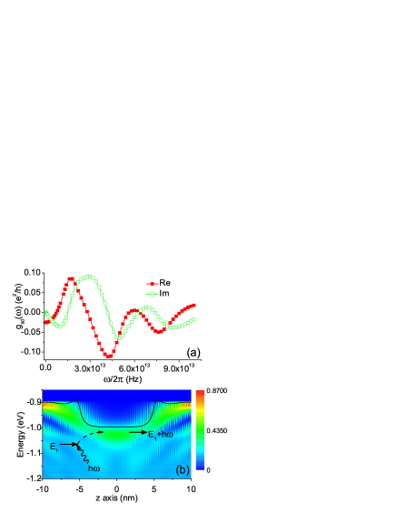
Figure 3: (Color online). ac response for a $L=20$ nm NTFET in the off state: (a) real/imaginary part of the frequency-dependent conductance, and (b) color plot of the NTFET 2D density-of-states illustrating the resonant photoexcitation of carriers between spatially and energetically oscillating states. The solid black line marks the valence band edge, and the Fermi level is $E_{F}=-1$ eV.

For a given position $z$ along the tube the DOS oscillates in energy due to the quantum interference of states by the barriers. Photoexcitations of carriers between states associated with maxima in the DOS lead to maxima in $g_{sd}(\omega)$, while its minima are caused by transitions between maxima and minima.KienlePRL09 An oscillatory behavior of the conductance is hence a signature of single-particle excitations, and is preserved when the self-consistent feedback is disabled as will be shown further below. We note that at low frequencies the real part of the conductance is negative. This is because in the limit $\omega\rightarrow 0$ the ac signal perturbation $\tilde{v}_{g}(t)=v_{0}\cos(\omega t)$ becomes effectively a positive DC bias $\tilde{v}_{g}(t)=v_{0}>0$ superposed to $V_{g}$. According to the dc transfer characteristics of Fig. 2 (a) $\partial G_{sd}/\partial V_{g}<0$, so that an increase of $V_{g}$ by $v_{0}$ leads to a reduction in the conductance.

IV.3 Transistor response in the on-state

The dynamic response is quite different in the on state as shown in Figure 4 (a). For small frequencies the dynamic conductance is slightly negative for the same reason as in the off state, and exhibits a pronounced divergence at a discrete frequency of about $\approx 36$ THz. Away from this resonance the conductance is oscillatory similar to the off state, as shown more clearly in the inset of Fig. 4 (a).

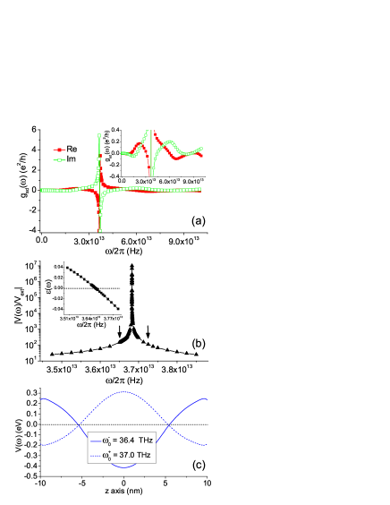
Figure 4: (Color online). ac response for a NTFET with $L=20$ nm in the on state. Panel (a) shows the real/imaginary part of $g_{sd}(\omega)$ with an enlarged view of the data shown in the inset. Panel (b): Amplitude of the normalized potential $|V(\omega)/V_{ext}|$ with the dielectric function $\epsilon(\omega)$ shown in the inset. The arrows mark the near-resonance frequencies $\omega_{0}^{\pm}$. Panel (c) shows the large amplitude potential profile $V(\omega)$ for $\omega_{0}^{\pm}$.

In order to identify the nature of this resonance, we determine the response of the electrostatic potential $V(\omega)$ for fine-sampled frequencies near the divergent behavior. In Figure 4 (b) we show the ratio of $V(\omega)/V_{ext}$ with $V_{ext}$ the external perturbing potential. Interestingly, upon approaching the resonance the amplitude of the potential diverges, cf. Fig. 4 (b). Alternatively, one can evaluate the frequency-dependent dielectric screening $\epsilon(\omega)=V_{ext}/V(\omega)$ shown in the inset of Fig. 4 (b), which has a clear zero crossing at $\omega_{0}$, while the potential undergoes a change in sign as displayed in Fig. 4 (c). These observations verify that the divergent behavior of the dynamic conductance observed in the on state is attributed to the excitation of plasmons which co-exist with the single-particle excitations.

IV.4 Importance of self-consistency

In the previous section, we were able to identify the basic features in the dynamic conductance such as the oscillatory and divergent characteristics with the single-particle and collective behavior of the channel electrons, and concluded that plasmons can only be excited if the device is operated in the on state.

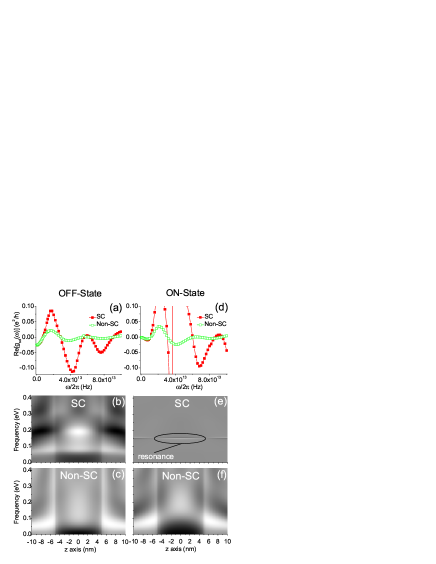
Figure 5: (Color online). Comparison of the self-consistent (SC) vs. Non-self-consistent (Non-SC) response for a $L=20$ nm NTFET. Panels (a)-(c) is the response in the off-state, with panel (a) the conductance and panels (b) and (c) the charge density. Panels (d)-(e) show the behavior in the on-state.

Are there other, more fundamental prerequisites irrespective of the operation point, which determine whether the system can be driven into a collective state at all? The answer is yes, and is related to the self-consistency between charge and potential. In Figure 5 we compare the conductance $g_{sd}(\omega)$ and the frequency-dependent charge density $\rho(z,\omega)$ calculated using the full self-consistent (SC) and a non-self-consistent approach where in the latter case the dynamic conductance is calculated in one step from the dc band profile.

In the off state, the most apparent difference between the SC vs non-SC case is that, while the SC amplitude of the conductance is larger, the smooth oscillatory behavior is preserved as shown in Fig. 5 (a). Hence, the single-particle excitation spectrum is - at least qualitatively - not affected by the charge-potential feedback. This is also apparent in the ac charge density $\rho(z,\omega)$, cf. Figs. 5 (b) and (c), which exhibits space- and frequency-dependent oscillations in both the SC- and non-SC case.

In the on state, eliminating the feedback loop has a quite different impact on the response as demonstrated in Fig. 5 (d). The plasmonic component visible through a divergent conductance $g_{sd}(\omega)$ with SC vanishes for the non-SC calculation. This drastic change in the response from the (divergent) plasmon-dominated to single-particle characteristics is again clearly reflected in the ac charge density $\rho(z,\omega)$ calculated with (SC) and without (Non-SC) feedback shown in Figs. 5 (e) and (f). In the SC case, the charge density has a large amplitude at resonance with a peak in the middle of the channel, a feature that is absent in the non-SC calculation.

V CONCLUSIONS

We develop an approach for ac quantum transport within the nonequilibrium Green function formalism, which allows to determine the frequency-dependent charge and potential under excitation at a non-transport terminal within a fully self-consistent framework.

The capability of our approach to determine the high-frequency properties of systems in complex environments is demonstrated using a nanotube transistor with an ac signal applied at its gate terminal. In the off state, the dynamic conductance shows oscillations that originate from single-particle excitations between quantized energy levels. When the device is operated in the on state, the dynamic conductance exhibits discrete divergent peaks at terahertz frequencies. These peaks are associated with plasmonic excitations of the charge density at the resonant frequencies of the transistor acting as a quantum cavity. It is shown that the self-consistent coupling between charge and potential is an essential component in the ac transport theory to capture plasmon excitations of the system. A non-self-consistent approach misses this important physics, and can only provide information about the single-particle excitation spectrum.

The proposed approach is not limited to study the ac response of nanotube devices, but can be applied to explore nonequilibrium, time-dependent electronic and optical processes in other low-dimensional materials such as nanowires, graphene, or molecules, including the exploration of their collective excitation modes for novel plasmon-based nanoscale devices.

VI ACKNOWLEDGMENT

It is a pleasure to acknowledge discussions with Mark Lee, Clark Highstrete, and Eric Shaner. This work was supported by the Laboratory Directed Research and Development program at Sandia National Laboratories. Sandia is a multiprogram laboratory operated by Sandia Corporation, a Lockheed Martin Co., for the United States Department of Energy under Contract No. DEAC01-94-AL85000. M.V. was supported at the University of Alberta by the Natural Sciences and Engineering Research Council (NSERC) of Canada.

Appendix A DERIVATION OF THE NONEQUILIBRIUM PARTICLE DENSITY $G^{<}$

In the following we detail the derivation for the particle density $G^{<}(E,E^{\prime})$, cf. Eq. (II.2). We start from the expression for the (time-domain) Dyson equation for $G^{<}$ mapped onto the real axis utilizing Langreth rules,Haug1998 ; LangrethPRB72 and symbolically written as

$$G^{<}=\left(G_{0}+G_{0}UG\right)^{<}=G_{0}^{<}+G_{0}^{<}UG^{a}+G_{0}^{r}UG^{<}$$ (34)

where we have used that $U^{<}=U(\tau)\delta^{<}(\tau-\tau^{\prime})=0$ for a time-local potential.Haug1998 This equation can be re-arranged by collecting the $G_{0}^{<}$ terms first

$$G^{<}=G_{0}^{<}\left(1+UG^{a}\right)+G_{0}^{r}UG^{<}~{}.$$ (35)

Equation (35) can be solved through iteration by inserting the expression for $G^{<}$ on the l.h.s. into the second term on the r.h.s., and collecting now the $G_{0}^{<}\left(1+UG^{a}\right)$ elements. After the first iteration one obtains

$$G^{<}=\left(1+G_{0}^{r}U\right)G_{0}^{<}\left(1+UG^{a}\right)+G_{0}^{r}UG_{0}^{r}UG^{<}~{}.$$ (36)

The retarded Green function $G_{0}^{r}$ in the prefactor $(1+G_{0}^{r}U)$ is the first term in Dyson’s series, $G^{r}=G_{0}^{r}+G_{0}^{r}UG^{r}$, which becomes more transparent when iterating one more time

$$G^{<} = \left(1+G_{0}^{r}U+G_{0}^{r}UG_{0}^{r}U\right)G_{0}^{<}\left(1+UG^{a}\right)$$

$$+ G_{0}^{r}UG_{0}^{r}UG_{0}^{r}UG^{<}$$

$$= \left[1+\left(G_{0}^{r}+G_{0}^{r}UG_{0}^{r}\right)U\right]G_{0}^{<}\left(1+UG^{a}\right)$$ (38)

$$+ G_{0}^{r}UG_{0}^{r}UG_{0}^{r}UG^{<}~{}.$$ (39)

Iterating to infinite order, this Dyson series converges towards $G^{r}$, so that the final expression for the non-equilibrium particle density reads

$$G^{<}=\left(1+G^{r}U\right)G_{0}^{<}\left(1+UG^{a}\right)~{}.$$ (40)

Equation (II.2) in section II.B corresponds to Eq. (40) after Fourier transform.

Appendix B Small Bias Expressions for $G^{<}$ and $\Sigma_{c}^{<}$

The conductance associated with the particle and displacement current are response functions which relate the terminal current $I_{\alpha}$ with the terminal voltage $v_{\beta}$ in a linear manner. In order to derive a formula for the conductance $g_{\alpha\beta}^{p}$ given in section III, one needs linearized expressions for $\Sigma^{<}$ and $G^{<}$. These can be easily obtained from the Taylor expansion of the Fermi function $f_{\beta}\equiv f_{\beta}(E)=1/\left[1+e^{(E-\mu_{\beta,0}+ev_{\beta})/k_{B}T}\right]$ to first order in the terminal voltages $v_{\beta}$, i.e.

$$f_{\beta}\approx f_{\beta,0}+e\tilde{f}_{\beta}~{}v_{\beta}~{},~{}\tilde{f}_{\beta}=-\frac{1}{k_{B}T}~{}f_{\beta,0}\left(1-f_{\beta,0}\right)~{},$$ (41)

where $\mu_{\beta,0}$ is the chemical potential of terminal $\beta$ at zero bias, and $f_{\beta,0}=1/\left[1+e^{(E-\mu_{\beta,0})/k_{B}T}\right]$ the corresponding Fermi function. Inserting Eq. (41) into $\Sigma^{<}$ and $G^{<}$ one obtains the following set of linearized expressions

$$\Sigma_{\beta}^{<} = if_{\beta}\Gamma_{\beta}=\Sigma_{\beta,0}^{<}+\widetilde{\Sigma}_{\beta}^{<}~{}v_{\beta}$$ (42)

$$\Sigma_{\beta,0}^{<} = i\Gamma_{\beta}f_{\beta,0}~{}~{},~{}~{}\widetilde{\Sigma}_{\beta}^{<}=i\Gamma_{\beta}\tilde{f}_{\beta}$$ (43)

and

$$G_{0}^{<} = \sum_{\beta=s,d}G_{0}^{r}if_{\beta}\Gamma_{\beta}G_{0}^{a}=\bar{G}_{0}^{<}+\sum_{\beta=s,d}\widetilde{G}_{0,\beta}^{<}~{}v_{\beta}$$ (44)

$$\bar{G}_{0}^{<} = \sum_{\beta=s,d}G_{0}^{r}\Sigma_{\beta,0}^{<}G_{0}^{a}~{}~{},~{}~{}\widetilde{G}_{0,\beta}^{<}=G_{0}^{r}\widetilde{\Sigma}_{\beta}^{<}G_{0}^{a}~{},$$ (45)

with $\Gamma_{\beta}=i\left(\Sigma_{\beta}^{r}-\Sigma_{\beta}^{a}\right)$ the broadening function.

References

- (1) T. Dürkop, S. A. Getty, E. Cobas, and M. S. Fuhrer, Nano Lett. 4, 35 (2004).
- (2) A. Javey, J. Guo, Q. Wang, M. Lundstrom, and H. Dai, Nature (London) 424 654 (2003).
- (3) P. Avouris and J. Chen, Mater. Today 9, 46 (2006).
- (4) P. Avouris, Z. Chen, and V. Perebeinos, Nat. Nanotechnol. 2, 605 (2007).
- (5) J. Appenzeller and D. J. Frank, Appl. Phys. Lett. 84, 1771 (2004).
- (6) S. Li, Z. Yu, S.-F. Yen, W. C. Tang, and P. J. Burke, Nano Lett. 4, 753 (2004).
- (7) L. Gomez-Rojas, S. Bhattacharyya, E. Mendoza, D. C. Cox, J.M. Rosolen, and S.R.P. Silva, Nano Lett. 7, 2672 (2007).
- (8) J. Chaste, L. Lechner, P. Morfin, G. Feve, T. Kontos, J.-M. Berroir, D. C. Glattli, H. Happy, P. Hakonen, and B. Placais, Nano Lett. 8, 525 (2008).
- (9) Z. Zhong, N. M. Gabor, J. E. Sharping, A. L. Gaeta, and P. L. McEuen, Nature Nanotechnol. 3, 201 (2008).
- (10) M. Büttiker, A. Prêtre, and H. Thomas, Phys. Rev. Lett. 70, 4114 (1993).
- (11) M. Büttiker, J. Phys.: Condens. Mat. 5, 9361 (1993).
- (12) A. Prêtre, H. Thomas, and M. Büttiker, Phys. Rev. B 54, 8130 (1996).
- (13) M. H. Pedersen, S. A. van Langen, and M. Büttiker, Phys. Rev. B 57, 1838 (1998).
- (14) L. G. Wang and K. S. Chan, Appl. Phys. Lett. 91, 063128 (2007).
- (15) H. Sambe, Phys. Rev. A 7, 2203 (1973).
- (16) T. Brandes, Phys. Rev. B 56, 1213 (1997).
- (17) D. F. Martinez, J. Phys. A 36, 9827 (2003).
- (18) S. Camalet, J. Lehmann, S. Kohler, and P. Hänggi, Phys. Rev. Lett. 90, 210602 (2003).
- (19) K. M. Indlekofer, R. Nemeth, and J. Knoch, Phys. Rev. B 77, 125436 (2008).
- (20) B. H. Wu and J. C. Cao, J. Phys.: Condens. Mat. 20, 085224 (2008).
- (21) T.-S. Ho, S.-H. Hung, H.-T. Chen, and S.-I. Chu, Phys. Rev. B 79, 235323 (2009).
- (22) A. Akturk, N. Goldsman, G. Pennington, and A. Wickenden, Phys. Rev. Lett. 98, 166803 (2007).
- (23) A. Akturk, N. Goldsman, and G. Pennington, J. Appl. Phys. 102, 073720 (2007).
- (24) N. Paydavosi, K. D. Holland, M. M. Zargham, and M. Vaidyanathan, IEEE Trans. Nanotechnol. 8, 234 (2009).
- (25) N. Paydavosi, M. M. Zargham, K. D. Holland, C. M. Dublanko, and M. Vaidyanathan, IEEE Trans. Nanotechnol., in press, doi: 10.1109/TNANO.2009.2032918.
- (26) N. S. Wingreen, A.-P. Jauho, and Y. Meir, Phys. Rev. B 48, 8487 (1993).
- (27) A.-P. Jauho, N.S. Wingreen, and Y. Meir, Phys. Rev. B 50, 5528 (1994).
- (28) J. Q. You, C.-H. Lam, and H. Z. Zheng, Phys. Rev. B 62, 1978 (2000).
- (29) J. Fransson, Int. J. Quant. Chem. 92, 471 (2003).
- (30) G. Stefanucci and C.-O Almbladh, Phys. Rev. B 69, 195318 (2004).
- (31) S. Kurth, G. Stefanucci, C.-O. Almbladh, A. Rubio, E. K. U. Gross, Phys. Rev. B 72, 035308 (2005).
- (32) S. Zhou, J. Jiang, and Q. Cai, J. Phys. D 38, 255 (2005).
- (33) Y. Zhu, J. Maciejko, T. Ji, H. Guo, and J. Wang, Phys. Rev. B 71, 075317 (2005).
- (34) G. Stefanucci and C.-O Almbladh, J. Phys.: Conf. Ser. 35, 17 (2006).
- (35) D. Hou, Y. He, X. Liu, J. Kang, J. Chen, and R. Han, Physica E 31, 191 (2006).
- (36) V. Moldoveanu, V. Gudmundsson, and A. Manolescu, Phys. Rev. B 76, 085330 (2007).
- (37) V. Moldoveanu, V. Gudmundsson, and A. Manolescu, Phys. Rev. B 76, 165308 (2007).
- (38) F. M. Souza, S. A. Leao, R. M. Gester, and A.-P. Jauho, Phys. Rev. B 76, 125318 (2007).
- (39) G. Stefanucci, S. Kurth, A. Rubio, and E. K. U. Gross, Phys. Rev. B 77, 075339 (2008).
- (40) J. Maciejko, J. Wang, and H. Guo, Phys. Rev. B 74, 085324 (2006).
- (41) P. Myöhänen, A. Stan, G. Stefanucci, and R. van Leeuwen, EPL 84, 67001 (2008).
- (42) P. Myöhänen, A. Stan, G. Stefanucci, and R. van Leeuwen, Phys. Rev. B 80, 115107 (2009).
- (43) A. Stan, N. E. Dahlen, and R. van Leeuwen, J. Chem. Phys. 130, 224101 (2009).
- (44) H. Pan and Y. Zhao, J. Phys.: Condens. Mat. 21, 265501 (2009).
- (45) S. Datta and M. P. Anantram, Phys. Rev. B 45, 13761 (1992).
- (46) M. P. Anantram and S. Datta, Phys. Rev. B 51, 7632 (1995).
- (47) B. Wang, J. Wang, and H. Guo, Phys. Rev. Lett. 82, 398 (1999).
- (48) C. Roland, M. B. Nardelli, J. Wang, and H. Guo, Phys. Rev. Lett. 84, 2921 (2000).
- (49) B. Wang, J. Wang, and H. Guo, Phys. Rev. B 68, 155326 (2003).
- (50) Y. Wei and J. Wang, Phys. Rev. B 79, 195315 (2009).
- (51) W. Zheng, Y. Wei, J. Wang, and H. Guo, Phys. Rev. B 61, 13121 (2000).
- (52) J. Wu, B. Wang, J. Wang, and H. Guo, Phys. Rev. B 72, 195324 (2005).
- (53) Y. Yu, B. Wang, and Y. Wei, J. Chem. Phys 127, 104701 (2007).
- (54) B. Wang, Y. Yu, L. Zhang, Y. Wei, and J. Wang, Phys. Rev. B 79, 155117 (2009).
- (55) D. Kienle and F. Léonard, Phys. Rev. Lett. 103, 026601 (2009).
- (56) C. Caroli, R. Combescot, P. Nozieres, and D. Saint-James, J. Phys. C: Solid St. Phys. 4, 916 (1971).
- (57) C. Caroli, R. Combescot, P. Lederer, P. Nozieres, and D. Saint-James, J. Phys. C: Solid St. Phys. 4, 2598 (1971).
- (58) H. Haug and A.-P. Jauho, Quantum Kinetics in Transport and Optics of Semiconductors, (Springer, New York, 1998).
- (59) D. C. Langreth and J. W. Wilkins, Phys. Rev. B 6, 3189 (1972).
- (60) R. Zeller, J. Deutz, and Ph. Dederichs, Solid State Comm. 44, 993 (1982).
- (61) M. Brandbyge, J.-L. Mozos, P. Ordejón, J. Taylor, and K. Stokbro, Phys. Rev. B 65, 165401 (2002).
- (62) At zero temperature this integration window is exactly determined by . For finite , this window has to be extended typically by to capture the tails of the Fermi function away from the chemical potential.
- (63) F. Léonard and D. A. Stewart, Nanotechnology 17, 4699 (2006).
- (64) M.P. López Sancho, J.M. López Sancho, and J. Rubio, J. Phys. F: Met. Phys. 15 851 (1985).
- (65) A. Svizhenko, M. P. Anantram, T. R. Govindan, B. Biegel, and R. Venugopal, J. Appl. Phys. 91, 2343 (2002); M. P. Anantram, A. Svizhenko, and A. Martinez J. Appl. Phys. 100, 119903 (2006).
- (66) W. H. Press, B. P. Flannery, S. A. Teukolsky, and V. T. Vetterling, Numerical Recipes in C: The Art of Scientific Computing, 2nd ed. (Cambridge University Press, Cambridge, England, 1992).