Quantizable non-local gravity

Abstract

It’s widely recognized that general relativity emerges if we impose invariance under local translations and local Lorentz transformations. In the same manner supergravity arises when we impose invariance under local supersymmetry. In this paper we show how to treat general relativity as a common gauge theory, without introducing a metric or a tetrad field. The price to pay for such simplification is the acceptance of non-locality. At first glance the resulting theory seems renormalizable. Finally we derive Feynman vertices for such theory.

1 Introduction

It’s widely recognized that general relativity emerges if we impose invariance under local translations and local Lorentz transformations. In the same manner supergravity arises when we impose invariance under local supersymmetry.

In this paper we show how to treat general relativity as a common gauge theory, without introducing a metric or a tetrad field. The price to pay for such simplification is the acceptance of non-locality. Several indications in such direction are coming from Arrangement Field Theory[1].

2 Non local operators

In this section we define non-local fields over discrete spacetimes, showing that such fields include differential operators.

Every euclidean $4$-dimensional space can be approximated by a graph $\Lambda^{4}$, that is a collection of vertices connected by edges of length $\Delta$. We recover the continuous space in the limit $\Delta\rightarrow 0$. Moreover we can pass from the euclidean space to the lorenzian space-time by extending holomorphically any function in the fourth coordinate $x_{4}\rightarrow ix_{4}$ [7].

We start with a local scalar field $\varphi(p_{i})$ represented by a column array where each entry is the value of the field in a specific vertex of the graph. For example (with only 5 vertices):

$$\varphi(p_{i})=\left(\begin{array}[c]{c}\varphi\left(p_{0}\right)\\ \varphi\left(p_{1}\right)\\ \varphi\left(p_{2}\right)\\ \varphi\left(p_{3}\right)\\ \varphi\left(p_{4}\right)\\ \end{array}\right)\qquad\Lambda^{4}=\{p_{0},p_{1},p_{2},p_{3},p_{4}\}$$ (1)

Similarly we can define a non-local scalar field as:

$$\varphi(p_{i},p_{j})=\left(\begin{array}[c]{ccccc}\varphi(p_{0},p_{0})&\varphi(p_{0},p_{1})&\varphi(p_{0},p_{2})&\varphi(p_{0},p_{3})&\varphi(p_{0},p_{4})\\ \varphi(p_{1},p_{0})&\varphi(p_{1},p_{1})&\varphi(p_{1},p_{2})&\varphi(p_{1},p_{3})&\varphi(p_{1},p_{4})\\ \varphi(p_{2},p_{0})&\varphi(p_{2},p_{1})&\varphi(p_{2},p_{2})&\varphi(p_{2},p_{3})&\varphi(p_{2},p_{4})\\ \varphi(p_{3},p_{0})&\varphi(p_{3},p_{1})&\varphi(p_{3},p_{2})&\varphi(p_{3},p_{3})&\varphi(p_{3},p_{4})\\ \varphi(p_{4},p_{0})&\varphi(p_{4},p_{1})&\varphi(p_{4},p_{2})&\varphi(p_{4},p_{3})&\varphi(p_{4},p_{4})\\ \end{array}\right)$$ (2)

At the same time, a local field can be represented also by a diagonal matrix:

$$\varphi^{D}(p_{i})=\varphi(p_{i},p_{i})=\left(\begin{array}[c]{ccccc}\varphi(p_{0},p_{0})&0&0&0&0\\ 0&\varphi(p_{1},p_{1})&0&0&0\\ 0&0&\varphi(p_{2},p_{2})&0&0\\ 0&0&0&\varphi(p_{3},p_{3})&0\\ 0&0&0&0&\varphi(p_{4},p_{4})\\ \end{array}\right)$$ (3)

$$\varphi(p_{i}) = \varphi^{D}(p_{i})\cdot\vec{\mathbf{1}}=$$ (14)

$$= \left(\begin{array}[c]{ccccc}\varphi(p_{0},p_{0})&0&0&0&0\\ 0&\varphi(p_{1},p_{1})&0&0&0\\ 0&0&\varphi(p_{2},p_{2})&0&0\\ 0&0&0&\varphi(p_{3},p_{3})&0\\ 0&0&0&0&\varphi(p_{4},p_{4})\\ \end{array}\right)\left(\begin{array}[c]{c}1\\ 1\\ 1\\ 1\\ 1\\ \end{array}\right)$$

$$= \left(\begin{array}[c]{c}\varphi\left(p_{0}\right)\\ \varphi\left(p_{1}\right)\\ \varphi\left(p_{2}\right)\\ \varphi\left(p_{3}\right)\\ \varphi\left(p_{4}\right)\\ \end{array}\right)$$ (20)

In the discretized theory, the integral over points becomes a sum over vertices of the graph. Similarly, the derivative becomes a finite difference. For simplicity, we start with a one-dimensional graph: it’s easy to see how the derivative operator is proportional to an antisymmetric matrix $\tilde{M}$ whose elements are different from zero only immediately above the diagonal (where they count +1), and immediately below (where they count -1). We can see this, for example, in a “toy-graph” formed by only $7$ separated vertices (figure 1). The argument remains true while increasing the number of vertices.

$$\partial\varphi(p_{i}) = \frac{1}{2\Delta}\left(\begin{array}[c]{ccccccc}0&+1&0&0&0&0&-1\\ -1&0&+1&0&0&0&0\\ 0&-1&0&+1&0&0&0\\ 0&0&-1&0&+1&0&0\\ 0&0&0&-1&0&+1&0\\ 0&0&0&0&-1&0&+1\\ +1&0&0&0&0&-1&0\\ \end{array}\right)\left(\begin{array}[c]{c}\varphi\left(0\right)\\ \varphi\left(1\right)\\ \varphi\left(2\right)\\ \varphi\left(3\right)\\ \varphi\left(4\right)\\ \varphi\left(5\right)\\ \varphi\left(6\right)\\ \varphi\left(7\right)\end{array}\right)=\frac{1}{2\Delta}\left(\begin{array}[c]{c}\varphi\left(1\right)-\varphi\left(6\right)\\ \varphi\left(2\right)-\varphi\left(0\right)\\ \varphi\left(3\right)-\varphi\left(1\right)\\ \varphi\left(4\right)-\varphi\left(2\right)\\ \varphi\left(5\right)-\varphi\left(3\right)\\ \varphi\left(6\right)-\varphi\left(6\right)\\ \varphi\left(0\right)-\varphi\left(5\right)\end{array}\right)$$ (43)

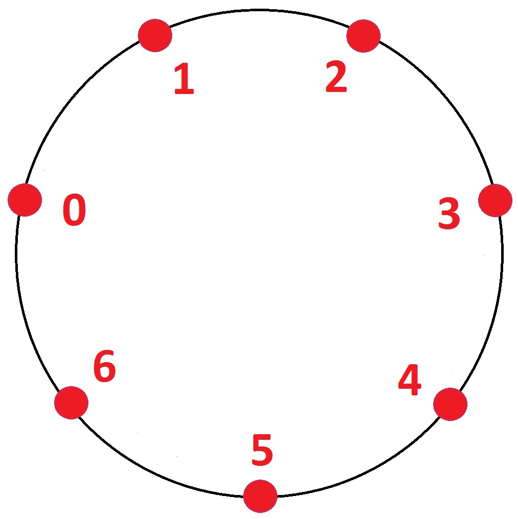
Figure 1: A simple graph with $7$ vertices which approximates a circular one-dimensional space.

$\Delta$ is the length of graph edges. In the continuous limit, $\Delta\rightarrow 0$ (where matricial product turns into a convolution), we obtain

$$\partial\varphi(x) = \lim_{\Delta\rightarrow 0}\frac{1}{2\Delta}\int\tilde{M}(x,y)\varphi(y)dy$$

$$\partial\varphi(x) = \lim_{\Delta\rightarrow 0}\frac{1}{2\Delta}\int\left[\delta(y-(x+\Delta))-\delta(y-(x-\Delta))\right]\varphi(y)dy$$

$$\partial\varphi(x) = \lim_{\Delta\rightarrow 0}\frac{\varphi(x+\Delta)-\varphi(x-\Delta)}{2\Delta}=\partial\varphi(x)$$ (45)

In this way our definition is consistent with the usual definition of derivative.

While increasing the number of points, a $(-1)$ still remains in the up right corner of the matrix, and a $(+1)$ in the down left corner as well. To remove those two non-null terms, it is sufficient to make them unnecessary, by imposing boundary conditions that make the field null in the first and in the last point.

In fact we can describe an open universe (a straight line in one dimension), starting from a closed universe (a circle) and making the radius to tend to infinity. Hence we see that the conditions of null field in the first and in the last point become the traditional boundary conditions for the Standard Model fields.

Remark 1

Note that in spaces with more than one dimension, a derivative matrix $\tilde{M}_{\mu}$ assumes the form (LABEL:forma) only if we number the vertices progressively along the coordinate $\mu$. However, two different numberings can be always related by a vertices permutation.

3 Local translations

In this section we introduce a non-local gauge field for local translations. Moreover we see that such field is enough to describe a covariant quantum theory (ie a quantum theory of gravity).

A global translation for a scalar field $\varphi$ is given by

$$\varphi^{\prime}(x)=\varphi(x+\lambda)=e^{\lambda^{\mu}\partial_{\mu}}\varphi(x).$$

A local translation is then given by

$$\varphi^{\prime}(x)=\varphi(x+\lambda(x))=E(\lambda(x))\varphi(x)$$

where

$$E(\lambda)=1+\lambda^{\mu}\partial_{\mu}+\frac{1}{2!}\lambda^{\mu_{1}}\lambda^{\mu_{2}}\partial_{\mu_{1}}\partial_{\mu_{2}}+\ldots+\frac{1}{n!}\lambda^{\mu_{1}}\ldots\lambda^{\mu_{n}}\partial_{\mu_{1}}\ldots\partial_{\mu_{n}}$$

While for global translations we have $(\partial_{\nu}\varphi)^{\prime}(x)=(\partial_{\nu}\varphi)(x+\lambda)=e^{\lambda^{\mu}\partial_{\mu}}\partial_{\nu}\varphi(x)$, for local translations we have $\partial_{\nu}\varphi^{\prime}(x)=\partial_{\nu}\varphi(x+\lambda(x))\neq E(\lambda)\partial_{\nu}\varphi(x)$. Conversely:

$$\partial_{\nu}\varphi^{\prime}(x)=E(\lambda(x))\partial_{\nu}\varphi(x)+\left[\partial_{\nu},E(\lambda(x))\right]\varphi(x)$$

We take $\partial^{\prime}=\partial$ and $(\partial_{\nu}\varphi)^{\prime}=\partial_{\nu}\varphi^{\prime}$ insofar as translations are considered transformations of fields and not of coordinates. Accepted this we can define a covariant derivative

$$D_{\nu}=\partial_{\nu}+G_{\nu}$$

where $G_{\nu}$ is a gauge field with transformation law

$$G_{\nu}\rightarrow G^{\prime}_{\nu}=E(\lambda)G_{\nu}E^{-1}(\lambda)-\left[\partial_{\nu},E(\lambda)\right]E^{-1}(\lambda).$$

The transformation law for $D$ is easily calculated:

$$(D\varphi)^{\prime} = D^{\prime}_{\nu}\varphi^{\prime}=(\partial^{\prime}_{\nu}+G^{\prime}_{\nu})\varphi^{\prime}=(\partial_{\nu}+G^{\prime}_{\nu})\varphi^{\prime}=$$ (46)

$$= E(\lambda)(\partial_{\nu}\varphi)+\left[\partial_{\nu},E(\lambda)\right]\varphi+E(\lambda)G_{\nu}\varphi-\left[\partial_{\nu},E(\lambda)\right]\varphi=$$

$$= E(\lambda)(\partial_{\nu}+G_{\nu})\varphi=E(\lambda)(D_{\nu}\varphi)$$

Hence

$$D^{\prime}_{\nu}=E(\lambda)D_{\nu}E^{-1}(\lambda)=D_{\nu}$$

What is $E^{-1}(\lambda)$? Consider that

$$\varphi(x)=E^{-1}(\lambda)\varphi^{\prime}(x)=E^{-1}(\lambda)\varphi(x+\lambda(x))$$

Defining a new coordinate $x^{\prime}=x+\lambda(x)$ we obtain

$$\varphi(x^{\prime}-\lambda(x(x^{\prime})))=E^{-1}(\lambda)\varphi(x^{\prime})$$

$$E^{-1}(\lambda)=E(-\lambda^{\prime})$$

$$\quad=1-\lambda^{\mu}\frac{\partial}{\partial x^{\prime\mu}}+\frac{1}{2!}\lambda^{\mu_{1}}\lambda^{\mu_{2}}\frac{\partial}{\partial x^{\prime\mu_{1}}}\frac{\partial}{\partial x^{\prime\mu_{2}}}+\ldots+\frac{(-1)^{n}}{n!}\lambda^{\mu_{1}}\ldots\lambda^{\mu_{n}}\frac{\partial}{\partial x^{\prime\mu_{1}}}\ldots\frac{\partial}{\partial x^{\prime\mu_{n}}}$$

$$\frac{\partial}{\partial x^{\prime\mu}}=\left.\left(\frac{\partial(x+\lambda(x))}{\partial x}\right)^{-1}\right.^{\nu}_{\phantom{a}\mu}\partial_{\nu}$$

What’s about $\varphi^{\prime}(x^{\prime})$ ?

$$\varphi^{\prime}(x^{\prime}) = \varphi^{\prime}(x+\lambda(x))=\varphi(x^{\prime}+\lambda(x^{\prime}))=$$ (47)

$$= \varphi(x+\lambda(x)+\lambda(x+\lambda(x)))=\varphi(x+\Lambda(x))=$$

$$= E(\Lambda(x))\varphi(x)$$

with $\Lambda(x)=\lambda(x)+\lambda(x+\lambda(x))$.

Take now a field $G_{\nu}$ which is pure gauge, explicitly $G_{\nu}=0$. Under a translation $x\rightarrow x+\Lambda(x)$ we have

$$D_{\nu} = \partial_{\nu}$$

$$G^{\prime}_{\nu} = -\left[\partial_{\nu},E(\Lambda)\right]E(-\Lambda^{\prime})$$

$$D^{\prime}_{\nu} = E(\Lambda)\partial_{\nu}E(-\Lambda^{\prime})$$ (48)

$$= \left.\left(\frac{\partial(x+\lambda(x))}{\partial x}\right)^{-1}\right.^{\mu}_{\phantom{a}\nu}\partial_{\mu}=\frac{\partial}{\partial(x+\lambda(x))^{\nu}}=\frac{\partial}{\partial x^{\prime\nu}}$$

The last relation is been obtained in three steps:

$$\partial_{\nu}E(-\Lambda^{\prime})\underbrace{E(\Lambda)\varphi(x)}_{\varphi^{\prime}(x^{\prime})}=\partial_{\nu}\varphi(x)$$

$$E(\Lambda)\partial_{\nu}E(-\Lambda^{\prime})\underbrace{E(\Lambda)\varphi(x)}_{\varphi^{\prime}(x^{\prime})}=E(\Lambda)\partial_{\nu}\varphi(x)$$

$$D^{\prime}_{\nu}\varphi^{\prime}(x^{\prime})=(\partial_{\nu}\varphi)(x+\Lambda(x))=(\partial_{\nu}\varphi)^{\prime}(x+\lambda(x))=\frac{\partial}{\partial x^{\prime\nu}}\varphi^{\prime}(x^{\prime})$$

Note that we have recovered the usual definition of $\partial^{\prime}$, ie

$$\partial^{\prime}_{\nu}=\frac{\partial}{\partial x^{\prime\nu}}=\frac{\partial}{\partial(x+\lambda(x))^{\nu}}$$

We see that the action of a local translation $x\rightarrow x+\Lambda(x)$ corresponds to the diffeomorphism $x\rightarrow x^{\prime}=x+\lambda(x)$ with $\Lambda(x)=\lambda(x)+\lambda(x+\lambda(x))$. Hence we have two choices to obtain invariance under diffeomorphisms:

1. To define $e^{\mu}_{a}(x)$ with $e^{\prime\mu}_{a}(x^{\prime})=\frac{\partial x^{\prime\mu}}{\partial x^{\nu}}e^{\nu}_{a}(x)$, in such a way to have

   $$\mathfrak{S}=\int d^{4}x\,\eta^{ab}e^{\mu}_{a}e^{\nu}_{b}(\partial_{\mu}\varphi)(\partial_{\nu}\varphi)$$

   invariant;

2. To introduce a vector field $G_{\nu}$ which transforms as an ordinary gauge field

   $$G_{\nu}\rightarrow G^{\prime}_{\nu}=E(\Lambda)G_{\nu}E(-\Lambda^{\prime})-\left[\partial_{\nu},E(\Lambda)\right]E(-\Lambda^{\prime})$$

   in such a way to have

   $$\mathfrak{S}=\int d^{4}x\,\eta^{\mu\nu}(D_{\mu}\varphi)(D_{\nu}\varphi)$$

   invariant.

The last case requires a bit of attention. In fact $\mathfrak{S}$ is invariant if and only if the field $\varphi$ transforms according to the rule

$$\varphi(x)\rightarrow\varphi^{\prime}(x^{\prime})=E(\Lambda)\varphi(x)E(-\Lambda^{\prime})$$

instead of

$$\varphi(x)\rightarrow\varphi^{\prime}(x^{\prime})=E(\Lambda)\varphi(x).$$

However $\varphi^{\prime}(x^{\prime})=E(\Lambda)\varphi(x)$ in both cases when it applies to a constant field. Substituting in $\mathfrak{S}$ we find:

$$\mathfrak{S}^{\prime} = \int d^{4}x\,\eta^{\mu\nu}E(\Lambda)(D_{\mu}\varphi)\underbrace{E(-\Lambda^{\prime})E(\Lambda)}_{=1}(D_{\nu}\varphi)E(-\Lambda^{\prime})$$

$$= \int d^{4}x\,\eta^{\mu\nu}E(\Lambda)(D_{\mu}\varphi)(D_{\nu}\varphi)E(-\Lambda^{\prime})$$

In the discrete framework the operators $E$ are simple matrices and $\int d^{4}x$ acts as a trace. Hence we can apply the cyclicity property:

$$\mathfrak{S}^{\prime} = \int d^{4}x\,\eta^{\mu\nu}\underbrace{E(-\Lambda^{\prime})E(\Lambda)}_{=1}(D_{\mu}\varphi)(D_{\nu}\varphi)$$

$$= \int d^{4}x\,\eta^{\mu\nu}(D_{\mu}\varphi)(D_{\nu}\varphi)=\mathfrak{S}$$

Pay attention that $(\partial_{\nu}\varphi)$ is equal to $\partial_{\nu}\varphi-\varphi\partial_{\nu}$ and so it corresponds to $[\tilde{M},\varphi]$ with $\varphi$ in diagonal representation. At the same time the appearance of $E(\Lambda)$ is very simple: it has a $1$ for every $p_{i}$ in the crossing between the row $p_{i}$ and the column $p_{i}+\Lambda(p_{i})$. Other entries are zero. Finally $E(-\Lambda^{\prime})$ is calculated as the inverse of $E(\Lambda)$.

In presence of fields with spin we have to add the usual spin connection $\omega$ in order to compensate local Lorentz transformations. It is necessary because diffeomorphisms cause simultaneously a local shift of coordinates and a local “rotation” of axes. Clearly this last doesn’t affect scalar fields. Putting all together:

$$D_{\mu}=\partial_{\mu}+G_{\mu}+\omega_{\mu}^{ij}\qquad\quad i,j=0,1,2,3\qquad\omega^{ij}=-\omega^{ji}$$

Obviously all fields transform homogeneously under local translations:

$$\overline{\psi} \rightarrow \overline{\psi}^{\prime}=E\overline{\psi}E^{-1}$$

$$\psi \rightarrow \psi^{\prime}=E\psi E^{-1}$$

$$A_{\mu} \rightarrow A^{\prime}_{\mu}=EA_{\mu}E^{-1}$$

$$D_{\mu}\varphi \rightarrow (D_{\mu}\varphi)^{\prime}=E(D_{\mu}\varphi)E^{-1}$$ (49)

We see that all fields can be local only in a specified gauge. In other words, given a local field $\varphi$ in the diagonal representation, its transformed $\varphi^{\prime}=E\varphi E^{-1}$ is highly non local.

4 Ricci scalar and Feynman diagrams

In some gauge the Ricci Scalar is given by

$$R=\alpha\left[(\partial_{\rho}+A_{\rho}),(\partial_{\sigma}+A_{\sigma})\right]\left[G_{\mu},G_{\nu}\right]\eta^{\mu\rho}\eta^{\nu\sigma}\qquad\quad\alpha\in\mathbf{R}$$

However, the covariant combination

$$K=\alpha[D_{\mu},D_{\nu}][D_{\rho},D_{\sigma}]\eta^{\mu\rho}\eta^{\nu\sigma}$$

is equivalent to Ricci scalar plus a topological term (usually called “Gauss-Bonnet term”). Moreover we can extract from $K$ the propagators of $G$ and $A$ as it happens in ordinary gauge theories. Adding the expected fermionic term $\bar{\psi}\gamma^{\mu}D_{\mu}\psi$, the Feynman vertices of quantum gravity are the ones in figure 2.

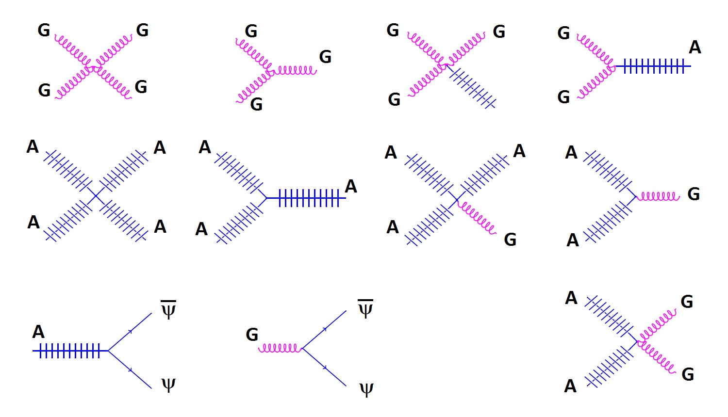
Figure 2: Feynman diagrams in Quantum Gravity.

The price for treating Quantum Gravity as a gauge theory is the inclusion of non-local fields. Explicitly, the path integral must contain not only integrations over diagonal fields $\varphi(x)$, $\psi(x)$ $\bar{\psi}(x)$, $A_{\mu}(x)$ and $G_{\mu}(x)$, but also over non-local fields $\varphi(x,y)$, $\psi(x,y)$ $\bar{\psi}(x,y)$, $A_{\mu}(x,y)$ and $G_{\mu}(x,y)$.

In this way we recover the fundamental result of Arrangement Field Theory, ie that metric appears when locality principle is imposed. Fortunately we can choose a local gauge, which in contrast gives non-local ghost fields.

5 Structure constants

Our target is now the calculation of structure constants for the group of local translations. We start from a gauge field $G_{\mu}$ which is pure gauge:

$$G^{(\alpha)}_{\mu}=-[\partial_{\mu},E(\alpha)]E(-\alpha^{\prime})=-\partial_{\mu}+E(\alpha)\partial_{\mu}E(-\alpha^{\prime})$$

Applying it to $\varphi(x^{\prime})$ with $x^{\prime}=x+\alpha(x)$:

$$G^{(\alpha)}_{\mu}\varphi(x^{\prime}) = -\partial_{\mu}\varphi(x^{\prime})+E(\alpha)\partial_{\mu}\varphi(x)$$

$$= -\frac{\partial x^{\prime\nu}}{\partial x^{\mu}}\frac{\partial}{\partial x^{\prime\nu}}\varphi(x^{\prime})+\frac{\partial}{\partial x^{\prime\mu}}\varphi(x^{\prime})$$

$$= -\frac{\partial}{\partial x^{\prime\mu}}\varphi(x^{\prime})-(\partial_{\mu}\alpha^{\nu}(x))\frac{\partial}{\partial x^{\prime\nu}}\varphi(x^{\prime})+\frac{\partial}{\partial x^{\prime\mu}}\varphi(x^{\prime})$$

$$= -(\partial_{\mu}\alpha^{\nu}(x))\frac{\partial}{\partial x^{\prime\nu}}\varphi(x^{\prime})$$

$$\Longrightarrow G^{(\alpha)}_{\mu} = -\frac{(\partial_{\mu}\alpha^{\nu})}{\left[\delta^{\nu}_{\gamma}+\partial_{\gamma}\alpha^{\nu}\right]}\partial_{\gamma}$$

We can write

$$-\frac{(\partial_{\mu}\alpha^{\nu})}{\left[\delta^{\nu}_{\gamma}+\partial_{\gamma}\alpha^{\nu}\right]}\overset{!}{=}\tilde{\alpha}^{i}_{\mu}f^{\gamma}_{i}(x)$$ (51)

where we have introduced a base of functions $\{f^{\gamma}_{i}(x)\}$ for a suitable Hilbert space and complex constants $\tilde{\alpha}^{i}_{\mu}$. We conclude that a generic $G^{(\alpha)}_{\mu}$ has form $\tilde{\alpha}^{i}_{\mu}f^{\gamma}_{i}(x)$ with $\tilde{\alpha}^{i}_{\mu}$ not restricted by (51). It follows:

$$[G^{(\alpha)}_{\mu},G^{(\beta)}_{\nu}] = \tilde{\alpha}^{i}_{\mu}\tilde{\beta}^{j}_{\nu}(f^{\sigma}_{i}\partial_{\sigma}f^{\gamma}_{j}-f^{\sigma}_{j}\partial_{\sigma}f^{\gamma}_{i})\partial_{\gamma}$$ (52)

$$= \tilde{\alpha}^{i}_{\mu}\tilde{\beta}^{j}_{\nu}\Gamma^{l}_{\phantom{a}ij}f^{\gamma}_{l}\partial_{\gamma}$$

where $\Gamma^{l}_{\phantom{a}ij}$ are structure constants of local translations with

$$\Gamma^{l}_{\phantom{a}ij}=\Big{(}f^{\sigma}_{i}\partial_{\sigma}f^{\gamma}_{j}-f^{\sigma}_{j}\partial_{\sigma}f^{\gamma}_{i}\,\,\,,\,\,\,f^{\gamma}_{l}\Big{)}.$$

Summarizing, local translations define an infinite dimensional non-abelian group with generators $f^{\gamma}_{i}\partial_{\gamma}$ and structure constants $\Gamma^{l}_{\phantom{a}ij}$.

Consider now the commutator between $G^{(\alpha)}_{\mu}$ and the spin-connection $\omega^{ab}_{\nu}(x)=\omega^{abj}_{\nu\tau}f^{\tau}_{j}(x)$:

$$\left[G^{(\alpha)}_{\mu},\omega^{ab}_{\nu}\right]=\tilde{\alpha}^{i}_{\mu}\omega^{abj}_{\nu\tau}E^{l}_{\phantom{a}ij}f^{\tau}_{l}$$

$$E^{l}_{\phantom{a}ij}=\Big{(}f^{\sigma}_{i}\partial_{\sigma}f^{\tau}_{j}\,\,\,,\,\,\,f^{\tau}_{l}\Big{)}.$$

We understand that local Poincaré doesn’t factorize in Lorentz $\times$ translations, due to non-zero structure constants $E^{l}_{\phantom{a}ij}$. Lorentz and translations remain subgroups, but they are no longer independent.

We choose as base functions $f_{i}(x)=\frac{1}{(2\pi)^{2}}\lambda^{(\tau(i))}e^{ip(i)_{\nu}x^{\nu}}$, where $\lambda^{(\tau)}$ is a column array with $1$ in the $\tau$-th entry and $0$ elsewhere $(\lambda^{(\tau)\sigma}=\delta^{\tau\sigma})$. Moreover we impose $(\lambda^{\sigma},\lambda^{\gamma})=\delta^{\sigma\gamma}$. The structure constants result

$$\Gamma^{l}_{\phantom{a}ij} = \int d^{4}x\,\frac{1}{(2\pi)^{6}}\left[\lambda^{(\tau(i))\sigma}e^{ip(i)_{\nu}x^{\nu}}(ip(j)_{\sigma})e^{ip(j)_{\nu}x^{\nu}}(\lambda^{\tau(j)},\lambda^{\tau(l)})\right.-$$

$$\qquad\qquad\quad-\left.\lambda^{(\tau(j))\sigma}e^{ip(j)_{\nu}x^{\nu}}(ip(i)_{\sigma})e^{ip(i)_{\nu}x^{\nu}}(\lambda^{\tau(i)},\lambda^{\tau(l)})\right]e^{-ip(l)_{\nu}x^{\nu}}$$

$$= \int d^{4}x\,\frac{i}{(2\pi)^{6}}(\delta^{\tau(i)\tau(l)}p(j)_{\tau(i)}-\delta^{\tau(j)\tau(l)}p(i)_{\tau(j)})e^{i(p(i)_{\nu}+p(j)_{\nu}-p(l)_{\nu})x^{\nu}}$$

$$= \frac{i}{(2\pi)^{2}}\Big{(}\delta^{\tau(i)\tau(l)}p(j)_{\tau(i)}-\delta^{\tau(j)\tau(l)}p(i)_{\tau(j)}\Big{)}\delta^{4}(p(i)+p(j)-p(l))$$

In the two last lines there is no sum over repeated indices $\tau(i)$ and $\tau(j)$. The $\delta^{4}$ implies the usual momenta conservation in trivalent vertices. More important is to note that $\Gamma\sim p$, while in usual gauge theories we have $\Gamma\sim 1$. Fortunately this defect is compensated by propagator. In fact

$$\text{Kinetic term}\sim(\partial G)^{2}\sim(\partial\tilde{\alpha}\partial)^{2}\sim(p^{2}\tilde{\alpha})^{2}\sim p^{4}\tilde{\alpha}^{2}$$

$$\Rightarrow\text{Propagator}\sim\frac{1}{p^{2}}\cdot\frac{1}{p^{2}}$$

and so the extra $\frac{1}{p^{2}}$ compensates the extra $p$ in structure constants.

6 Conclusion

At this point we have a quantum theory of gravity which resembles ordinary gauge theories. This implies that quantum gravity has the same superficial degree of divergence of gauge theories and then it is apparently quantizable. You just have to try to calculate the first gravitational amplitudes.

References

- [1] Marin, D.: Arrangement Field Theory: beyond Strings and Loop Gravity. LAP LAMBERT Academic Publishing (August 31, 2012)
- [2] De Leo, S., Ducati, G.: Quaternionic differential operators. Journal of Mathematical Physics, Volume 42, pp.2236-2265. ArXiv: math-ph/0005023 (2001).
- [3] Zhang, F.: Quaternions and matrices of quaternions. Linear algebra and its applications, Volume 251 (1997), pp.21-57. Part of this paper was presented at the AMS-MAA joint meeting, San Antonio, January 1993, under the title “Everything about the matrices of quatemions”.
- [4] Farenick, D., R., Pidkowich, B., A., F.: The spectral theorem in quaternions. Linear algebra and its applications, Volume 371 (2003), pp.75 102.
- [5] Hartle, J. B., Hawking, S. W.: Wave function of the universe. Physical Review D (Particles and Fields), Volume 28, Issue 12, 15 December 1983, pp.2960-2975.
- [6] Bochicchio, M.: Quasi BPS Wilson loops, localization of loop equation by homology and exact beta function in the large-N limit of SU(N) Yang-Mills theory. ArXiv: 0809.4662 (2008).
- [7] Minkowski, H., Die Grundgleichungen fur die elektromagnetischen Vorgange in bewegten Korpern. Nachrichten von der Gesellschaft der Wissenschaften zu Gottingen, Mathematisch-Physikalische Klasse, 53-111 (1908).
- [8] Einstein, A., Die Grundlage der allgemeinen Relativitatstheorie. Annalen der Physik, 49, 769-822 (1916).
- [9] Planck, M., Entropy and Temperature of Radiant Heat. Annalen der Physik, 4, 719-37 (1900).
- [10] von Neumann, J., Mathematical Foundations of Quantum Mechanics. Princeton University Press, Princeton (1932).
- [11] Einstein, A., Podolski, B., Rosen, N., Can quantum-mechanical description of physical reality be considered complete? Phys. Rev., 47, 777-780 (1935).
- [12] Einstein, A., Rosen, N., The Particle Problem in the General Theory of Relativity. Phys. Rev., 48, 73-77 (1935).
- [13] Bohm, D., Quantum Theory. Prentice Hall, New York (1951).
- [14] Bell, J.S., On the Einstein-Podolsky-Rosen paradox. Physics, 1, 195-200 (1964).
- [15] Aspect, A., Grangier, P., Roger, G., Experimental realization of Einstein-Podolsky-Rosen-Bohm Gedankenexperiment: a new violation of Bell’s inequalities. Phys. Rev. Lett. 49, 2, 91-94 (1982).
- [16] Penrose, R., Angular Momentum: an approach to combinatorial space-time. Originally appeared in Quantum Theory and Beyond, edited by Ted Bastin, Cambridge University Press, 151-180 (1971).
- [17] LaFave, N.J., A Step Toward Pregeometry I.: Ponzano-Regge Spin Networks and the Origin of Spacetime Structure in Four Dimensions. ArXiv:gr-qc/9310036 (1993).
- [18] Reisenberger, M., Rovelli, C., ’Sum over surfaces’ form of loop quantum gravity. Phys. Rev. D, 56, 3490-3508 (1997).
- [19] Engle, G., Pereira, R., Rovelli, C., Livine, E., LQG vertex with finite Immirzi parameter. Nucl. Phys. B, 799, 136-149 (2008).
- [20] Banks, T., Fischler, W., Shenker, S.H., Susskind, L., M Theory As A Matrix Model: A Conjecture. Phys. Rev. D, 55, 5112-5128 (1997). Available at URL http://arxiv.org/abs/hep-th/9610043 as last accessed on May 19, 2012.
- [21] Garrett Lisi, A., An Exceptionally Simple Theory of Everything. ArXiv:0711.0770 (2007). Available at URL http://arxiv.org/abs/0711.0770 as last accessed on March 29, 2012.
- [22] Nastase, H., Introduction to Supergravity ArXiv:1112.3502 (2011). Available at URL http://arxiv.org/abs/1112.3502 as last accessed on March 29, 2012.
- [23] Maudlin, T., Quantum Non-locality and Relativity. 2nd ed., Blackwell Publishers, Malden (2002).
- [24] Penrose, R., On the Nature of Quantum Geometry. Originally appeared in Wheeler. J.H., Magic Without Magic, edited by J. Klauder, Freeman, San Francisco, 333-354 (1972).