Crumpling transition of the triangular lattice without open edges: effect of a modified folding rule

Abstract

Folding of the triangular lattice in a discrete three-dimensional space is investigated by means of the transfer-matrix method. This model was introduced by Bowick and co-workers as a discretized version of the polymerized membrane in thermal equilibrium. The folding rule (constraint) is incompatible with the periodic-boundary condition, and the simulation has been made under the open-boundary condition. In this paper, we propose a modified constraint, which is compatible with the periodic-boundary condition; technically, the restoration of translational invariance leads to a substantial reduction of the transfer-matrix size. Treating the cluster sizes $L\leq 7$, we analyze the singularities of the crumpling transitions for a wide range of the bending rigidity $K$. We observe a series of the crumpling transitions at $K=0.206(2)$, $-0.32(1)$, and $-0.76(10)$. At each transition point, we estimate the latent heat as $Q=0.356(30)$, $0.08(3)$, and $0.05(5)$, respectively.

I Introduction

At sufficiently low temperatures, the polymerized membrane becomes flattened macroscopically Nelson87 ; see Refs. Nelson89 ; Nelson96 ; Bowick01 for a review. (The constituent molecules of the polymerized membrane have a fixed connectivity, and the in-plane strain is subjected to finite shear moduli. This character is contrastive to that of the fluid membrane Canham70 ; Helfrich73 , which does not support a shear.) The flat phase is characterized by the long-range orientational order of the surface normals. It is rather peculiar that such a continuous (rotational) symmetry is broken spontaneously for such a two-dimensional manifold. To clarify this issue, a good deal of theoretical analyses have been reported so far. However, it is still unclear whether the transition is critical Kantor86 ; Kantor87 ; Baig89 ; Ambjorn89 ; Renken96 ; Harnish96 ; Baig94 ; Bowick96b ; Wheather93 ; Wheater96 ; David88 ; Doussal92 ; Espriu96 or belongs to a discontinuous one with an appreciable latent heat Paczuski88 ; Kownacki02 ; Koibuchi04 . Actually, in numerical simulations, it is not quite obvious to rule out the possibility of a weak-first-order transition Kantor87b ; Kantor87c ; see also Ref. Kownachi09 .

Meanwhile, a discretized version of the polymerized membrane was formulated by Bowick and coworkers Bowick95 ; Cirillo96 ; Bowick97 . To be specific, they considered a sheet of the triangular lattice embedded in a discretized three-dimensional space (face-centered-cubic lattice); see Fig. 9 (a). (Even more simplified folding model, the so-called planar folding, was studied in Refs. Kantor90 ; DiFrancesco94b ; Cirillo96b .) Owing to the discretization, the folding model admits an Ising-spin representation, for which a variety of techniques, such as the mean-field theory and the transfer-matrix method, are applicable. A peculiarity of this Ising magnet is that the spin variables are subjected to a local constraint (folding rule), which is incompatible with the periodic-boundary condition. Because of this difficulty, the open-boundary condition has been implemented so far Bowick95 ; Bowick97 ; Nishiyama04 ; Nishiyama05 . With the full diagonalization method, the finite clusters with the sizes $L\leq 6$ were considered Bowick95 ; Bowick97 . By means of the density-matrix renormalization group (DMRG) White92 ; Peschel99 , the clusters with $L\leq 29$ and $26$ were treated in Refs. Nishiyama04 and Nishiyama05 , respectively. (The results are overviewed afterward.)

In this paper, we modify the local constraint, aiming to implement the periodic-boundary condition, and restore the translation invariance. Technically, the restoration of translation invariance admits a substantial reduction of the transfer-matrix size. Taking the advantage, we treat the sizes up to $L=7$, and analyze the singularities of crumpling transitions in detail.

The cluster-variation method (CVM) (based on the single-hexagon approximation) revealed a rich character of the discrete folding Cirillo96 ; Bowick97 . According to CVM, there appear the totally flat, octahedral, tetrahedral, and piled-up phases, as the bending rigidity $K$ changes from $\infty$ to $-\infty$. Namely, in respective phases, the triangular-lattice sheet crumples up to form a octahedron, a tetrahedron, and a triangular plaquette; see Fig. 3 of Ref. Bowick95 . (This picture is based on a single-hexagon approximation of CVM. Beyond a mean-field level, the thermal undulations may be induced, particularly, in the vicinity of the transition point, disturbing the shape of the crumpled sheet significantly.) More specifically, the crumpling transitions separating these phases are estimated as $K=0.185$, $-0.294$, and $-0.852$; hereafter, we abbreviate the set of parameters as $(0.185,-0.294,-0.852)$. At each transition point, the latent heat is estimated as $(0.229,0.14,0)$; namely, the third transition is continuous according to CVM. On the one hand, the DMRG simulation Nishiyama04 ; Nishiyama05 indicates the transition point $[0.195(2),-0.32(1),-0.76(1)]$ with the latent heat $[0.365(5),0.04(2),0.03(2)]$; the character of the third transition point is still controversial.

The rest of this paper is organized as follows. In Sec. II, we propose a modified folding rule (1); the transfer-matrix formalism Bowick95 is explicated in the Appendix. In Sec. III, we present the numerical results. The singularities of the crumpling transitions are analyzed in detail. In Sec. IV, we present the summary and discussions.

II A modification of the folding rule

In this section, we present a modified folding rule, Eq. (1). As mentioned in the Introduction, the folding rule, enforced by the prefactors in Eq. (13), is too restrictive to adopt the periodic-boundary condition. So far, the numerical simulation has been performed under the open-boundary condition Bowick95 ; Bowick97 ; Nishiyama04 ; Nishiyama05 .

To begin with, we outline the transfer-matrix formalism; an explicit algorithm is presented in the Appendix. According to Ref. Bowick95 , through a dual transformation, the triangular-lattice folding reduces to an Ising model on the hexagonal lattice, Fig. 9 (a). A drawing of a transfer-matrix strip is presented in Fig. 9 (b). A peculiarity of this reduced Ising model is that the spins surrounding each hexagon are subjected to a constraint. (The constraint originates from the folding rule.) To be specific, the prefactors $U_{j}V_{j}(=0,1)$ of the transfer-matrix element (13) restrict the configuration space. As mentioned in the Introduction, this constraint is incompatible with the periodic-boundary condition. (For instance, a cylindrical paper supports a large strain, whereas an open paper is flexible.)

Aiming to restore the translational invariance, we modify the prefactors. We replace Eq. (13) with

$$\frac{1}{L}\sum_{l=1}^{L}(\prod_{j\neq l}U_{j}V_{j})[(1-p)U_{l}V_{l}+p]\exp[-\sum_{k\neq l}H_{k}(K)-H_{l}(K^{\prime})].$$ (1)

Here, the parameter $L$ denotes the system size, and the explicit formulas for the constraint $U_{j}V_{j}$ and the elastic energy $H_{k}(K)$ are shown in the Appendix. As compared with the original form (13), our modified expression (1) has a defect at $l$, where the folding-rule constraint is released. Because the defect is distributing uniformly by the summation $\sum_{l=1}^{L}$ and the normalization factor $1/L$, the translational invariance is maintained. The parameter $K^{\prime}$ describes the local elastic constant at the defect. The probability of the defect is controlled by the parameter $p$; at $p=0$, the original constraint $U_{l}V_{l}$ recovers, whereas at $p=1$, the constraint disappears $U_{l}V_{l}\to 1$. We stress that a single defect does not alter the thermodynamic (bulk) properties. As a byproduct, two tunable parameters $p$ and $K^{\prime}$ are available. The parameters are adjusted to

$$(p,K^{\prime})=(0.7,1.5K).$$ (2)

A justification of this choice is given in Sec. III.2 (Fig. 2).

III Numerical results

In this section, we present the simulation results. We employed the transfer-matrix method (Appendix) with a modified folding rule, Eq. (1). The numerical diagonalization was performed within a subspace specified by the wave number $k=0$ and the parity even. (In a preliminary survey, we confirmed that the dominant-eigenvalue (thermal equilibrium) state belongs to this subspace.) Here, we make use of the spin-inversion symmetry $\sigma_{i},z_{i}\to\pm\sigma_{i},\pm z_{i}$. (This symmetry group originates from the overall rotation of the crumpled triangular-lattice sheet.) We stress that the wave number $k$ makes sense owing to the restoration of the translational invariance (1).

III.1 Crumpling transitions: A preliminary survey

In Fig. 1, we plot the free-energy gap

$$\Delta f=f_{2}-f_{1},$$ (3)

for the bending rigidity $K$. Here, the free energy per unit cell is given by $f_{i}=-\ln\Lambda_{i}/(2L)$ with the (sub)dominant eigenvalue $\Lambda_{1(2)}$ of the transfer matrix. [Here, the unit cell stands for a triangle of the original lattice rather than a hexagon of the dual lattice; see Fig. 9 (a).]

As mentioned in the Introduction, the triangular-lattice sheet becomes crumpled, as the rigidity $K$ changes from $\infty$ to $-\infty$. In Fig. 1, we see a number of signatures of the crumpling transitions around $K\approx 0.2$, $-0.3$, and $-0.8$. (Note that the closure of the excitation gap indicates an onset of phase transition.) On the one hand, the CVM analysis Cirillo96 ; Bowick97 predicts a series of crumpling transitions at $(0.185,-0.294,-0.852)$. The results appear to be consistent with those of Fig. 1, suggesting that the excitation-gap closure indicates a location of the crumpling transition. Detailed analyses of each singularity are made in Sec. III.3 and Sec. III.4.

III.2 Simulation at $p=1$ and $K^{\prime}=0$

As a comparison, we provide a simulation result, setting the defect parameters to $p=1$ and $K^{\prime}=0$ tentatively. This parameter set has an interpretation that a rupture (pair of open edges) distributes uniformly along the transfer-matrix strip. (This situation is an extention of the open-boundary condition, for which the rupture is static.)

In Fig. 2, we present the free-energy gap $\Delta f$ for the bending rigidity $K$; the range of $K$ is the same as that of Fig. 1. The signatures of crumpling transitions in Fig. 2 are less clear, as compared to those of Fig. 1. This result indicates that the choice of the defect parameters affects the finite-size behavior. In the preliminary stage, we surveyed a parameter space of $p$ and $K^{\prime}$, and arrived at a conclusion that the above choice, Eq. (2), is an optimal one. Note that these parameters are the byproduct of the modification of the folding rule, Eq. (1). Here, we make use of these redundant parameters so as to improve the finite-size behavior, aiming to take the thermodynamic limit reliably.

III.3 Crumpling transition in $K>0$: Analysis of the latent heat via the Hamer method

In Sec. III.1, we observed a series of crumpling transitions. In this section, we analyze the singularity of a transition in the $K>0$ side.

To begin with, we determine the transition point. In Fig. 3, an approximate transition point $K_{c}(L)$ is plotted for $1/L^{2}$. Here, the approximate transition point minimizes the free-energy gap

$$\partial_{K}\Delta f|_{K=K_{c}(L)}=0.$$ (4)

The least-squares fit yields an estimate $K_{c}=0.20617(70)$. Similarly, as for $5\leq L\leq 7$, we obtain an estimate $K_{c}=0.20506(99)$. A discrepancy between these results may be an indicator of possible systematic error. The systematic error appears to be comparable to the fitting error. Regarding both errors as the sources of error margin, we obtain

$$K_{c}=0.206(2).$$ (5)

Based on the transition point $K_{c}(L)$, we estimate the amount of latent heat. According to Ref. Hamer83 , the low-lying eigenvectors of the transfer matrix contain information on the latent heat. We explain the underlying idea, and present the scheme explicitly. At the discontinuous (first-order) transition point, the low-lying spectrum of the transfer matrix exhibits a level crossing, and the discontinuity (sudden drop) of the slope reflects a release of the latent heat. However, the finite-size artifact (level repulsion) smears out the singularity. According to Ref. Hamer83 , regarding the low-lying levels as nearly degenerate, one can resort to the perturbation theory of the degenerated case, and calculate the level splitting (discontinuity of slope) explicitly. To be specific, we consider the matrix

$$V=\left(\begin{array}[]{cc}V_{11}&V_{12}\\ V_{21}&V_{22}\end{array}\right),$$ (6)

with $V_{ij}=\langle i|\partial_{K}T|j\rangle$. The matrix $T$ denotes the transfer matrix; namely, the matrix element $\partial_{K}T$ is given by a product of Eq. (13) and Eq. (17) with $K$ dropped. The bases, $|1\rangle$ and $|2\rangle$, are the (nearly degenerate) eigenvectors of $T$ with the eigenvalues $\Lambda_{1,2}$, respectively. The states $\{|i\rangle\}$ are normalized so as to satisfy $\langle i|T|i\rangle=1$. According to the perturbation theory, the eigenvalues of Eq. (6) yield the level-splitting slopes due to $K$. Hence, the latent heat (per unit cell) is given by a product of this discontinuity and the elastic constant

$$Q(L)=|K_{c}(L)|\sqrt{(V_{11}-V_{22})^{2}+4V_{12}V_{21}}\frac{1}{2L},$$ (7)

for the system size $L$.

In Fig. 4, we plot the latent heat (7) for $1/L^{2}$. The least-squares (linear) fit yields an estimate $Q=0.356(12)$ in the thermodynamic limit. Similarly, we obtain $Q=0.3774(93)$ for $5\leq L\leq 7$. Again, the systematic error appears to be comparable to the fitting error. We estimate

$$Q=0.356(30).$$ (8)

This is a good position to address a few remarks. First, the latent heat, Eq. (8), agrees with that of DMRG Nishiyama04 (see the Introduction), whereas the transition point, Eq. (5), lies out of the error margin. This discrepancy may indicate an existence of systematic error as to the determination of $K_{c}$. A peculiarity DiFrancesco94b of this transition is that in the $K>K_{c}$ side, the system becomes completely flattened; namely, there exist no thermal undulations, as if the system is in the low-temperature limit $K\to\infty$. This peculiarity may gives rise to a bias to $K_{c}$. (As a matter of fact, in Ref. Nishiyama04 , a pronounced hysteresis was observed.) On the contrary, we confirmed that the ambiguity of $K_{c}$ does not influence the latent heat $Q$ very much. (Because of this $K_{c}$ independence, the result $Q$ is reliable, as the above-mentioned consistency with DMRG suggests.) In the next section, the remaining two transitions are analyzed in a unified manner. Second, we consider the $1/L^{2}$ extrapolation scheme. The finite-size data converge rapidly to the thermodynamic limit around the first-order transition point, because the correlation length (typical length scale) $\xi$ remains finite. Hence, the dominant system-size corrections should be described by $1/L^{2}$ (rather than $1/L$).

III.4 Crumpling transitions in $K<0$

In this section, we analyze the remaining transitions in the $K<0$ side.

First, we analyze the transition around $K\approx-0.3$. In Fig. 5, we plot the transition point (4) for $1/L^{2}$. The least-squares fit to these data yields an estimate $K_{c}=-0.320(12)$. Similarly, we obtain $K_{c}=-0.316(28)$ for $5\leq L\leq 7$. The systematic error appears to be negligible, as compared to the fitting error. Considering the latter as the source of error margin, we estimate the transition point as

$$K_{c}=-0.32(1).$$ (9)

In Fig. 6, we plot the latent heat (7) for $1/L^{2}$. The least-squares fit yields $Q=0.077(15)$. Similarly, for $5\leq L\leq 7$, we obtain $Q=0.058(28)$. The fitting and systematic errors are comparable. Considering them as the sources of error margin, we estimate the latent heat as

$$Q=0.08(3).$$ (10)

Second, we turn to the analysis of the transition around $K\approx-0.8$. In Fig. 7, we plot the transition point (4) for $1/L^{2}$. The least-squares fit to these data yields an estimate $K_{c}=-0.76(10)$. Similarly, we obtain $K_{c}=-0.72(24)$ for $5\leq L\leq 7$. The fitting error dominates the systematic error. Neglecting the latter, we obtain

$$K_{c}=-0.76(10).$$ (11)

In Fig. 8, we plot the latent heat (7) for $1/L^{2}$. The least-squares fit yields $Q=0.049(51)$. Similarly, for $5\leq L\leq 7$, we obtain $Q=0.01(11)$. Again, the systematic error appears to be negligible. We estimate the latent heat as

$$Q=0.05(5).$$ (12)

Last, we consider a shaky character of Figs. 3-8 (in particular, Figs. 5-8). Such a shaky character is an artifact due to the cluster size. In the preliminary stage, we surveyed the planar folding Kantor90 ; DiFrancesco94b ; Cirillo96b for considerably large system sizes $L\leq 14$; the configuration space of the planar folding is much restricted. As a result, we found that the finite-size behavior is irregular with respect to $L$; this irregularity is an obstacle to making an extrapolation. Roughly speaking, the finite-size behavior is categorized by $L=0$, $1$, and $2$ mod $3$. Although the enlarged configuration space suppresses this irregularity, a slight irregularity for $L=6(=0$ mod $3)$ still remains. A slight bump of Figs. 5 and 7 may be due to this irregularity. Hence, we consider that the deviations (seemingly curved plots) in Figs. 3-8 are not systematic ones. Rather, considering them as a source of errors, we estimate the error margin by making two independent extrapolations for different sets of system sizes.

IV Summary and discussions

We proposed a modified folding rule, Eq. (1), which enables us to simulate the discrete folding without the open edges. By means of the transfer-matrix method, we investigated a series of the crumpling transitions. We estimate the transition point and the latent heat as $[0.206(2),-0.32(1),-0.76(10)]$ and $[0.356(30),0.08(3),0.05(5)]$, respectively. Our result agrees with the preceding CVM and DMRG results. In particular, our result is in quantitative agreement with that of DMRG.

According to Ref. Bowick97 , the third singularity (around $K\approx-0.8$) is so subtle that it could not be captured until $L=8$. On the contrary, our data in Figs. 1 and 7 succeeds in detecting a signature of a crumpling transition even for $4\leq L\leq 7$. As anticipated, the restoration of the translation invariance leads to an improvement of the finite-size behavior.

As mentioned in the Introduction, it is still unclear whether the third transition is continuous Bowick97 or belongs to a weak-first-order transition Nishiyama05 . The present result (12) does not exclude a possibility of a continuous transition. According to Ref. Bowick97 , around $K\approx-0.8$, through a truncation of the configuration space, the discrete folding reduces to a simplified version of the folding model, the so-called planar folding Kantor90 ; DiFrancesco94b ; Cirillo96b , which exhibits a continuous transition in the $K<0$ side. An examination of this truncation process may provide valuable information on the nature of this phase transition. This problem will be addressed in the future study.

*

Appendix A Transfer-matrix formalism for the discrete folding

In this Appendix, we present the transfer-matrix formalism for the discrete folding Bowick95 . Before commencing a mathematical description, we explicate a basic feature of the discrete folding. We consider a sheet of the triangular lattice, Fig. 9 (a). Along the edges, the sheet folds up. The fold angle $\theta$ along the edges is discretized into four possibilities, namely, “no fold” ($\theta=\pi$), “complete fold” ($\theta=0$), “acute fold” [$\theta={\rm arccos}(1/3)$], and “obtuse fold” [$\theta={\rm arccos}(-1/3)$]; in other words, the triangular lattice is embedded in the face-centered-cubic lattice Bowick95 .

The above discretization leads to an Ising-spin representation. The mapping, the so-called gauge rule, reads as follows Bowick95 . We place two types of Ising variables $\{\sigma_{i},z_{i}\}$ at each triangle $i$ (rather than each joint); see Fig. 9 (a). Hence, hereafter, we consider the a spin model on the dual (hexagonal) lattice. The gauge rule sets the joint angle between the adjacent triangles. That is, provided that the $z$ spins are antiparallel ($z_{1}z_{2}=-1$) for a pair of adjacent neighbors, the joint angle is either an acute or obtuse fold. Similarly, if $\sigma_{1}\sigma_{2}=-1$ folds, the relative angle is either a complete or obtuse fold. The spins are subjected to a constraint (folding rule); The prefactors $U_{j}V_{j}$ of the transfer-matrix element (13) enforces the constraint.

As a consequence, the discrete folding reduces to a two-component Ising model on the hexagon lattice. Hence, the transfer-matrix strip looks like that drawn in Fig. 9 (b). The row-to-row statistical weight $T_{\{\sigma_{i},z_{i}\},\{\sigma^{\prime}_{i},z^{\prime}_{i}\}}$ yields the transfer-matrix element. The transfer-matrix element for the strip width $L$ is given by Bowick95

$$T_{\{z_{i},\sigma_{i}\},\{z^{\prime}_{i},\sigma^{\prime}_{i}\}}=(\prod_{j=1}^{L}U_{j}V_{j})\exp(-H/T),$$ (13)

with

$$U_{j}=\delta(\sigma_{2j-2}+\sigma_{2j-1}+\sigma_{2j}+\sigma^{\prime}_{2j-1}+\sigma^{\prime}_{2j}+\sigma^{\prime}_{2j+1}\ mod\ 3,0),$$ (14)

and

$$V_{j}=\prod_{c=1}^{2}\delta(\alpha_{c}(z_{2j},z_{2j-1},z_{2j-2},z^{\prime}_{2j-1},z^{\prime}_{2j},z^{\prime}_{2j+1})\ mod\ 2,0).$$ (15)

The factors $\{U_{j},V_{j}\}$ enforce the constraint (folding rule) as to the spins surrounding each hexagon. Here, $\delta(m,n)$ denotes Kronecker’s symbol, and $\alpha_{c}$ is given by

$$\alpha_{c}(z_{1},\dots,z_{6})=\sum_{i=1}^{6}\frac{1}{2}(1-z_{i}z_{i+1})\delta(\sum_{j=1}^{i}\sigma_{j}\ mod\ 3,0).$$ (16)

The Boltzmann factor $\exp(-H/T)$ is due to the bending-energy cost $H$. Hereafter, we choose the temperature $T$ as a unit of energy; namely, we set $T=1$. As usual, the bending energy is given by the inner product $\cos\theta_{ij}$ of the surface normals of adjacent triangles. Hence, the bending energy is given by a compact formula

$$H=\sum_{k}H_{k}(K).$$ (17)

Here, the index $k$ specifies each hexagon as in Eq. (13). The local energy of each hexagon $H_{k}$ is given by

$$H_{k}(K)=-0.5\sum_{i=1}^{6}K\cos\theta_{i,i+1}=-0.5\sum_{i=1}^{6}\frac{1}{3}K\sigma_{i}\sigma_{i+1}(1+2z_{i}z_{i+1}),$$ (18)

with the bending rigidity $K$. Here, the summation $\sum_{i=1}^{6}$ runs over all vertices around the hexagon $k$. (The overall factor $0.5$ compensates the duplicated sum.)

Figure 1: The free-energy gap (3) is plotted for the bending rigidity $K$ and the system size $L=$($+$) 4, ($\times$) 5, ($*$) 6, and ($\Box$) 7. The data indicate singularities (crumpling transitions) around $K\approx 0.2$, $-0.3$, and $-0.8$; detailed analyses of each transition are made in Figs. 3-8.

Figure 2: The free-energy gap (3) is plotted for the bending rigidity $K$ and the system size $L=$($+$) 4, ($\times$) 5, ($*$) 6, and ($\Box$) 7. Tentatively, the defect parameters [Eq. (1)] are set to $p=1$ and $K^{\prime}=0$. The data appear to be scattered, as compared to those of Fig. 1. This result indicates that the finite-size behavior is improved by adjusting the defect parameters.

Figure 3: The crumpling transition $K\approx 0.2$ observed in Fig. 1 is analyzed in detail. The transition point $K_{c}(L)$ (4) is plotted for $1/L^{2}$. The least-squares fit yields an estimate $K_{c}=0.20617(70)$.

Figure 4: The latent heat $Q(L)$ (7) is plotted for $1/L^{2}$. The least-squares fit yields an estimate $Q=0.356(12)$.

Figure 5: The crumpling transition $K\approx-0.3$ observed in Fig. 1 is analyzed in detail. The transition point $K_{c}(L)$ (4) is plotted for $1/L^{2}$. The least-squares fit yields an estimate $K_{c}=-0.320(12)$.

Figure 6: The latent heat $Q(L)$ (7) is plotted for $1/L^{2}$. The least-squares fit yields an estimate $Q=0.077(15)$.

Figure 7: The crumpling transition $K\approx-0.8$ observed in Fig. 1 is analyzed in detail. The transition point $K_{c}(L)$ (4) is plotted for $1/L^{2}$. The least-squares fit yields an estimate $K_{c}=-0.76(10)$.

Figure 8: The latent heat $Q(L)$ (7) is plotted for $1/L^{2}$. The least-squares fit yields an estimate $Q=0.049(51)$.

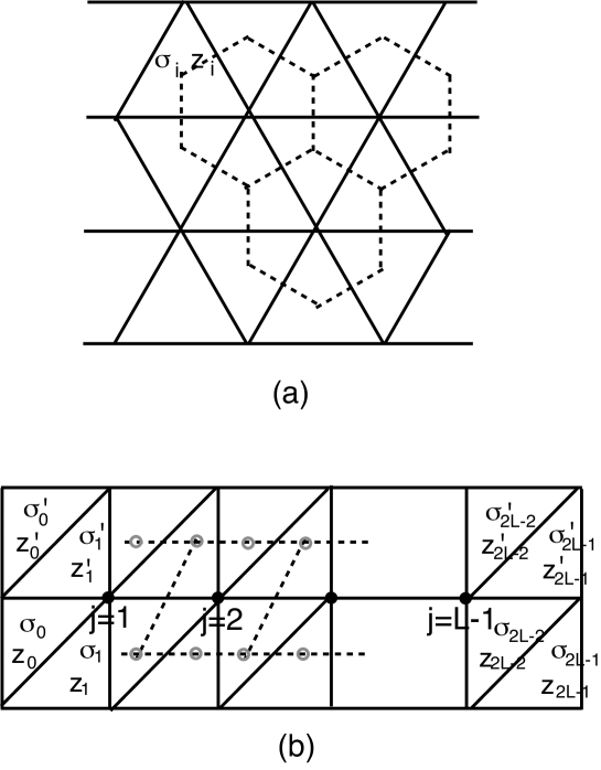
Figure 9: (a) We consider a discrete folding of the triangular lattice. In order to specify the fold angle, we place two types of Ising variables $\{z_{i},\sigma_{i}\}$ on each triangle $i$ rather than at each joint (gauge rule Bowick95 ). Hence, hereafter, we consider a spin model on the dual (hexagonal) lattice. (b) Construction of the transfer matrix. The row-to-row statistical weight yields the transfer-matrix element, Eq. (13). So far, the open-boundary condition has been imposed. Here, we restore the translational invariance by using a modified folding rule (1).

References

- (1) D. R. Nelson and L. Peliti, J. Phys. (France) 48, 1085 (1987).
- (2) D. Nelson, T. Piran and S. Weinberg, Statistical Mechanics of Membranes and Surfaces, Volume 5 of the Jerusalem Winter School for Theoretical Physics (World Scientific, Singapore, 1989).
- (3) P. Ginsparg, F. David and J. Zinn-Justin, Fluctuating Geometries in Statistical Mechanics and Field Theory (Elsevier Science, The Netherlands, 1996).
- (4) M. J. Bowick and A. Travesset, Phys. Rep. 344, 255 (2001).
- (5) P. Canham, J. Theor. Biol. 26, 61 (1970).
- (6) W. Helfrich, Z. Naturforsch. C 28, 693 (1973).
- (7) Y. Kantor, M. Kardar and D. R. Nelson, Phys. Rev. Lett. 57, 791 (1986).
- (8) Y. Kantor, M. Kardar and D. R. Nelson, Phys. Rev. A 35, 3056 (1987).
- (9) M. Baig, D. Espriu and J. Wheater, Nucl. Phys. B 314, 587 (1989).
- (10) J. Ambjørn, B. Durhuus and T. Jonsson, Nucl. Phys. B 316, 526 (1989).
- (11) R. Renken and J. Kogut, Nucl. Phys. B 342, 753 (1990).
- (12) R. Harnish and J. Wheater, Nucl. Phys. B 350, 861 (1991).
- (13) M. Baig, D. Espiu and A. Travesset, Nucl. Phys. B 426, 575 (1994).
- (14) M. Bowick, S. Catterall, M. Falcioni, G. Thorleifsson and K. Anagnostopoulos, J. Phys. I (France) 6, 1321 (1996).
- (15) J. F. Wheater and P. Stephenson, Phys. Lett. B 302, 447 (1993).
- (16) J. F. Wheater, Nucl. Phys. B 458, 671 (1996).
- (17) F. David and E. Guitter, Europhys. Lett. 5, 709 (1988).
- (18) P. Le Doussal and L. Radzihovsky, Phys. Rev. Lett. 69, 1209 (1992).
- (19) D. Espriu and A. Travesset, Nucl. Phys. B 468, 514 (1996).
- (20) M. Paczuski, M. Kardar and D. R. Nelson, Phys. Rev. Lett. 60, 2638 (1988).
- (21) J.-Ph. Kownacki and H. T. Diep, Phys. Rev. E 66, 066105 (2002).
- (22) H. Koibuchi, N. Kusano, A. Nidaira, K. Suzuki, and M. Yamada, Phys. Rev. E 69, 066139 (2004).
- (23) Y. Kantor and D. R. Nelson, Phys. Rev. Lett. 58, 2774 (1987).
- (24) Y. Kantor and D. R. Nelson, Phys. Rev. A 36, 4020 (1987).
- (25) J.-P. Kownacki and D. Mouhanna, Phys. Rev. E 79, 040101(R) (2009).
- (26) M. Bowick, P. Di Francesco, O. Golinelli and E. Guitter, Nucl. Phys. B 450, 463 (1995).
- (27) E. Cirillo, G. Gonnella and A. Pelizzola, Phys. Rev. E 53, 3253 (1996).
- (28) M. Bowick, O. Golinelli, E. Guitter and S. Mori, Nucl. Phys. B 495, 583 (1997).
- (29) Y. Kantor and M. V. Jarić, Europhys. Lett. 11, 157 (1990).
- (30) P. Di Francesco and E. Guitter, Phys. Rev. E 50, 4418 (1994).
- (31) E. N. M. Cirillo, G. Gonnella and A. Pelizzola, Phys. Rev. E 53, 1479 (1996).
- (32) Y. Nishiyama, Phys. Rev. E 70, 016101 (2004).
- (33) Y. Nishiyama, Phys. Rev. E 72, 036104 (2005).
- (34) S. R. White, Phys. Rev. Lett. 69, 2863 (1992).
- (35) I. Peschel, X. Wang, M. Kaulke and K. Hallberg, Density-Matrix Renormalization: A New Numerical Method in Physics (Springer-Verlag, Berlin, 1999).
- (36) C.J. Hamer, J. Phys. A 16, 3085 (1983).