Active Matter
Gautam I. Menon
The Institute of Mathematical Sciences
CIT Campus, Taramani, Chennai 600 113 INDIA
Abstract
The term active matter describes diverse systems, spanning macroscopic (e.g. shoals of fish and flocks of birds) to microscopic scales (e.g. migrating cells, motile bacteria and gels formed through the interaction of nanoscale molecular motors with cytoskeletal filaments within cells). Such systems are often idealizable in terms of collections of individual units, referred to as active particles or self-propelled particles, which take energy from an internal replenishable energy depot or ambient medium and transduce it into useful work performed on the environment, in addition to dissipating a fraction of this energy into heat. These individual units may interact both directly as well as through disturbances propagated via the medium in which they are immersed. Active particles can exhibit remarkable collective behaviour as a consequence of these interactions, including non-equilibrium phase transitions between novel dynamical phases, large fluctuations violating expectations from the central limit theorem and substantial robustness against the disordering effects of thermal fluctuations. In this chapter, following a brief summary of experimental systems which may be classified as examples of active matter, I describe some of the principles which underlie the modeling of such systems.
1 Introduction to Active Fluids
Anyone who has admired the intricate dynamics of a group of birds in flight or the coordinated, almost balletic maneuvers of a school of swimming fish can appreciate the motivation for the study of “active matter”: How do individual self-driven units, such as wildebeest, starlings, fish or bacteria, flock together, generating large-scale, spatiotemporally complex dynamical patterns [51]? What are the rules which govern this dynamics and how do the principles of physics constrain the behaviour of each such unit? Finally, what are the simplest possible models for such behaviour and is there any commonality to the description of these varied problems [46, 47, 48]?
Describing these diverse problems in terms of individual “agents” which evolve via a basic set of update rules while interacting with other agents provides a general way of approaching a large number of unrelated problems. These include the description of the propagation of infectious diseases in a population, the seasonal migration of animal populations, the collective motion and coordinated activities of groups of ants and bees and the swimming of shoals of fish [48]. Of these problems, the subset of problems involving agents whose mechanical behaviour at a scale larger than the individual agent must be constrained by local conservation laws, such as the conservation of momentum, forms a special class [44]. It is these systems that are the primary focus of this chapter.
Generalizing from the examples above, a tentative definition of active matter might be the following: Active matter is a term which describes a material (either in the continuum or naturally decomposable into discrete units), which is driven out of equilibrium through the transduction of energy derived from an internal energy depot or ambient medium into work performed on the environment. Such systems are generically capable of emergent behaviour at large scales. The hydrodynamic description of such problems should be equally applicable to situations where the granularity of the constituent units is not resolved, but which are rendered non-equilibrium in a qualitatively similar way [48, 39].
What differentiates active systems from other classes of driven systems (sheared fluids, sedimenting colloids, driven vortex lattices etc.) is that the energy input is internal to the medium (i.e. located on each unit) and does not act at the boundaries or via external fields. Further, the direction in which each unit moves is dictated by the state of the particle and not by the direction imposed by an external field.
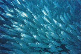
Such individual units are, in general, anisotropic, as in Fig. 1. Collections of such units are thus capable of exhibiting orientationally ordered states. A canonical example of an ordered state of orientable units obtained in thermal equilibrium is the nematic liquid crystal, in which anisotropic particles align along a common axis. Active systems of such units can, in addition, exhibit directed motion along this axis; a concrete example is illustrated in Fig. 1. In the context of active particles in a fluid, the terminology “swimmers” or “self-propelled particles” is often used, while the terms “active nematic” or “living liquid crystals” occur in the discussion of the orientationally ordered collective states of active particles [39].
Why study active systems? For one, such systems can display phases and phase transitions absent in systems in thermal equilibrium [46, 47]. For another, active matter often exhibits unusual mechanical properties, including strong instabilities of ordered states to small fluctuations. Such instabilities may be generic in the sense that they should appear in any hydrodynamic theory which enforces momentum conservation and includes the lowest order contribution to the system stress tensor arising from activity [44]. Fluctuations in active systems are generically large, often deviating qualitatively from the predictions of simple arguments based on the central limit theorem [45, 46, 47, 37]. In common with a large number of related non-equilibrium systems, some examples of active matter appear to be self-tuned to the vicinity of a phase transition, where response can be anomalously large and fluctuations dominate the average behaviour.
The study of active matter spans many scales. The smallest scales involve the modeling of individual motile organisms, such as fish or individual bacteria or even nanometer-scale motor proteins such as kinesin or dyneins which move in a directed manner along cytoskeletal filaments. Hydrodynamic descriptions of large numbers of motile organisms operate at a larger length scale, averaged over a number of such swimmers that is large enough for the granularity at the level of the individual swimmer to be neglected, while still allowing for the possibility of spatial fluctuations at an intermediate scale.
Finally, all living matter is matter out of thermodynamic equilibrium. The source of this non-equilibrium is, typically, the hydrolysis of a NTP (nucleoside tri-phosphate, such as ATP or GTP) molecule into its di-phosphate form, releasing energy. This energy release can drive conformational changes in a protein, leading to mechanical work. Biological matter is thus generically internally driven, precisely as demanded by our definition of active matter. Understanding the general principles which govern active matter systems could thus provide ideas, terminology and a consistent set of methods for the modeling of the mechanical behaviour of living, as opposed to dead, biological matter. This is perhaps the most substantial motivation for the study of active matter.
The outline of this chapter is the following: Section 2 provides some examples of matter which can be classified as active, using our definition. Section 3 summarizes results on a simple model for an individual swimmer and summarizes necessary ingredients for a coarse-grained description of a large number of swimmers. Section 4 begins by illustrating the derivation of the equations of motion and the stress tensor of a simple fluid and then goes on to illustrate how this derivation may be extended to describe fluids with orientational order close to thermal equilibrium. It then goes on to discuss how novel contributions to the fluid stress tensor can arise from active fluctuations, deriving an equation of motion for small fluctuations above a pre-assumed nematic state. These calculations lead to predictions for the rheological behaviour of active systems and the demonstration of the instability of the ordered nematic (or polar) state to small fluctuations. In Sect. 5, the theory of active gels is summarized briefly and some results from this formalism are outlined. Section 6 provides a brief summary.
2 Active Matter Systems: Some Examples
The subsections below list a (non-exhaustive) set of examples of active matter systems. The large-scale behaviour of some of these systems is the focus of later sections.
2.1 Dynamical Behaviour in Bacterial Suspensions
Dombrowski et.al. study the velocity fields induced by bacterial motion at the bottom of sessile and pendant drops containing the bacterium B. subtilis [12]. These flows reflect the interplay between bacterial chemotaxis and buoyancy effects which together act to carry bioconvective plumes down a slanted meniscus, concentrating cells at the drop edge (sessile) or at the drop bottom (pendant). The motion exhibited by groups of bacteria as a result of this self-concentration is large-scale at the level of individual bacteria, exhibiting vortical structures and other complex patterns as a consequence of the hydrodynamic interaction between swimming bacteria. Thus, these experiments highlight the crucial role of hydrodynamics, coupled with the motion of individual active swimmers, in generating self-organized, large-scale dynamical fluctuations in the surrounding fluid.
2.2 Mixtures of Cytoskeletal Filaments and Molecular Motors
The influential experiments of Nedelec and collaborators combine a limited number of cytoskeletal and motor elements – microtubules, kinesin complexes and ATP – in a two-dimensional geometry in vitro finding remarkable self-organized patterns evolving from initially disordered configurations [32]. These include individual asters and vortices as well as disordered arrangements of such structures, in addition to bundles and disordered states at varying values of motor densities. These are self-organized structures, large on the scale of the individual cytoskeletal filament and motor, which require ATP (and thus are non-equilibrium) in order to form and be sustained. Several hydrodynamical approaches to this problem have been proposed, as in Ref. [23, 41, 2]. These experiments and associated theory are summarized in Ref. [18].
2.3 Layers of Vibrated Granular Rods
The experiments of Narayanan et.al. take elongated rod-like copper particles in a quasi-two-dimensional geometry, and vibrate them vertically in a shaker [31]. This agitated monolayer of particles is maintained out of equilibrium by the shaking, which effectively acts to convert vertical motion into horizontal motion via the tilting of the rod. The particles are back–front symmetric, and are thus nematic in character. These experiments see large, dynamical regions which appear to fluctuate coherently. Similar behaviour is predicted in theories of flocking behaviour induced purely by increasing the concentration in dense aggregates of particles held out of equilibrium [51, 48]. These experiments provide a particularly striking signature of non-equilibrium steady state behaviour in “flocking” systems: the presence of number fluctuations in such systems which scale anomalously with the size of the region being averaged, i.e., with a power of which exceeds the central limit prediction of a behaviour of number fluctuations [48].
2.4 Fish Schools
Experiments of Makris and collaborators use remote sensing methods on a continental scale to access the structure and dynamics of large-scale shoals of fish, containing an order of a few million individuals [25]. Apart from the relatively rapid time-scale for the reorganization of the shoal – around 1–10 min in their experiments – these experiments also see evidence for “fish waves”; propagating internal disturbances within the shoal which occur at relatively regular intervals, representing disturbances at scales far larger than that of the individual fish. The speeds of such waves are larger, by around a factor of 10, than the velocities of the swimming fish. They appear to represent “locally interconnected compaction events” similar to the Mexican waves exhibited through the coordinated motion of spectators in stadia. It is interesting that similar wave-like excitations are predicted in the hydrodynamic theories of Refs. [47, 44], where they involve waves of concentration and splay [47] or splay–concentration and bend [44].
2.5 Bird Flocks
The STARFLAG collaboration has imaged large flocks of starlings (between and individuals at a time), using computer-aided imaging techniques to understand the dynamics of individual birds and how this dynamics is influenced by the spatial distribution and behaviour of neighbouring birds. Surprisingly, and contrary to what might have been naively expected, birds appear to adjust to the motion of the flock by measuring the behaviour of topologically (and not metrically) related neighbours [3]. Thus, at each instant, each bird appears to be comparing its instantaneous position and velocity to those of the 5–7 birds closest to it, making the adjustments required to maintain the coherence of the flock. This strategy appears to have the advantage that reducing the density of the flock should not then impact the coherence of the flock, since only topological and not metrical relationships are involved, a fact that calls into question the gradient expansions favoured by most theoretical work which represents flocking behaviour by coarse-grained equations of motion for a few hydrodynamic fields.
2.6 Marching Behaviour of Ants and Locusts
Ian Couzin’s group at Princeton has investigated the transition to marching behaviour in locusts. Swarms of the desert locust, Schistocerca gregaria, in their non-flying form, can exist in a relatively solitary individualistic state as well as a gregarious collective state. In the “gregarious” state, such locusts can form huge collective marching units which forage all vegetation in their path. This has a huge social and economic impact on humans, affecting the livelihood of one in ten people on the planet in plague years. These experiments provide an experimental example of the collective transition in simple computational models of flocking behaviour. From more recent work from this group, it appears, somewhat unusually, that the transition is induced by “cannibalistic” behaviour, in which a locust is successful in biting the rear-quarters of the locust immediately in front [7, 10].
2.7 Listeria monocytogenes Motility
The bacterium Listeria monocytogenes is a simple model system for cell motility, which derives its ability to move from the polymerization of actin, leading to the formation of a “comet tail” emerging from the rear of the bacterium [35]. Motility appears to arise from the deformation of the gel formed by the actin and cross-linking proteins as a consequence of continuing polymerization, which results in a propulsive force on the bacterium. The non-equilibrium comes from ATP-driven actin polymerization. Interestingly, many features of the experiment can be reproduced in in vitro systems where actin polymerization is initiated at the surface of specially treated beads, which then exhibit symmetry-breaking motility [29].
2.8 Cell Crawling
There is a vast and intriguing literature on cell crawling on substrates [8, 9, 14, 50]. Such crawling appears to have four basic steps: the extension of cellular protrusions, the attachment to the substrate at the leading edge, the translocation of the cell body and the detachment at the rear. Cell crawling appears to be largely mediated by a meshwork of actin in gel form, whose fluidity is actively maintained through the action of myosin motors and other associated proteins [8, 50]. Interestingly, motility has also been observed in nucleus-lacking cell fragments excised by lasers, over a period of several hours.
2.9 Active Membranes
Experiments on fluctuating giant vesicles containing bacteriorhodopsin (BR) pumps reconstituted in a lipid bilayer indicate that the light-driven proton pumping activity of BR amplifies membrane shape fluctuations[26, 27]. The BR pumps transfer protons in one direction across the membrane as they change conformation upon excitation by light of a specific wavelength. These experiments have been described in terms of a non-equilibrium “active” temperature[26, 27]. Hydrodynamic theories which interpret the experiments via a description of a membrane with a density of embedded diffusing dipolar force centres, i.e. as an “active membrane”, have also been studied in some detail. It is interesting that several developments in the theoretical description of generic active matter reflect ideas first introduced in the context of active membranes[33, 38, 42]. A detailed study of a biologically relevant model of an active membrane system which contains a large number of references to the literature is available in Ref. [21].
3 The Swimmer: Individual and Collective
The examples provided in the previous section are indicative of some of the diversity exhibited by systems which fall under the general category of active matter. These can broadly be classified into systems in which the role of mechanical conservation laws (e.g. for momentum) are important and systems in which, typically, only the conservation of number is relevant.
The flocking model of Vicsek and collaborators [51], recast in terms of hydrodynamic equations of motion by Toner and Tu [46, 47, 48], is an agent-based model in which cooperativity is driven by a density dependent interaction which tends to orient individual units in the direction in which their neighbours move. The environment – the ground and vegetation for the moving locusts, for example, provides merely the background in this case and has no other dynamical significance. In the case of the flock of starlings the communication between individual starlings does not appear to be primarily via the medium, but through visual contact.
The case of the motile bacterium and the swimming fish, on the other hand, are cases where the medium plays an important role in transferring momentum to and from the swimmers and in determining the interactions between swimmers. This case will be discussed below, first for the situation of the individual swimmer and then for collections of swimmers, modeled via a hydrodynamic approach.
3.1 The Individual Swimmer
The central idea in the modeling of individual swimmers is that the system must be force-free, when averaged over lengthscales larger than the characteristic dimension of the swimmer [39, 6]. This is a consequence of Newton’s third law, which imposes that the force exerted by the swimmer on the fluid must be equal and opposite to the force exerted by the fluid on the swimmer. Thus, if one considers the swimmer as a source of forces locally within the fluid which act upon the fluid, such a source cannot have a monopole component but may have a dipole (or higher multipole) component.
Depending on the character of the swimmer, more distinctions are possible [6, 39]. Contractile swimmers or pullers (such as bacteria propelled by flagella at the head of the organism) pull fluid in along the long axis and push it out along an axis normal to their midpoint. Tensile swimmers or pushers push fluid out along their long axis and pull fluid in along the midpoints. They are propelled from the rear, justifying the terminology of pushers.
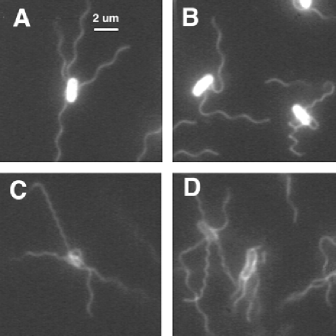
Consider a simple model for a microscopic swimmer. In the Stokes limit, time does not enter these equations explicitly and the velocity field is completely specified by the boundary conditions imposed on the flow. (The use of the Stokes limit is generically justified in the case of bacteria, where characteristic Reynolds numbers at the scale of a single particle are of the order of or smaller.) Reversing the velocity field at the boundaries should retrace the velocity field configuration, implying that the trajectory assumed by the swimmer in its configuration space cannot be time-reversal invariant. The helical or “corkscrew-like” motion of the flagellae of the bacterium E. coli (see Fig. 2), discussed by Purcell [34], provides a particularly attractive example of how the limitations on directed motion at the low Reynolds numbers required for the Stokes limit approximated to be valid can be overcome.
Averaging over multiple strokes of the swimmer simplifies the description: the broken temporal symmetry required for translation in a flow governed by the Stokes equations can be replaced by a broken spatial symmetry. This singles out the direction of motion of the swimmer. Following a model introduced recently by Baskaran and Marchetti (whose notations and treatment we follow closely in this section), the swimmer is modeled as an asymmetric, rigid dumbbell [6]. This dumbbell consists of two differently sized spheres, of radii (large) and (small), forming the head and the tail of the swimmer. The length of the swimmer is the length between the two centers. The orientation of the swimmer is given by the unit vector , drawn from the smaller sphere to the larger sphere.
Thus, the equations of motion of the two spheres, with locations and , are given by
| (1) |
where the constant length between the two spheres is imposed by the constraint that and the velocity field is given by . The no-slip condition at the surfaces of the spheres requires that the sphere move with the velocity of the fluid next to it.
The velocity field obeys the Stokes equation and is constrained by incompressibility,
| (2) |
where the “force” terms which enter on the right hand side are composed of a term which is associated purely with activity (i.e. vanishes in thermal equilibrium) as well as of a second “noise” term modeling the fluctuations in fluid velocity arising from purely thermal fluctuations. Such noise terms do not conventionally enter the Navier-Stokes equations, but must generically be included in a coarse-grained description. Detailed expressions for these forces are available in Ref. [6].
To solve the Stokes equations, we insert a delta function force on the right hand side, representing a fundamental source term from which more complex force configurations can be constructed. In Fourier space, the incompressibility condition is imposed as , while the Stokes equations are . This then gives
| (3) |
with
| (4) |
These are inverted by
| (5) |
The symbol is the unit tensor. In a Cartesian basis of it is
| (6) |
The quantity acting on the force on the right hand side is the Oseen tensor, defined through
| (7) |
for , with a unit vector. The Stokes equations are solved by the superposition
| (8) |
The divergence at short distances is eliminated through the definition: , where .
The dynamics of an extended body in Stokes flow follows from translation of the hydrodynamic centre and rotations about the hydrodynamic centre. (The hydrodynamic centre refers to the point about which the net hydrodynamic torque on the body vanishes; it thus plays the same role in Stokes flow as the centre of mass in inertial dynamics.) For the problem of a rigid dumbbell in an external flow, the hydrodynamic centre is obtained from
| (9) |
The equations of motion for the translation and rotation of the hydrodynamic centre follow from
| (10) |
where the angular velocity describing rotations about the hydrodynamic centre is defined by
| (11) |
and
| (12) |
The random forces and lead to diffusion at large length scales [6].
The forces and the torques arise from hydrodynamic couplings between swimmers. An isolated swimmer is propelled at speed
| (13) |
with velocity . This velocity arises purely as a consequence of the fact that the hydrodynamic and the geometric centers do not coincide. For symmetric swimmers, this velocity is zero and the swimmer is a “shaker” as opposed to a “mover”.
The interactions between swimmers can be calculated in the dilute limit by a multipole expansion, yielding
| (14) |
for the hydrodynamic force exerted by the th swimmer on the th one. In addition, expressions for the hydrodynamic torque between swimmers in the dilute limit can be derived and are presented in Ref. [6].
The hydrodynamic force decays as , as follows from its dipole character. The torque consists of two terms: One is nonzero even for shakers and aligns swimmers regardless of their polarity. The second term vanishes for symmetric swimmers, serving to align swimmers of the same polarity. A more detailed discussion of the structure of the forces and torques for pushers and pullers is available in Ref. [6].
3.2 Multiple Swimmers
The coarse-grained version of the many swimmer problem is defined through the following local fields[4, 5]. First, we must have a density of active particles, defined microscopically in terms of
| (15) |
Second, in the case in which the axes of a fore–aft asymmetric swimmer are largely aligned along a common direction – as in a magnet – we can define a local field describing polar order in the following way:
| (16) |
Third, and finally, when one considers ensembles of interacting swimmers, we must also consider the possibility of additional and more subtle macroscopic variables representing orientational order. An ensemble of individual particles, each aligned, on average, along a common axis, is familiar in soft condensed matter physics. Such systems are referred to as nematics and the ordering as nematic ordering. In such nematic order, the alignment is along a common axis but a vectorial direction is not picked out.
Orientational order in the nematic phase is generally described by a second-rank, symmetric traceless tensor , defined in terms of the second moment of the microscopic orientational distribution function. This (order-parameter) tensor can be expanded as
| (17) |
The three principal axes of this tensor, obtained by diagonalizing in a local frame, specify the direction of nematic ordering , the codirector and the joint normal to these, labeled by . The principal values and represent the strength of ordering in the direction of and , quantifying, respectively, the degree of uniaxial and biaxial nematic orders.
In thermal equilibrium, the energetics of is calculated from a Ginzburg-Landau functional, first proposed by de Gennes, based on an expansion in rotationally invariant combinations of and its gradients [11]. The Ginzburg-Landau-de Gennes functional is
Here, denoting the supercooling transition temperature, is a constant, is an elastic constant and denote the Cartesian directions. Other elastic terms can also be included; this simple approximation corresponds to what is called the one Frank constant approximation.
Two simplifications are possible and often convenient. First, we may assume uniaxial rather than biaxial order, since this is by far the more common form of ordering. In the ordered nematic state, the average orientation occurs along a direction . This is the nematic director, defined to be a unit vector. We can thus work within a description in which the components of are written out in terms of the components of the nematic director . This gives us
| (19) |
The energetics of small deviations from the aligned state is obtained, in this representation, from a Frank free energy appropriate to uniaxial nematics:
| (20) |
Here is the splay elastic modulus, associated with a splay deformation , K2 is the twist elastic modulus and is the bend elastic modulus. The Frank constants and have the dimensions of a force and can be represented as the ratio of an energy to a length scale. We can assume where is a molecular length of order . Note that this description uses three elastic constants (which can be reduced to the single elastic coefficient of Eq. 3.2 by assuming that .
With this background, the definition of a local field representing nematic order follows from [11],
| (21) |
4 Hydrodynamic Approaches to Active Matter
A class of questions relating to the modeling of active matter is concerned with (a) whether forms of collective ordering are at all possible in ensembles of interacting active particles and (b) whether such ordering, if assumed to preexist, can be shown to be stable against fluctuations. Our definition of the single swimmer associated a direction with the swimming motion, the direction of the axis formed by connecting, say, the center of the small sphere to the center of the large sphere. The question is thus whether the axes or orientations of different swimmers can be aligned as a consequence of their interaction.
In subsections below, the problem of deriving equations of motion for the nematic order parameter field and the construction of a stress tensor appropriate to a nematic fluid are briefly examined. Results for the active nematic are summarized and the significance of these results for the rheological properties of active matter briefly outlined.
4.1 Equations of Motion: Fluid and Nematic
Identifying conservation laws and broken symmetries is the crucial first step in constructing hydrodynamic equations of motion for the relevant fields in the problem. For both conserved and hydrodynamic fields, the relaxation of long wavelength fluctuations proceeds slowly, with the relevant timescales for the relaxation of the fluctuation diverging as the wavelength of the perturbation approaches infinity.
For a simple fluid with no internal structure, the conservation laws for the local energy , the density and the three components of the momentum density are
| (22) |
where is the energy current and is the momentum current tensor, related to the stress tensor. The conserved momentum density itself acts as a current for another conserved density, the mass (equivalently, number) density, a relation which is responsible for sound waves in fluids.
The hydrodynamic description of fluids with internal order (such as the nematic or polar fluid) must account for additional hydrodynamic modes arising out of the fact that the ordering represents a broken symmetry. For small deviations from equilibrium, one derives an equation for entropy generation and casts it in terms of the product of a flux and a force. Such fluxes must vanish at thermodynamic equilibrium. Close to equilibrium, it is reasonable to expect that fluxes should have a smooth expansion in terms of forces.
As an illustrative example, consider the simple fluid in the absence of dissipation. We have, with the velocity field,
| (23) |
The mass conservation equation is just
| (24) |
while the momentum conservation equation is
| (25) |
This is Euler’s equation, usually written as
| (26) |
The dissipative contribution to the stress tensor is accounted for by adding a term to the stress tensor,
| (27) |
Dissipation can only arise from velocity gradients, since any constant term added to the velocity can be removed via a Galilean transformation. The dissipative coefficient coupling the stress tensor to the velocity gradient is most generally a fourth rank tensor,
| (28) |
However, symmetry requires that
| (29) |
This gives the Navier-Stokes equations. Assuming incompressibility, we have
| (30) |
Thus,
| (31) |
along with the constraint . The velocity field thus has purely transverse components.
How is this to be generalized for a nematic fluid? First, for a nematic fluid, we must have an equation of motion for the director (or, equivalently, for the tensor) in addition to the equations for the conservation of matter, momentum and energy [11, 43]. Second, distortions of configurations of the nematic order parameter field also contribute to the stress tensor of the system [11, 43].
The director is aligned with the local molecular field in equilibrium; local distortions away from the molecular field direction must relax in order to minimize the free energy. The local molecular field is defined in the equal Frank constant approximation as
| (32) |
Also, the director does not change under rigid translations at constant velocity. Thus, the leading coupling of to must involve gradients of . This can then be written as
| (33) |
where is the dissipative part of the current. This dissipative part can be written as
| (34) |
where is a dissipative coefficient and the projector isolates components of the fluctuation in the plane perpendicular to the molecular field direction.
The constraint implies that there are only two independent components of the tensor . These can be taken to be symmetric and antisymmetric, defining
| (35) |
where
| (36) |
Under a rigid rotation,
| (37) |
mandating that the coefficient of the antisymmetric part must be -1.
Thus the final equation of motion for the director, the Oseen equation, takes the form [11, 43]
| (38) |
where .
The stress tensor of the nematic consists of three parts. The first is the thermodynamic pressure , while the second is the viscous stress, given by the tensor
| (39) |
constructed from symmetry allowed terms, where represents the symmetric part of the velocity gradient as before and the vector is the change of director with respect to the background fluid. One relation, due to Parodi, connects the coefficients ; there are thus 5 independent coefficients of viscosity in the nematic [11].
4.2 Active Orientational Order and its Instabilities
The central idea behind the modeling of the active nematic is that out of thermal equilibrium, new terms enter the equation of motion for the nematic director as well as the stress tensor.111In this section, we follow the treatments of Refs. [44, 15] closely. These terms are more “relevant” than the terms mandated by thermodynamic approaches, in the sense that their effects are stronger at long wavelengths and at long times, i.e. in the thermodynamic limit. To demonstrate this, assume nematic or polar ordered particles, given by a unit director field . The “slow” or hydrodynamic variables are (i) the concentration fluctuations , (ii) total (solute and solvent) momentum density and broken symmetry variables whose fluctuations . For polar ordered suspensions, there is a non-zero drift velocity . The momentum density evolves via
| (41) |
with the stress tensor.
What is special about self-propelled particle systems is that the active contribution to the stress tensor is proportional to the nematic order parameter, i.e.,
| (42) |
Pascals law is thus violated in the active nematic, since it has a non-zero deviatoric stress. Also, crucially, terms obtained from the standard near-equilibrium analysis are of higher order, since they involve gradients of the nematic order parameter.
This result can be derived from a microscopic calculation using the simple model for a single swimmer discussed above, by simply Taylor expanding the dipole term which appears in the force density, about the hydrodynamic centre. This yields
| (43) |
where and aS were defined earlier in the context of the single swimmer. We assume an initially aligned state in which the director points, on average, along the direction. Fluctuations away from this are given by . Fluctuations about the averaged value can be parameterized by
| (44) |
Also, we can expand the velocity field in terms of fluctuations about its mean value ,
| (45) |
Finally, we must allow for concentration fluctuations, via
| (46) |
Using the equation of motion for the velocity field, defined through , we get
| (47) |
This then gives, once we insert the expressions for small fluctuations and retain terms to the lowest order
| (48) |
which we can write as
| (49) |
where and and . We must now impose incompressibility, which requires that
| (50) |
In Fourier space, this is
| (51) |
Incompressibility implies that the velocity field must be purely transverse, a condition that is easily imposed by using the transverse projection operator
| (52) |
Operating this projection operator on a vector field isolates those parts of the field which have no longitudinal component. Doing this yields
| (53) | |||||
which can be written in the compact form
| (54) |
Number conservation implies
| (55) |
where , so
| (56) |
The equation of motion for polar-ordered particles whose orientation is described by contains a term representing advection by a mean drift, a term describing the consequences of a non-equilibrium osmotic pressure and other terms familiar from our brief description of nematodynamics close to equilibrium in the previous section[44],
| (57) |
Taking the curl of this equation as well as the equation for for gives coupled equations for the dynamics of twist and/or vorticity . Related results follow from taking the divergence of these two equations, resulting in coupled equations for , and , which are complicated but have also been analysed [44]. These coupled equations have been shown to possess wave-like solutions.
The results of these calculations are summarized in the following:
-
•
A linearized treatment, ignoring viscosity, for the polar or apolar cases at lowest order in wave number, yields propagating modes with a characteristic instability in the case of purely apolar active particles.
-
•
Retaining viscosity, in the steady Stokesian limit where accelerations are ignored, polar and nematic orders at small wave numbers are generically destabilized by a coupling of splay (for contractile particles) or bend (for tensile particles) modes to the hydrodynamic velocity field. In this limit, for nematic order, this instability has been referred to as a generic instability. (A physical picture for the origins of this instability is provided in Ref. [39].)
- •
-
•
Number fluctuations in ordered collections of self-propelled particles are anomalously large [46, 47]. The variance , scaled by the mean , diverges as in three dimensions in the linearized treatment of Ref. [44]. Physically, this is a consequence of the fact that (a) orientational fluctuations (director distortions) produce mass flow and (b) such fluctuations are large because director fluctuations arise from a broken symmetry mode.
In a more general context, activity provides new currents both for matter and momentum, beyond those which would be predicted from a theory based on small perturbations away from thermodynamic equilibrium. It is these new currents which are the source of the novel results indicated above.
4.3 Rheological Predictions
The following predictions for the rheological properties of active nematics are obtained from [15] and the discussion here follows that reference closely; see also [24, 1, 22]. The active contribution to force densities within the fluid follows from
| (58) |
The activity contributes to traceless symmetric (deviatoric) stress through
| (59) |
where and reflect the strength of the elementary dipoles. The full stress tensor has contributions from the fluid () as well as the order parameter field (), giving
| (60) |
The time-dependence of is assumed to be slaved to the time-dependence of the order parameter field . The equation of motion for , upon linearization, should take the form
| (61) |
where is an activity correlation time, is a diffusivity, is a kinetic coefficient and higher order terms have been dropped in favour of the lowest-order ones. Using these, we can calculate the stress response to a shear in the plane. In Fourier space, this is
| (62) | |||||
defining the storage and loss moduli and . The important results which follow from this analysis are the active enhancement or reduction (depending on the sign of the parameter ) of the effective viscosity at zero shear rate. The theory also predicts strong viscoelasticity as increases. For passive systems . For active systems, is non-zero and the storage modulus then behaves as
| (63) |
All these effects are expected to be enhanced if the transition is to a polar ordered phase, rather than to a nematic.
5 Active Gels: Summary
A parallel line of activity, centered on models for specific biological phenomena such as the symmetry-breaking motility exhibited by beads coated with polymerizing actin and the dynamical topological defect structures obtained in mixtures of motors and microtubules, outlines a description of active matter in terms of active gels [13, 17, 19, 20, 16].
The philosophy of these approaches is the following: Rather than begin from a microscopic model for a swimmer or individual moving particle and then generalize from the microscopics to realize symmetry-allowed equations of motion for the fluid velocity field and for the local concentration of swimmers, one can start with a coarse-grained continuum model for a physical viscoelastic gel which is driven by internally generated, non-equilibrium sources of energy[16]. The equations of motion for the stresses in this gel as well as for local order-parameter-like quantities describing, for example, polar order at a coarse-grained scale are constructed using the basic symmetries of the problem. The non-equilibrium character of this problem follows from the fact that such equations of motion do not derive from an underlying free energy222A summary of these results can be found in [17], from where most of this material is drawn..
The passive gel has a viscoelasticity whose simplest representation is via a Maxwell model, exhibiting solid-like behaviour at short times and fluid-like behaviour at long times. In this model, the deviatoric stress is related to the strain rate tensor , where is the velocity field in the gel, via
| (64) |
where is a shear modulus obtained at short times. The simple time derivative must be augmented by convective terms, as well as terms representing the effects of local rotation of the fluid, to enforce Galilean invariance and the appropriate frame independence.
Polar order in such gels is assumed to be weighted by a free-energy-like expression obtained from the theory of polar nematic liquid crystals. This takes the form:
| (65) |
There are three Frank constants for splay, twist and bend, as in the nematic case. The (non-zero) constant is permitted by the vectorial symmetry of the polar case. The amplitude of local order is parametrized by the constant .
The hydrodynamic theory of active gels begins by identifying, along classical lines, fluxes and forces. The hydrodynamic description contains phenomenological parameters, called Onsager coefficients. These fluxes are the mechanical stress associated with the mechanical behaviour of the cell, the rate of change of polar order (the polarization) and the rate of consumption of ATP per unit volume r. The generalized force conjugate to the ATP consumption rate is the chemical potential difference between ATP and the products of ATP hydrolysis, while the force conjugate to changes in the polarization is the local field , obtained from the functional derivative of the free energy, i.e. . The force conjugate to the stress tensor is, as usual, the velocity gradient tensor . This can, as is conventionally done, be expanded into its traceless symmetric, pure trace and antisymmetric parts. A similar expansion can be made for the stress tensor.
The next step is to construct equations of motion for the deviatoric stress, using the convected Maxwell model with a single viscoelastic relaxation time. The equation must couple the mechanical stress and the polarization field as well as include a term coupling activity to the stress. It takes the form
| (66) |
where the co-rotational derivative is
| (67) |
the tensor describes geometrical nonlinearities arising out of generalizations of the Maxwell model to viscoelastic fluids, and . The antisymmetric part of the stress tensor leads to torques on the fluid and is obtainable from
| (68) |
The viscoelastic relaxation time is , the coefficient describes the coupling between mechanical stresses and the polarization field, while the parameter is the coefficient of active stress generation, acting to couple activity to the stress. The second flux, defined from the rate of change of polarization is given by
| (69) |
The Onsager relation for the polarization is
| (70) |
These include several phenomenological parameters, such as the rotational viscosity which characterizes dissipation from the rotation of the polarization as well as the constants and .
Then, we must have an equation for the rate of consumption of ATP. This takes the form
| (71) |
These are simple but generic equations representing the basic symmetries of the problem[16]. They can be shown to have interesting and surprising consequences: an active polar gel can exhibit spontaneous motion as a consequence of a gradient in the polar order parameter, as well as defects in the polar ordering which are dynamic in character [17]. These ideas have been applied to the study of the motion of the cell lamellipodium and to the organization of microtubules by molecular motors[16].
The generality of these equations follows from the fact that they are motivated principally by symmetry considerations. Thus, even though they describe intrinsically non-equilibrium and highly nonlinear phenomena, for which the rules of constructing effective, coarse-grained equations of motion for the basic fields are not as well developed as the theory for the relaxation of small perturbations about thermal equilibrium, the “unreasonable effectiveness of hydrodynamics” may well hold in their favour.
6 Conclusions
This chapter has provided a brief review of the field of what is currently called active matter. The emphasis has been on attempting to clarify the basic ideas which have motivated the development of this field, rather than the details of the often intricate and complex calculations implementing these ideas. Much recent and important work, including numerical calculations – illustrative references are Refs. [40, 28, 36] – has been omitted entirely for the sake of compactness.
As indicated in the introduction, the importance of this field would appear to be that it might suggest ways of thinking about the response and dynamics of living systems, while providing a largely self-consistent framework for calculations. Several non-trivial insights have already been obtained from these calculations, particularly in the identification of the generic instability of polar or nematically ordered states in the presence of the long-ranged hydrodynamic interaction, the connection between microscopic models and their hydrodynamic limits, as well as a comprehensive theory of active gels, generalizing ideas from nematic physics. The precise relationship between macroscopic, symmetry-based hydrodynamic equations representing active nematics and an underlying microscopic theory has been substantially clarified, as in the work of Ref. [6] and references cited therein. To what extent further developments in this field may aid the increasingly active dialogue between physics and the engineering sciences on the one hand and the biological sciences on the other remains to be seen.
I thank Sriram Ramaswamy and Madan Rao for many enlightening and valuable discussions concerning the physics of active matter. Conversations at various points of time with Cristina Marchetti, Tanniemola Liverpool, Jacques Prost, Karsten Kruse, Frank Julicher, David Lacoste, Ronojoy Adhikari, P. B. Sunil Kumar, Aparna Baskaran and Jean-Francois Joanny have also helped to shape the material in this chapter. This work was supported by DST (India) through a Swarnajayanti Fellowship, by the DST Nanomission [Grant SR/S5/NM- 10/2006], by the Indo-French Centre for the Promotion of Advanced Research (CEFIPRA) [Grant No. 3502] as well as by the PRISM project, IMSc. The hospitality of ESPCI and the Institut Henri Poncare is gratefully acknowledged.
References
- [1] Ahmadi A, Marchetti MC, Liverpool TB (2006) Hydrodynamics of isotropic and liquid crystalline active polymer solutions. Phys Rev E 74:061913
- [2] Aranson IS, Tsimring LS (2005) Pattern formation of microtubules and motors: Inelastic interaction of polar rods. Phys Rev E 71:050901(R)
- [3] Ballerini M, Cabibbo N, Candelier R et al (2008) Interaction ruling animal collective behavior depends on topological rather than metric distance: evidence from a field study. Proc Nat Acad Sci 105:1232–1237
- [4] Baskaran A, Marchetti MC (2008), Enhanced Diffusion and Ordering of Self-propelled Rods. Phys. Rev. Lett. 101: 268101
- [5] Baskaran A, Marchetti MC (2008) Hydrodynamics of self-propelled hard rods. Phys Rev E 77:011920
- [6] Baskaran A, Marchetti MC (2009) Statistical mechanics and hydrodynamics of bacterial suspensions. Proc Nat Acad Sci 106:15567–15572
- [7] Bazazi S, Buhl J, Hale et al (2008) Collective motion and cannibalism in locust migratory bands. Current Biology 18(10):735–739
- [8] Bershadsky A, Kozlov M, Geiger B (2006) Adhesion-mediated mechanosensitivity: a time to experiment, and a time to theorize. Curr Opin Cell Biol 18:472–81
- [9] Bray D (1992) Cell Movements: From molecules to motility. Garland Publishing, New York
- [10] Buhl J, Sumpter DJT, Couzin ID et al (2006) From disorder to order in marching locusts. Science 312(5778):1402–1406
- [11] de Gennes PG, Prost J (1993) Physics of liquid crystals, 2nd edn. Clarendon, Oxford
- [12] Dombrowski C, Cisneros L, Chatkaew L et al (2004) Self-concentration and large-scale coherence in bacterial dynamics. Phys Rev Lett 93:098103
- [13] Giomi L, Marchetti MC, Liverpool TB (2008) Complex spontaneous flows and concentration banding in active polar films. Phys Rev Lett 101:198101
- [14] Gruler H, Dewald U, Eberhardt M (1999) Nematic liquid crystals formed by living amoeboid cells. Eur Phys J B 11:187–192
- [15] Hatwalne Y, Ramaswamy S, Rao M et al (2004) Rheology of active-particle suspensions. Phys Rev Lett 92:118101
- [16] Joanny JF, Prost J (2008) Active gels as a description of the actin-myosin cytoskeleton. HFSP Journal, 3(2):94-104
-
[17]
Jűlicher F, Kruse K, Prost et al (2007) Active behavior of the cytoskeleton.Phys Rep
449:3–28 - [18] Karsenti E, Nedelec F, Surrey T (2006) Modeling microtubule patterns. Nature Cell Biology 8:1204 –1211
- [19] Kruse K, Joanny JF, Jűlicher F et al (2004) Asters, vortices, and rotating spirals in active gels of polar filaments. Phys Rev Lett 92:078101
- [20] Kruse K, Joanny JF, Jűlicher F et al (2005) Generic theory of active polar gels: a paradigm for cytoskeletal dynamics. Eur Phys J E 16:5 –16
- [21] Lacoste D, Menon GI, Bazant MZ, et al (2009) Electrostatic and electrokinetic contributions to the elastic moduli of a driven membrane. Eur Phys J E 28:243–264
- [22] Lau AWC, Lubensky T (2009) Fluctuating hydrodynamics and microrheology of a dilute suspension of swimming bacteria. Phys Rev E 80:011917
- [23] Lee HY, Kardar M (2001) Macroscopic equations for pattern formation in mixtures of microtubules and molecular motors. Phys. Rev. E 64: 056113
- [24] Liverpool TB, Marchetti MC (2006) Rheology of active filament solutions. Phys Rev Lett 97:268101
- [25] Makris NC, Ratilal P, Symonds DT et al (2000) Fish population and behavior revealed by instantaneous continental shelf-scale imaging. Science 311:660–663
- [26] Manneville JB, Bassereau P, Ramaswamy S, Prost J (2001) Active membrane fluctuations studied by micropipet aspiration. Phys. Rev. E 64: 021908
- [27] Manneville JB, Bassereau P, Levy D, Prost J (1999) Activity of Transmembrane Proteins Induces Magnification of Shape Fluctuations of Lipid Membranes. Phys. Rev. Lett. 82: 4356
- [28] Marenduzzo D, Orlandini E, Cates ME et al (2008), Lattice Boltzmann simulations of spontaneous flow in active liquid crystals: The role of boundary conditions. J Non-Newt Fluid Mech 149:56–62
- [29] Marcy Y, Prost J., Carlier MF et al (2004) Forces generated during actin-based propulsion: a direct measurement by micromanipulation. Proc Nat Acad Sci 101:5992–5997
- [30] Muhuri S, Rao M, Ramaswamy S (2007) Shear-flow-induced isotropic to nematic transition in a suspension of active filaments. Europhys Lett 78:48002
- [31] Narayanan V, Ramaswamy S, Menon N (2007) Long-lived giant number fluctuations in a swarming granular nematic. Science 317:105–108
- [32] Nedelec FJ, Surrey T, Maggs AC et al (1997) Self-organization of microtubules and motors. Nature 389:305–308
- [33] Prost J, Bruinsma R (1996) Shape fluctuations of active membranes. Europhys. Lett. 33:321
- [34] Purcell EM (1977) Life at low Reynolds number. Am J Phys 45:3–11
- [35] Rafelski SM, Theriot JA (2004) Crawling toward a unified model of cell motility: spatial and temporal regulation of actin dynamics. Ann Rev of Biochem 73:209–239
- [36] Ramachandran S, Sunil Kumar PB, Pagonabarraga I (2006) A Lattice-Boltzmann model for suspensions of self-propelling colloidal particles Eur Phys J E 20:151–158
- [37] Ramaswamy S, Simha RA, Toner J (2003) Active nematics on a substrate: giant number fluctuations and long-time tails. Europhys Lett 62:196–202
- [38] Ramaswamy S, Toner J, Prost J (2000) Nonequilibrium Fluctuations, Traveling Waves, and Instabilities in Active Membranes. Phys. Rev. Lett. 84: 3494
- [39] Ramaswamy S, Rao M (2007) Active filament hydrodynamics: instabilities, boundary conditions and rheology. New J Phys 9:423
- [40] Saintillan D, Shelley MJ (2008) Instabilities and pattern formation in active particle suspensions: kinetic theory and continuum simulations. Phys Rev Lett 100:178103
- [41] Sankararaman S, Menon GI, Kumar PBS (2004) Self-organized pattern formation in motor-microtubule mixtures (2004) Phys. Rev. E 70: 031905
- [42] Sankararaman S, Menon GI, Kumar PBS (2002) Two-component fluid membranes near repulsive walls: Linearized hydrodynamics of equilibrium and nonequilibrium states. Phys. Rev. E 66: 031914
- [43] Stark H, Lubensky TC (2003) Poisson-bracket approach to the dynamics of nematic liquid crystals. Phys Rev E 76:061709
- [44] Simha RA, Ramaswamy S (2002) Hydrodynamic fluctuations and instabilities in ordered suspensions of self-propelled particles. Phys Rev Lett 89:058101
- [45] Simha RA, Ramaswamy S (2002) Statistical hydrodynamics of ordered suspensions of self-propelled particles: waves, giant number fluctuations and instabilities. Physica A 306:262–269
- [46] Toner J, Tu Y (1998) Long-range order in a two-dimensional dynamical XY model: how birds fly together. Phys Rev Lett 75:4326–4329
- [47] Toner J, Tu Y (1998) Flocks, herds, and schools: a quantitative theory of flocking. Phys Rev E 58:4828–4858
- [48] Toner J, Tu Y, Ramaswamy S (2005) Hydrodynamics and phases of flocks. Ann Phys 318:170–244
- [49] Turner L, Ryu WS, Berg HC (2000) Real-Time Imaging of Fluorescent Flagellar Filaments J Bacteriol 182:2793–2801
- [50] Verkhovsky AB, Svitkina TM, Borisy GG (1999) Self-polarization and directional motility of cytoplasm. Curr Biol 9(1):11–20
- [51] Vicsek T, Czir k A, Ben-Jacob E et al (1995) Novel type of phase transition in a system of self-driven particles. Phys Rev Lett 75:1226–1229