Fermionic Hopf solitons and Berry’s phase in topological surface superconductors

Abstract

A fascinating idea in many body physics is that quantum statistics may be an emergent property. This was first noted in the Skyrme model of nuclear matter, where a theory formulated entirely in terms of a bosonic order parameter field contains fermionic excitations. These excitations are smooth field textures, and believed to describe neutrons and protons. We argue that a similar phenomenon occurs in topological insulators when superconductivity gaps out their surface states. Here, a smooth texture is naturally described by a three component real vector. Two components describe superconductivity, while the third captures the band topology. Such a vector field can assume a ’knotted’ configuration in three dimensional space - the Hopf texture - that cannot smoothly be unwound. Here we show that the Hopf texture is a fermion. To describe the resulting state, the regular Landau-Ginzburg theory of superconductivity must be augmented by a topological Berry phase term. When the Hopf texture is the cheapest fermionic excitation, interesting consequences for tunneling experiments are predicted.

There has been much recent excitement relating to topological insulators (TIs), a new phase of matter with protected surface states Hasan and Kane (2010); Qi and Zhang (2010). Particularly rich phenomena are predicted to arise when this phase is combined with conventional orders such as magnetism Essin et al. (2009); Yu et al. (2010), crystalline orderRan et al. (2009) and superconductivity. The last is particularly interesting. Superconductivity induced on the surface of a TI was predicted to have vortices harboring Majorana zero modes Fu and Kane (2008), similar to the bound states in vortices of a $p+ip$ superconductorJackiw and Rossi (1981); Read and Green (2000); Ivanov (2001). These are of interest to quantum information processing, since they are intrinsically robust against errors. Recently, superconductivity was discovered in a doped TI Hor et al. (2010), which could be used to induce surface superconductivity. Below we discuss a new theoretical approach to studying this remarkable superconducting phase, which provides different insights and directions for experiments.

We focus on smooth configurations where the energy gap never vanishes. In this case, the low energy description of the system is entirely in terms of bosonic ’order parameter’ coordinates, much as the Landau Ginzburg order parameter theory describes superconductors at energies below the gap. Can fermions ever emerge is such a theory? While it is easy to imagine obtaining bosons from a fermionic theory, the reverse appears impossible at first sight. However, it has been shown in principle that bosonic theories that contain additional Berry’s phase (or Wess-Zumino-Witten) terms, can accomplish this transmutation of statistics. We show that this indeed occurs in the superconductor-TI (Sc-TI)system; the order parameter theory contains a Berry phase term which implies that a particular configuration of fields - the Hopf soliton (or Hopfion) - carries fermionic statistics. While such statistics transmutation is common in one dimension eg. bosons with hardcore interactions Giamarchi (2003), it is a rare phenomenon in higher dimensions. In the condensed matter context, an physically realizable example exists in two dimensions: solitons of quantum Hall ferromagnets (skyrmions) are fermionic and charged, and have been observedSondhi et al. (1993); Lee and Kane (1990); Barrett et al. (1995). However, the superconductor-TI system is, to our knowledge, the first explicit condensed matter realization of this phenomenon in three dimensions.

I Model and Hopf Texture

The essential properties of a topological insulator are captured by a simplified low energy theory with a three dimensional Dirac dispersion (a microscopic realization is described later): $H_{D}=\psi^{\dagger}[v_{F}{\bf\alpha}\cdot{\bf p}+m\beta_{0}]\psi$, where $(\alpha_{1},\,\alpha_{2},\,\alpha_{3},\,\beta_{0})$ are $4\times 4$ anti-commuting matrices which involve both spin and sublattice degrees of freedom. The matrices $\alpha_{i}$ can be taken to be symmetric, while $\beta_{0}$ and $\beta_{5}=\alpha_{1}\alpha_{2}\alpha_{3}\beta_{0}$ are antisymmetric. The dispersion then is $\epsilon(p)=\pm\sqrt{v_{F}^{2}p^{2}+m^{2}}$. An insulator is obtained for $m\neq 0$. Changing the sign of $m$ results in going from a trivial to a topological insulator. Which sign of ’m’ is topological is set by the band structure far away from the node - here we assume $m<0$ is topological. Since the vacuum can be taken to be a trivial insulator, this mass term changes sign at the topological insulator surface. Consider now adding (onsite) superconducting pairing, which may be proximity induced by an s-wave superconductor. Then $H_{\rm pair}=\Delta\psi^{\dagger}\beta_{5}\psi^{\dagger}+{\rm h.c.}$, and we can write the total Hamiltonian $H_{f}=H_{D}+H_{\rm pair}$ as:

$$H_{f}=\left[\begin{array}[]{cc}\psi^{\dagger}&\psi\end{array}\right]\left[\begin{array}[]{cc}-iv_{F}{\bf\alpha}\cdot{\bf\partial}+m\beta_{0}&\Delta\beta_{5}\\ \Delta^{*}\beta_{5}&-iv_{F}{\bf\alpha}\cdot{\bf\partial}+m\beta_{0}\end{array}\right]\left[\begin{array}[]{c}\psi\\ \psi^{\dagger}\end{array}\right]$$ (1)

the spectrum now is $\epsilon(p)=\pm\sqrt{v_{F}^{2}p^{2}+M^{2}}$ where $M^{2}=m^{2}+|\Delta|^{2}$. It is convenient to define a three vector $\vec{n}=({\mathcal{R}e}\Delta,{\mathcal{I}m}\Delta,m)$, such that $|\vec{n}|=M$. A singular configuration is one where all three components of this vector go to zero. This corresponds to the core of a vortex (where the components of the pairing $\Delta$ vanish), intersecting the surface of a topological insulator (where the third component is zero). It has been pointed out that an odd strength vortex will give rise to an unpaired Majorana zero mode in this configuration Fu and Kane (2008), which can also be viewed as a hedgehog Teo and Kane (2010) with odd integer topological charge. Note, at the core of these singular configurations the gap closes, allowing for the possibility of localized bound states near zero energy. In this work we will only consider smooth textures of the $\vec{n}$ field, where the single particle gap is nonzero everywhere. An effective theory of slow fluctuations of the ’order parameter’ field $\vec{n}(r,t)$ (occuring over spatial (time) scales much larger than $\xi=\hbar v_{F}/M$ ($\tau=\xi/v_{F}$)), can be obtained by integrating out the gapped fermions. An analogous procedure is well know in the context of the BCS theory of superconductivity, where it leads to the Landau-Ginzburg action. Here we will find that an extra topological term arises, that transmutes statistics and leads to fermionic solitons.

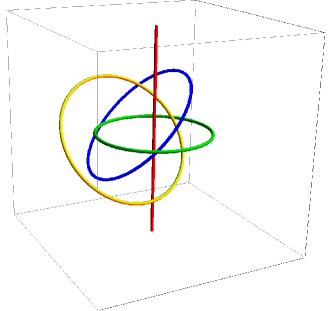
Figure 1: The Hopf map: $f_{H}:\vec{r}\rightarrow\hat{n}$ is shown by displaying contours of equal $\hat{n}$. Points at infinity are all mapped to the same point on the sphere $f_{H}(\infty)=\hat{z}$. In red is $f^{-1}_{H}[\hat{n}=\hat{z}]$, in green $f^{-1}_{H}[-\hat{z}]$, in blue $f^{-1}_{H}[\hat{x}]$, and in yellow $f^{-1}_{H}[\hat{y}]$. Note the unit linking of any pair of curves, which can be used to define the Hopf texture.

Consider a smooth configuration of $\vec{n}(r)$, which can be normalized to give a unit vector $\hat{n}(r)$ at each point. This defines a mapping from each point of three dimensional space, to a unit three vector, which describes the surface of a sphere $S^{2}$. We require that the mapping approaches a constant at infinity: $\hat{n}(|r|\rightarrow\infty)={\rm const}$ (e.g the vacuum). Can all such mappings be smoothly distorted into one another? A surprising result due to Hopf Hopf (1931) 1931, is that there are topologically distinct mappings, which can be labeled by distinct integers $h$ (the Hopf index). No smooth deformation can connect configurations with different Hopf indices. Mathematically, Hopf showed that the homotopy group: $\Pi_{3}[S^{2}]=Z$. A straightforward way to establish the index is to consider the set of points in space that map to a particular orientation of $\hat{n}$. In general this is a curve. If we consider two such orientations, we get a pair of curves. The linking number of the curves is the Hopf index. A configuration with unit Hopf index can be constructed by picking a reference vector $\hat{n}=\hat{z}$, say, and rotating it by the following set of rotations. Any rotation is parameterized by an angle and a direction of rotation. If we take the angle to vary as we move in the radial direction, from $\theta=0$ at the origin, to $\theta=2\pi$ at radial infinity, and take the axis of rotation to be the radial direction $\hat{r}$, this gives a Hopf texture. Using an SU(2) matrix $U(\vec{r})=e^{i\frac{\theta(r)}{2}\hat{r}\cdot\sigma}$ to represent this rotation, the vector field $\hat{n}(\vec{r})=U(\vec{r})\sigma_{z}U^{\dagger}(\vec{r})$ is the unit Hopf texture. This is readily verified by studying which spatial points map to $\hat{n}=\pm\hat{z}$. While the former includes all points at infinity as well as the $z$ axis, the latter is a circle in the $xy$ plane. Clearly these two curves have unit linking number unity (see Figure 1. What is the physical interpretation of this Hopf texture in the context of TIs? A torus of TI (Figure 2) has superconductivity induced on its surface. There is vacuum far away and through the hole of the torus, which counts as a trivial insulator, $\hat{n}=\hat{z}$. The center of the strong topological insulator corresponds to $\hat{n}=-\hat{z}$. On the topological insulator surface $n_{z}=0$, and the superconducting phase varies such that there is a unit vortex trapped in each cycle of the torus. We now argue that such a texture is a fermion.

II Hopf Solitons are Fermions

The ground state of the mean field Hamiltonian (1) for a general texture, has rather low symmetry, and cannot be labeled by spin or U(1) charge quantum numbers. The only quantum number that can be assigned is the parity of the total number of fermions $(-1)^{F}$. Superconducting pairing only changes the number of fermions by an even number, hence one can assign this $Z_{2}$ fermion parity quantum number to any eigenstate. We now argue that the fermion parity of a smooth texture is simply the parity of its Hopf index.

First, we argue that the ground state with a topologically trivial texture has an even number of fermions. As a representative, consider a configuration where the superconductor pairing amplitude is real. This is a time reversal invariant Hamiltonian. If the ground state had an odd number of fermions, it must be doubly degenerate at least, by Kramers theorem. However, the ground state of any smooth texture is fully gapped and hence unique. Thus, this configuration must have an even fermion parity. Now, any other texture in the same topological class can be reached by a continuous deformation, during which the gap stays open. The fermion parity stays fixed during this process. Note, this argument cannot be applied to configurations with nonzero Hopf index, since these necessarily break time reversal symmetry. For example, the configuration shown in Figure 1, contains a pair of vortices.

To find the fermion parity of the nontrivial Hopf configurations, we consider evolving the Hamiltonian between the trivial and $h=1$ configuration. In this process we must have $\vec{n}=0$ at some point, which will allow for the gap to close, and a transfer of fermion parity to potentially occur. Indeed, as shown below in separate calculations, a change in fermion parity is induced when the Hopf index changes by one.

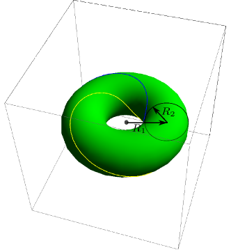
Figure 2: This figure shows a torus of strong topological insulator (green) in vacuum, whose surface is superconducting . There is unit superconductor phase winding about each cycle of the torus. We plot the equal phase contours on the surface whose pairing phase is $0$(blue) and $\pi$(yellow). The unit linking of these curves indicates this is the Hopf mapping.

Figure 3: The spectral flow of the lowest 20 eigenvalues when the pairing on the surface of the topological insulator in Fig. 2 is linearly interpolated between two limits: $\Delta(x,\lambda)=(1-\lambda)\Delta_{0}(x)+\lambda\Delta_{1}(x)$. $\Delta_{0}(x)$ is constant over the whole surface. TOP: $\Delta_{1}(x)$ has a unit phase winding (vortex) in both the $R_{1}$ and $R_{2}$ cycles of the torus, i.e. the Hopf texture. BOTTOM: $\Delta_{1}(x)$ has a unit phase winding in only the $R_{1}$ cycle. It is clear that there is a single level crossing in the TOP case, meaning the ground state fermion parity is changed in the process. The initial state has even fermion parity, so the final state, the Hopf texture,must have odd fermion parity. The calculation is on the cubic lattice model defined in the text, with $R_{1}=13$ and $R_{2}=5$ lattice units, and only points within the torus are retained. Parameters used: $t=M=\lambda=1$, and pairing $|\Delta|=1$.

Numerical Calculation: We study numerically the microscopic topological insulator model defined in reference Hosur et al. (2010), with a pair of orbitals ($\tau_{z}=\pm 1$) on each site of a cubic lattice. The tight binding Hamiltonian $H=\sum_{k}[\psi^{\dagger}_{k}{\mathcal{H}_{k}}\psi_{k}+H_{\rm pair}(k)]$, is written in momentum space using a four component fermion operator $\psi_{k}$ with two orbital and two spin components. Then, ${\mathcal{H}_{k}}=-2t\sum_{a=1}^{3}\alpha_{a}\sin k_{a}-m\beta_{0}[\lambda+\sum_{a=1}^{3}(\cos k_{a}-1)]$, where $(\vec{\alpha},\,\beta_{0})=(\tau_{x}\sigma_{x},\,\tau_{x}\sigma_{y},\,-\tau_{y},\tau_{z})$. For $t,\,m>0$ a strong topological insulator is obtained when $\lambda\in(0,2)$. In addition we introduce onsite singlet pairing $H_{\rm pair}(k)=\Delta[\psi^{\dagger}_{k}]^{\rm T}\sigma_{y}\psi^{\dagger}_{-k}+\,{\rm h.c.}$. Note, when $\lambda\approx 0,\,\vec{k}\approx(0,\,0,\,0)$, Eqn. 1 is recovered as the low energy theory.

The energy spectrum is studied as we interpolate between a topologically trivial texture ($h=0$) and the Hopf texture ($h=1$). We choose to define a torus shaped strong topological insulator with trivial insulator (vacuum) on the outside, as in figure 2. The surface is gapped by superconducting pairing $\Delta$, which in the trivial texture is taken to be real $\Delta_{0}$. In the Hopf texture, the superconducting pairing $\Delta_{1}$ has a phase that winds around the surface, with a unit winding about both cycles of the torus. This can be interpreted as ’vortices’ inside the holes of the torus. Note, the vortex cores are deep inside the insulators, so there is a finite gap in the Hopf texture. We interpolate between these two fully gapped phases be defining $\Delta(\lambda)=\lambda\Delta_{1}+(1-\lambda)\Delta_{0}$ and changing $\lambda=0\rightarrow 1$. On the way, the gap must close since the two textures differ in topology. We study the evolution of eigenvalues as shown in figure 3. We find that exactly one pair of $\pm E$ eigenvalues are pumped through zero energy. As argued below, this signals a change in the fermion parity of the ground state on the two sides. Since the trivial texture has even fermion parity from time reversal symmetry, the Hopf texture must carry odd fermion number. No such odd level crossings occur for topologically trivial textures (eg. phase winding through only one cycle of the torus).

To see why the crossing of a $\pm E$ conjugate pair of levels corresponds to a change in fermion number, consider a single site model $H=E_{0}(c^{\dagger}c-cc^{\dagger})$. This has a pair of single particle levels at $\pm E_{0}$, which will cross if we tune $E_{0}$ from say positive to negative values. However, writing this Hamiltonian in terms of the number operators $H=E_{0}(2\hat{n}-1)$, shows that the ground state fermion number changes from $n=0$ to $n=1$ in this process. Thus the ground state fermion parity is changed whenever a pair of conjugate levels cross zero energy.

The Pfaffian: Previously, the ground state fermion parity was found by interpolating between two topological sectors. Can one directly calculate the fermion parity for a given Hamiltonian’s ground state? We show this is achieved by calculating the Pfaffian of the Hamiltonian in the Majorana basis. The Pfaffian of an antisymmetric matrix is the square root of the determinant - but with a fixed sign. It is convenient to recast the Hamiltonian in terms of Majorana or real fermions defined via $\psi_{a}=(\chi_{1a}+i\chi_{2a})/2$. Since a pair of Majorana fermions anticommute $\{\chi_{i},\,\chi_{j}\}=\delta_{ij}$, the Hamiltonian written in these variables will take the form:

$$H=-i\sum_{ij}{\rm\bf h}_{ij}\chi_{i}\chi_{j}$$ (2)

where ${\rm\bf h}_{ij}$ is an even dimensional antisymmetric matrix, with real entries and the Majorana fields appear as a vector $\chi=(\dots,\,\chi_{1a},\chi_{2a},\,\dots)$, where $a$ refers to site, orbital and spin indices. The $\pm E$ symmetry of the spectrum is an obvious consequence of $h$ being an antisymmetric matrix. The ground state fermion parity in this basis is determined via:

$$(-1)^{F}=sign\left[{\rm Pfaffian}({\rm\bf h})\right]$$ (3)

We numerically calculated the Pfaffian of a Hamiltonian with a single Hopf texture for small systems and confirmed it has a negative sign. In contrast, the trivial Hopf texture Hamiltonian has positive Pfaffian in the same basis.

Finally, we mention that it is possible to confirm the numerical results analytically, by solving for the low energy modes in the vicinity of the vortex core, where the insulating mass term is set to be near zero. The linking of vortices in the Hopf texture plays a crucial role in deriving this result. In the Appendix, we discuss how this result is connected to the three dimensional non-Abelions in the hedgehog cores of Ref Teo and Kane, 2010.

A Two Dimensional Analog: We briefly mention a two dimensional analog of the physics described earlier. Note, eqn. 1 with the third component of momentum absent $p_{z}=0$, describes a quantum spin Hall insulator (trivial insulator) when $m>0$ ($m<0$), in the presence of singlet pairing $\Delta$. Again, as before a three vector characterizes a fully gapped state, and the nontrivial textures are called skyrmions ($\Pi_{2}(S_{2})=Z$). A unit skyrmion can be realized with a disc of quantum spin Hall insulator with superconductivity on the edge, whose phase winds by $2\pi$ on circling the disc. Again, one can show that the skyrmion charge $Q$ determines the fermion parity $(-1)^{Q}=(-1)^{F}$. An important distinction from the three dimensional case is that the low energy theory here has a conserved charge. If instead of superconductivity, one gapped out the edge states with a time reversal symmetry breaking perturbation which had a winding, then this charge is the electrical charge. It is readily shown that the charge is locked to the skyrmion charge $Q$. Hence odd strength skyrmions are fermions. This is closely analogous to the Quantum Hall ferromagnet, where charged skyrmions also occur Lee and Kane (1990); Sondhi et al. (1993). Returning to the case with pairing, since that occurs on a one dimensional edge, it is difficult to draw a clear-cut separation between fermions and collective bosonic coordinates, in contrast to the higher dimensional version. Hence we focus on the 3DTIs.

III Effective Theory and Topological Term

The gap to the $\psi$ fermions never vanishes since $|\vec{n}|>0$, so one can integrate out the fermions to obtain a low energy theory written solely in terms of the bosonic order parameter $\vec{n}$. How can this field theory describe a fermionic texture? As described below, this is accomplished by a topological Berry phase term which appears in the effective action for the $\hat{n}$ field.

In computing the topological term, it is sufficient to consider a gap whose magnitude is constant $\vec{n}(r,t)=M\hat{n}(r,t)$. Integrating out the fermion fields with action $S_{f}=\int d^{4}\;x[\psi^{\dagger}\partial_{t}\psi-H_{f}]$, (the integral is over space and (Euclidean) time), one obtains the effective action for the bosonic fields:

$$e^{-S_{B}(\hat{n}(r,t)}=\int{\mathcal{D}}\psi{\mathcal{D}}\psi^{\dagger}e^{-S_{f}[\hat{n},\psi,\psi^{\dagger}]}$$ (4)

This computation may be performed using a gradient expansion, i.e. assuming slow variation of the $\hat{n}$ field over a scale set by the gap. Two terms are obtained: $S_{b}=S_{0}+S_{\rm top}$. The first is a regular term that penalizes spatial variation: $S_{0}=\frac{1}{2g}\int(\partial_{\mu}\hat{n})^{2}$. The second is a topological term which assigns a different amplitude to topologically distinct spacetime configurations of $\hat{n}$. Assuming $\hat{n}(\infty)=const$, these configurations are characterized by a $Z_{2}$ distinction ($\Pi_{4}(S_{2})=Z_{2}$)Nakahara (2003). That is, there are two classes of maps - the trivial map, which essentially corresponds to the uniform configuration, and a non-trivial class of maps, which can all be smoothly related to a single representative configuration $\hat{n}_{1}(r,t)$. If the function $\Gamma[\{\hat{n}(r,t)\}]=0,\,1$ measures the topological class of a spacetime configuration, then the general form of the topological term is $S_{\rm top}=i\theta\Gamma[\{\hat{n}(r,t)\}]$. The topological angle $\theta$ can be argued to take on only two possible values $0,\,\pi$, since composing a pair of nontrivial maps, leads to the trivial map. Via an explicit calculation, outlined below, we find $\theta=\pi$. Let us first examine the consequences of such a term. The nontrivial texture $\hat{n}_{1}(r,t)$ can be described as a Hopfion-antiHopfion pair being created at time $t_{1}$, the Hopfion being rotated slowly by $2\pi$, and then being combined back with the anitHopfion at a later time $t_{2}$ Wilczek and Zee (1983). The topological term assigns a phase of $e^{i\pi}$ to this configuration. This is equivalent to saying the Hopfion is a fermion, since it changes sign on $2\pi$ rotation.

Calculating the topological term requires connecting the pair of topologically distinct configurations. To do this in a smooth way keeping the gap open at all times requires enlarging the order parameter space for this purpose. If ${\bf m}(r,t,\lambda)$ is an element of this enlarged state that smoothly interpolates between the trivial configuration ${\bf m}(r,t,0)={\rm const.}$ and the nontrivial one ${\bf m}(r,t,1)=\hat{n}_{1}(r,t)$, as we vary $\lambda$, then one can analytically calculate the change in the topological term $\partial S_{\rm top}/\partial\lambda$, and integrate it to get the required result Elitzur and Nair (1984); Klinkhamer (1991); Abanov (2000); Abanov and Wiegmann (2000). The key technical point is finding a suitable enlargement of our order parameter space $S_{2}$. Remembering that this can be considered as $S_{2}=SU(2)/SO(2)$, we can make a natural generalization $M_{3}=SU(3)/SO(3)$. The latter has all the desirable properties of an expanded space, eg. there are no nontrivial spacetime configurations, so everything can be smoothly connected ($\Pi_{4}(M_{3})=0$). This extension allows us to calculate the topological term, (as explained in detail in the methods section), which yields $\theta=\pi$.

IV Physical Consequences

We now discuss two kinds of physical consequences arising from fermionic Hopfions. The first relies on the dynamical nature of the superconducting order parameter, while the second utilizes the Josephson effect to isolate an anomalous response. The first class conceptually parallels experiments used to identify skyrmions in quantum hall ferromagnets. There, when skyrmions are the cheapest charge excitations, they are detected on adding electrons to the system Barrett et al. (1995).

Consider surface superconductivity on a mesoscopic torus shaped topological insulator as in Figure 2. The Hopf texture corresponds to unit phase winding in each cycle of the torus. The energy cost, $E_{H}=(\rho_{s}/2)\int(\nabla\phi)^{2}d^{2}x$ is simply proportional to the superfluid density $E_{H}=A\rho_{s}$, where $A$ is in general an $O(1)$ constant. If we have $E_{H}<\Delta$ the superconducting gap, then the Hopfion is the lowest energy fermionic excitation. Tunneling a single electron onto the surface should then spontaneously generate these phase windings in equilibrium. Measuring the corresponding currents (eg. via an RF squid) can be used to establish the presence of the Hopf texture. A daunting aspect of this scheme is to obtain a fully gapped superconductor with $\rho_{s}<\Delta$.

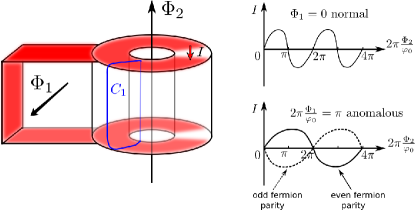
Figure 4: Anomalous Josephson Response connected to fermionic Hopfions: An annular cylinder of TI with pairing induced on the top and bottom surfaces via proximity to a superconductor (present in the red regions) is shown. Tuning the flux to $\Phi_{1}\approx\varphi_{0}/2$, induces a vortex in the $C_{1}$ cycle. Now, the Josephson effect on tuning $\Phi_{2}$ will be anomalous, with a part that is not periodic in the flux $\varphi_{0}$. This is directly related to the change in ground state fermion parity at $\Phi_{2}=2\pi(\varphi_{0}/2\pi)$, where the Hopf texture is realized. Adding a fermion inverts this current, indicating that the ground state in this sector is at $\Phi_{2}=2\pi(\varphi_{0}/2\pi)$. If however $\Phi_{1}\approx 0$, there is no vortivity in the $C_{1}$ cycle, and the Josephson effect is the usual one, periodic in the flux quantum $\varphi_{0}=h/2e$.

A different approach relies on the Josephson effect as illustrated in Figure 4. A hollow cylinder of topological insulators is partially coated with superconductor on the top and bottom surfaces, forming a pair of Josephson junctions. A unit vortex along the $C_{1}$ cycle can be induced by enforcing a phase difference of $\pi$ between the top and bottom surfaces, using the flux $\Phi_{1}={\mathcal{\varphi}}_{0}/2$ (where $\varphi_{0}=h/2e$ is the superconductor flux quantum). Now, the vorticity enclosed by the annulus determines the Hopf number, and hence the ground state fermion parity. This vorticity can be traded for magnetic flux $\Phi_{2}$ (parameterized via $f_{2}=2\pi(\Phi_{2}/\varphi_{0})$) threading the cylinder, since only $\nabla\phi-eA$ is gauge invariant. Consider beginning in the ground state with $f_{2}=0$ and then tuning to $f_{2}=2\pi$. One is now in an excited state since the ground state at this point has odd fermion parity. This must be reflected in the Josephson current $I$. We argue this implies doubling the flux period of the Josephson current. Since $I=\partial E(\Phi_{2})/\partial\Phi_{2}$, the area under the $(I,\,\Phi_{2})$ curve :$\int_{0}^{\varphi_{0}}d\Phi_{2}\,I[\Phi_{2}]=E[\varphi_{0}]-E[0]>0$ is the excitation energy which does not vanish. Hence, the Josephson current is not periodic in flux $\varphi_{0}$, as in usual Josephson junctions. If we started with an odd fermion number to begin with, then the state of affairs would be reversed - the ground state would be achieved at multiples of $f_{2}=2\pi$. The ground state with a particular fermion parity can be located by studying the slope of the current vs phase curve. Since the energy of the ground state increases on making a phase twist $\partial I/\partial\Phi_{2}=\partial^{2}E/\partial\Phi_{2}^{2}>0$, it is associated with a positive $I\,{\rm vs}\,\Phi_{2}$ slope. This positive slope will be at even (odd) multiples of $f_{2}=2\pi$ for even (odd) fermion parity. If on the other hand unit vorticity was not induced in the cycle $C_{1}$, (eg. if $\Phi_{1}\sim 0$), the Josephson relation would be the usual one - i.e. one that is periodic in $f_{2}=2\pi$. This is summarized in Figure 4.

Note, a similar anomalous $4\pi$ Josephson periodicity was pointed out in the context pf the 2D QSH case with proximate superconductivity in Fu and Kane (2009). We interpret this result in terms of the fermionic nature of the solitons there - which lends a unified perspective. In the 3D case, the Hopf texture allows one to tune between the normal and anomalous Josephson effect by tuning the $C_{1}$ vorticity via $\Phi_{1}$.

V Conclusions

The low energy field theory of the superconductor-TI system was derived and shown to possess a topological Berry phase term, which leads to fermionic Hopf solitons. We note that topological terms are particularly important in the presence of strong quantum fluctuations. For example, in one dimension where fluctuations dominate, the Berry phase term of the spin 1/2 Heisenberg chainHaldane (1988) leads to an algebraic phase. By analogy, it would be very interesting to study the destruction of superconductivity on a TI surface driven by quantum fluctuations. The Berry phase, or relatedly, the fact that a conventional insulator must break time reversal on the TI surface, will provide an interesting twist to the well know superconductor-insulator transition studied on conventional substrates Haviland et al. (1989).

We acknowledge helpful discussions with C. Kane, A. Turner and S. Ryu. A.V. and P.H. were supported by NSF DMR- 0645691.

VI Appendix

A. Connections to 3D non-Abelian statistics

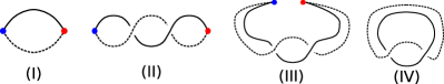
Figure 5: (color online) Creating a Hopf soliton by a hedgehog-antihedgehog pair. The blue(red) dot is the hedgehog(antihedgehog). The solid and dotted lines are preimages of two different points on the 2-sphere. (I) creating a pair of hedge and antihedgehog - these could be a vortex-antivortex pair on the surface of a topological insulator (II) rotating the hedgehog by $2\pi$ while leaving the antihedgehog invariant (III)(IV) annihilating the hedgehog-antihedgehog pair. The final state in (IV) clearly shows linking number $1$ of the two preimage loops, which indicates the non-trivial Hopf index.

It is well known that vortices piercing a superconductor on the topological insulator surface carry Majorana zero modes in their cores Fu and Kane (2008); Teo and Kane (2010). In the $\vec{n}$ vector representation of Eq. (1), this corresponds to a hedgehog defectTeo and Kane (2010), a singular configuration where the vector points radially outwards from the center. Although in this paper we only work with smooth textures, we discuss below an indirect connection with those works. Note, we can go from a trivial texture to the Hopf texture by creating a hedgehog-antihedgehog pair, rotating one of them by an angle of $2\pi$, and annihilating them to recover a smooth texture. This is just the Hopf texture, as can be seen in the Figure 5. However, as pointed out in Ref. Teo and Kane (2010), in the process of rotation, the Majorana mode changes sign. This signals a change in fermion parity, consistent with our results.

B. Calculation of Berry’s phase. We begin with:

$$H =\mathbf{\Psi}^{\dagger}v_{F}(-i\partial_{i}\alpha_{i})\mathbf{\Psi}+M\mathbf{\Psi}^{\dagger}(n_{1}\beta_{0}+n_{2}\beta_{5}\eta_{x}+n_{3}\beta_{5}\eta_{z})\mathbf{\Psi},$$ (5)

where, $\mathbf{\Psi}$ is the fermion in majorana basis (8-component), $n_{1}$ is the insulator mass and $n_{2},n_{3}$ are the superconductivity masses, and the standard five anticommuting 4 by 4 Dirac matrices in the Majorana basis (where the $\alpha$s are symmetric and $\beta$s are antisymmetric matrices):

$$\alpha_{1}=\sigma_{z},\;\alpha_{2}=\tau_{x}\sigma_{x},\;\alpha_{3}=-\tau_{z}\sigma_{x},\;\beta_{0}=\tau_{y}\sigma_{x},\;\beta_{5}=\sigma_{y}.$$ (6)

We further assume the order parameters $n_{i}$ are restricted to unit 2-sphere: $\sum_{i}n_{i}^{2}=1$ so that $\hat{n}=(n_{1},n_{2},n_{3})$ is a unit vector living on $S^{2}$.

We need to show that starting from this fermionic model Eq.(5) and integrating out the fermions, the obtained $S^{2}$-NLSM has an imaginary term (topological Berry’s phase) $i\theta H_{\pi_{4}(S^{2})}(\hat{n}(x,y,z,t))$ with $\theta=\pi$ in the action (from now on we use $H_{\pi_{n}(M)}$ to denote the homotopy index of a mapping.). Because this term is non-perturbative, in order to compute it, we need to embed the manifold $S^{2}$ into a larger manifold $M$ with $\pi_{4}(M)=0$, which allows us to smoothly deform a $H_{\pi_{4}(S^{2})}(\hat{n}(x,y,z,t))=1$ mapping to a constant mapping. This means that a $H_{\pi_{4}(S^{2})}(\hat{n}(x,y,z,t))=1$ mapping can be smoothly extended over the 5-dimension disk: $V(x,y,z,t,\rho):D^{5}\rightarrow M$ ($\rho\in[0,1]$) such that on the boundary: $V(x,y,z,t,\rho=1)=\hat{n}(x,y,z,t)$ and $V(x,y,z,t,\rho=0)=V_{0}$ is constant. With an extension $V$, we can perturbatively keep track of the total change of Berry’s phase when going from a constant mapping to a non-trivial mapping.

How to find a suitable $M$? We note the global symmetry of model Eq.(5) in the massless limit is $U(1)_{chiral}\times SU(2)_{isospin}$, whose generators are:

$$U(1)_{chiral}: \;\gamma_{5}=-i\beta_{0}\beta_{5} SU(2)_{isospin}: \;\eta_{y},\gamma_{5}\{\eta_{x},\eta_{z}\}.$$ (7)

In our convention, $\beta_{0},\beta_{5},\gamma_{5}$ are all anti-symmetric matrices. Starting from a given mass, for instance, $\mathbf{\Psi}^{\dagger}\beta_{0}\mathbf{\Psi}$, one can generate the full order parameter manifold by action of $SU(2)_{isospin}$: $\mathbf{\Psi}^{\dagger}W\beta_{0}W^{\dagger}\mathbf{\Psi}$. $SU(2)_{isospin}$ is broken down to $U(1)$, the invariant group generated by $\eta_{y}$. Thus the order parameter space is $SU(2)/U(1)=S^{2}$.

Now we generalize the 8-component majorana fermion $\mathbf{\Psi}$ to 12-component $\mathbf{\tilde{\Psi}}$. The 2-dimensional $\eta_{x,y,z}$-space is enlarged to a 3-dimensional space, and we let the eight $\lambda_{i}$-matrices ($i=1,2...8$) of the standard $SU(3)$ generators(see, e.g., page 61 in Georgi (1982)) act within this 3-dimensional space, among which $\lambda_{2},\lambda_{5},\lambda_{7}$ are antisymmetric while others are symmetric. And $\lambda_{1,2,3}$ are just the old $\eta_{x,y,z}$ matrices. The symmetry of the generalized massless theory of $\mathbf{\tilde{\Psi}}$: $H=\mathbf{\tilde{\Psi}}^{\dagger}(-i\partial_{i}\alpha_{i})\mathbf{\tilde{\Psi}}$ is $U(1)_{chiral}\times SU(3)_{isospin}$, where the generators of the $SU(3)_{isospin}$ are $\lambda_{2},\lambda_{5},\lambda_{7}$,$\gamma_{5}\{\lambda_{1},\lambda_{3},\lambda_{4},\lambda_{6},\lambda_{8}\}$.

Starting from a given mass $\mathbf{\tilde{\Psi}}^{\dagger}\beta_{0}\mathbf{\tilde{\Psi}}$, we use $SU(3)_{isospin}$ to generate the order parameter manifold: $\mathbf{\tilde{\Psi}}^{\dagger}U\beta_{0}U^{\dagger}\mathbf{\tilde{\Psi}}\equiv\mathbf{\tilde{\Psi}}^{\dagger}V\mathbf{\tilde{\Psi}}$, $U\in SU(3)_{isospin}$. It is clear that the $SO(3)$ subgroup generated by $\lambda_{2},\lambda_{5},\lambda_{7}$ is the invariant group and the order parameter manifold is $M_{3}\equiv SU(3)/SO(3)$. We thus embed the original order parameter manifold $S^{2}$ into $M_{3}$, and it is known that $\pi_{4}(M_{3})=0$(Auzzi and Shifman (2007)).

The idea is to smoothly extend a $H_{\pi_{4}(S^{2}))}=1$ mapping over $D^{5}$ (denote by $V(x,y,z,t,\rho)$) by embedding $S^{2}$ into $M_{3}$. In fact if we can extend a $H_{\pi_{4}(SU(2))}=1$ mapping over $D^{5}$ (denote by $U(x,y,z,t,\rho)$) by embedding $SU(2)_{isospin}$ into $SU(3)_{isospin}$, it will generate the extension $V$ by $V=U\beta_{0}U^{\dagger}$. This is because a $H_{\pi_{4}(S^{2}))}=1$ mapping can be thought as a combination of a $H_{\pi_{4}(SU(2))}=1$ mapping and a Hopf $H_{\pi_{3}(S^{2})}=1$ mapping. Such an extension $U:D^{5}\rightarrow SU(3)_{isospin}$ has already been explicitly given by Witten (see Eq.(9-13) in RefWitten (1983)), which we will term it Witten’s map. Witten’s map was introduced to compute a $i\theta H_{\pi_{4}(SU(2))}$ topological Berry’s phase. Basically, on the boundary $\partial D^{5}=S^{4}$ ($\rho=1$), Witten’s map is a $H_{\pi_{4}(SU(2))}=1$ mapping defined as a rotating $H_{\pi_{3}(SU(2))}=1$ soliton (by $2\pi$) along the time direction. This $H_{\pi_{4}(SU(2))}=1$ mapping at $\rho=1$ is smoothly deformed into a trivial mapping at $\rho=0$ by embedding $SU(2)$ into $SU(3)$.

We use Witten’s map to generate $V$, with which we compute the Berry’s phase perturbatively by a large mass expansionAbanov and Wiegmann (2000); Hosur et al. (2010) of Lagrangian:

$$L=\mathbf{\tilde{\Psi}}^{\dagger}[\partial_{\tau}+i\partial_{i}\alpha_{i}]\mathbf{\tilde{\Psi}}+M\mathbf{\tilde{\Psi}}^{\dagger}V\mathbf{\tilde{\Psi}}\equiv\mathbf{\tilde{\Psi}}^{\dagger}[D]\mathbf{\tilde{\Psi}},$$ (8)

where $D=[\partial_{\tau}+i\partial_{i}\alpha_{i}+MV]$ and partition function is $Z=\int\mathcal{D}\mathbf{\tilde{\Psi}}^{\dagger}\mathcal{D}\mathbf{\tilde{\Psi}}\mathcal{D}Ve^{-\int d^{4}xL}$. After integrating out fermion, we obtain a NLSM of $V$: $\tilde{L}=-\frac{1}{2}\mbox{Tr}\ln[\partial_{\tau}+i\partial_{i}\alpha_{i}+MV]$. Here the factor $1/2$ is because we are integrating out majorana fields. If there is a variation $\delta V$, the variation of the imaginary part $\Gamma\equiv\mbox{Im}(\tilde{L})$ is:

$$\delta\Gamma=\frac{-K}{2}\int dx^{4}\epsilon^{\alpha\beta\gamma\mu}\mbox{Tr}\{\gamma_{5}V\partial_{\alpha}V\partial_{\beta}V\partial_{\gamma}V\partial_{\mu}V\delta V\}$$ (9)

where $K=\int\frac{d^{4}p}{(2\pi)^{4}}\frac{M^{6}}{(p^{2}+M^{2})^{5}}=\frac{1}{192\pi^{2}}$. Denoting $\partial_{\rho}=\partial_{4}$, after some algebra, the Berry’s phase can be written in the fully antisymmetric way:

$$\Gamma=\frac{-K}{10}\int dx^{5}\epsilon^{\alpha\beta\gamma\mu\nu}\mbox{Tr}\{\gamma_{5}V\partial_{\alpha}V\partial_{\beta}V\partial_{\gamma}V\partial_{\mu}V\partial_{\nu}V\}$$ (10)

In fact $\Gamma$ is not fully well defined because the ambiguity of the extension of $\hat{n}(x,y,z,t)$ to the 5-disk: two different extensions $V(x,y,z,t,\rho)$ can differ by a mapping $S^{5}\rightarrow M_{3}$. We will soon show that this ambiguity means that $\Gamma$ is well defined up to $\mbox{mod }2\pi$.

As $V$ is generated by $U$, plugging $V=U\beta_{0}U^{\dagger},U\in SU(3)_{isospin}$ in Eq.(10), one can further simplify it by trace out the $\beta_{0,5}$ space. Firstly note that $\partial_{\mu}V=U[U^{\dagger}\partial_{\mu}U,\beta_{0}]U^{\dagger}$, and because $U^{\dagger}\partial_{\mu}U$ is an element of the $SU(3)_{isospin}$ Lie algebra spanned by $\lambda_{2},\lambda_{5},\lambda_{7}$,$\gamma_{5}\{\lambda_{1},\lambda_{3},\lambda_{4},\lambda_{6},\lambda_{8}\}$, $[U^{\dagger}\partial_{\mu}U,\beta_{0}]$ simply picks out the latter five generators. After some algebra, one finds

$$\Gamma= \frac{1}{15\pi^{2}}\int dx^{5}\epsilon^{\alpha\beta\gamma\mu\nu}\mbox{Tr}(g^{-1}\partial_{\alpha}g)_{\perp}(g^{-1}\partial_{\beta}g)_{\perp}(g^{-1}\partial_{\gamma}g)_{\perp}(g^{-1}\partial_{\mu}g)_{\perp}(g^{-1}\partial_{\nu}g)_{\perp}\},$$ (11)

where $g$ is defined as the corresponding 3 by 3 $SU(3)$ matrix of $U$: if $U$ is the exponential of $a_{1}\lambda_{2}+a_{2}\lambda_{5}+a_{3}\lambda_{7}+a_{4}\gamma_{5}\lambda_{1}+a_{5}\gamma_{5}\lambda_{3}+a_{6}\gamma_{5}\lambda_{4}+a_{7}\gamma_{5}\lambda_{6}+a_{8}\gamma_{5}\lambda_{8}$, then $g$ is the exponential of $a_{1}\lambda_{2}+a_{2}\lambda_{5}+a_{3}\lambda_{7}+a_{4}\lambda_{1}+a_{5}\lambda_{3}+a_{6}\lambda_{4}+a_{7}\lambda_{6}+a_{8}\lambda_{8}$. $g$ is nothing but the Witten’s map. And $(g^{-1}\partial_{\mu}g)_{\perp}$ denotes the symmetric part: $(g^{-1}\partial_{\mu}g)_{\perp}=\big{[}(g^{-1}\partial_{\mu}g)+(g^{-1}\partial_{\mu}g)^{T}\big{]}/2$.

We simply need to compute $\Gamma$ by integration. Because it is clear that $\Gamma$ can only be $0$ or $\pi$ (mod $2\pi$), a numerical integration is enough to determine it unambiguously. We performed integration Eq.(11) with Witten’s map $g$ by standard Monte Carlo approach, and find $\Gamma=(1.000\pm 0.005)\pi$. This proves that Hopf-skyrmion is a fermion. In addition it confirms that $\Gamma$ is well-defined only up to mod $2\pi$: different extensions of $g$ can differ by a doubled Witten’s map is known to have $H_{\pi_{5}(SU(3))}=1$, and the above calculation indicate that this ambiguity only add an integer times $2\pi$ in $\Gamma$.

References

- Hasan and Kane (2010) M. Z. Hasan and C. L. Kane, arXiv:1002.3895v1 (2010).
- Qi and Zhang (2010) X.-L. Qi and S.-C. Zhang, Physics Today 63, 33 (2010).
- Essin et al. (2009) A. M. Essin, J. E. Moore, and D. Vanderbilt, Phys. Rev. Lett. 102, 146805 (2009).
- Yu et al. (2010) R. Yu, W. Zhang, H. J. Zhang, S. C. Zhang, X. Dai, and Z. Fang, arXiv:1002.0946 (2010).
- Ran et al. (2009) Y. Ran, Y. Zhang, and A. Vishwanath, Nat Phys 5, 298 (2009).
- Fu and Kane (2008) L. Fu and C. L. Kane, Phys. Rev. Lett. 100, 096407 (2008).
- Jackiw and Rossi (1981) R. Jackiw and P. Rossi, Nuclear Physics B 190, 681 (1981).
- Read and Green (2000) N. Read and D. Green, Phys. Rev. B 61, 10267 (2000).
- Ivanov (2001) D. A. Ivanov, Phys. Rev. Lett. 86, 268 (2001).
- Hor et al. (2010) Y. S. Hor, A. J. Williams, J. G. Checkelsky, P. Roushan, J. Seo, Q. Xu, H. W. Zandbergen, A. Yazdani, N. P. Ong, and R. J. Cava, Phys. Rev. Lett. 104, 057001 (2010).
- Giamarchi (2003) T. Giamarchi, Quantum Physics in One Dimension (Oxford University Press, 2003).
- Sondhi et al. (1993) S. L. Sondhi, A. Karlhede, S. A. Kivelson, and E. H. Rezayi, Phys. Rev. B 47, 16419 (1993).
- Lee and Kane (1990) D.-H. Lee and C. L. Kane, Phys. Rev. Lett. 64, 1313 (1990).
- Barrett et al. (1995) S. E. Barrett, G. Dabbagh, L. N. Pfeiffer, K. W. West, and R. Tycko, Phys. Rev. Lett. 74, 5112 (1995).
- Teo and Kane (2010) J. C. Y. Teo and C. L. Kane, Phys. Rev. Lett. 104, 046401 (2010).
- Hopf (1931) H. Hopf, Mathematische Annalen 104, 637 (1931).
- Hosur et al. (2010) P. Hosur, S. Ryu, and A. Vishwanath, Phys. Rev. B 81, 045120 (2010).
- Nakahara (2003) M. Nakahara, Geometry, Topology and Physics (Inst of Physics Pub Inc, 2003).
- Wilczek and Zee (1983) F. Wilczek and A. Zee, Phys. Rev. Lett. 51, 2250 (1983).
- Elitzur and Nair (1984) S. Elitzur and V. P. Nair, Nuclear Physics B 243, 205 (1984).
- Klinkhamer (1991) F. R. Klinkhamer, Physics Letters B 256, 41 (1991).
- Abanov (2000) A. G. Abanov, Physics Letters B 492, 321 (2000).
- Abanov and Wiegmann (2000) A. G. Abanov and P. B. Wiegmann, Nuclear Physics B 570, 685 (2000).
- Fu and Kane (2009) L. Fu and C. L. Kane, Phys. Rev. B 79, 161408 (2009).
- Haldane (1988) F. D. M. Haldane, Phys. Rev. Lett. 61, 1029 (1988).
- Haviland et al. (1989) D. B. Haviland, Y. Liu, and A. M. Goldman, Phys. Rev. Lett. 62, 2180 (1989).
- Georgi (1982) H. Georgi, Lie Algegras in Particle Physics (Addson-Wesley Publishing Company, Inc., 1982).
- Auzzi and Shifman (2007) R. Auzzi and M. Shifman, Journal of Physics A: Mathematical and Theoretical 40, 6221 (2007).
- Witten (1983) E. Witten, Nuclear Physics B 223, 433 (1983).