Magnetic properties of a strongly correlated system on the Bethe lattice

Abstract

We study the influence of an external magnetic field $h$ on the phase diagram of a system of Fermi particles living on the sites of a Bethe lattice with coordination number $z$ and interacting through on-site $U$ and nearest-neighbor $V$ interactions. This is a physical realization of the extended Hubbard model in the narrow-band limit. Our results establish that the magnetic field may dramatically affect the critical temperature below which a long-range charge ordered phase is observed, as well as the behavior of physical quantities, inducing, for instance, magnetization plateaus in the magnetization curves. Relevant thermodynamic quantities - such as the specific heat and the susceptibility - are also investigated at finite temperature by varying the on-site potential, the particle density and the magnetic field.

Statistical models on the Bethe lattice are of considerable interest since they admit a direct analytical approach for a number of problems that may be otherwise intractable on Euclidean lattices. Due to the peculiar structure of the lattice, several interesting physical problems involving interactions are exactly solvable when defined on the Bethe lattice baxter . There is a general interest in the study of models defined on such lattices which goes beyond physics. Being a dendrimer of infinite generation, the Bethe lattice is attractive both for basic and applied interdisciplinary research involving chemistry, physics, biology, pharmaceutics, and medicine dendri .

In a recent paper, we provided a comprehensive and systematic analysis of the extended Hubbard model in the narrow-band (atomic) limit (AL-EHM) on the Bethe lattice with arbitrary coordination number $z$ mancinis09 . Within the Green’s function and equations of motion formalism, we exactly solved the model and, by considering relevant physical quantities in the whole space of the model parameters, we investigated the finite temperature phase diagram, for both attractive and repulsive on-site and intersite interactions. The aim of the present paper is twofold. First, we would like to further develop our previous work, by extending it to a more general situation in which a finite magnetization may be induced by an external magnetic field. Secondly, the AL-EHM on the Bethe lattice exhibits interesting features at low temperatures such as the existence of magnetic plateaus. Here, we address the problem of determining the effect on the phase diagram and on the behavior of several thermodynamic quantities of the presence of a uniform magnetic field, introduced through a Zeeman term. We study the properties of the system as functions of the external parameters $n$, $T/V$, $U/V$ and $h/V$, allowing for the on-site interaction $U$ to be both repulsive and attractive. In fact, the parameter $U$ can represent the effective interaction coupling taking into account also other interactions. Throughout the paper, we consider a repulsive intersite interaction $V$ and we set $V=1$ as the unit of energy, taking the Boltzmann’s constant $k_{B}=1$. In the absence of a magnetic field, the phase diagram in the plane ($n,T$) exhibits a transition line along the temperature axis, below which translational invariance is broken mancinis09 . The Bethe lattice effectively splits in two sublattices with different thermodynamic properties. As a result, a charge ordered (CO) phase, characterized by a different distribution of the electrons in alternating shells, is established for pertinent values of the particle density. A finite magnetic field can have dramatic effect on the phase diagram: for instance, when $U<0$, the reentrant behavior observed for $h=0$ mancinis09 disappears and one finds, above a certain value of $h$, a CO phase for $n>1/z$. This should be compared with the case $h=0$, where the CO phase is observed only for $n>2/z$ when $U<0$ mancinis09 . The characteristic lobe structure, exhibited by the critical temperature as a function of the particle density, shrinks by augmenting the magnetic field. By further increasing $h$, the CO phase is suppressed in the particle density range $0.75<n<0.85$ and $1.15<n<1.25$ at $h=h_{T}=zV/2-U/2$; the lobe splits in three separated lobes centered around $n=0.5$, 1, and $1.5$, respectively. The central lobe eventually vanishes by increasing $h$. A similar behavior is observed also for $U>0$.

The magnetic properties of the system depend on the value of the particle density and of the on-site potential. At low temperatures, and for attractive on-site interactions, the magnetic field does not play any role if its intensity is $h<|U|/2$: the ground state is a collection of shells with doubly occupied sites (doublons) surrounded by empty shells. The magnetic energy is not strong enough to break the doublons. On the other hand, for strong repulsive on-site interactions, it is sufficient a small nonzero value of the magnetic field to have a finite magnetization. In the intermediate region, the competition among $U$, $V$ and $h$ determines the phase structure. For all values of the particle density, one finds a critical value of the magnetic field $h_{s}$ - dramatically depending on $U$ and $n$ - above which the ground state is paramagnetic. In this state, every occupied site contains one and only one electron, aligned along the direction of $h$. For strong repulsive on-site interactions, $h_{s}=0$, i.e., the spin are polarized as soon as the magnetic field is turned on. Furthermore, for attractive on-site interactions and $0.5<n\leq 1$, one observes the existence of two critical fields, namely: $h_{c}$, up to which no magnetization is observed, and $h_{s}$, marking the beginning of full polarization. This is analogous to the finite field behavior of the $S=1$ Haldane chain haldane .

The addition of a homogeneous magnetic field does not dramatically modify the framework of calculation given in Ref. mancinis09 , provided one takes into account the breakdown of the spin rotational invariance. For the sake of comprehensiveness, in the next section, we briefly report the analysis leading to the exact solution of the AL-EHM on the Bethe lattice in the presence of a magnetic field. Then, we investigate the phase diagram in the space $n$, $T/V$, $U/V$ by varying $h$ and we observe that, above a critical value of $h$, the CO region shrinks due to the presence of a finite magnetic field. We also analyze the magnetic properties of the system and find magnetic plateaus in the magnetization curve. Finally, last section is devoted to our conclusions.

I Exactly solvable model

When defined on the Bethe lattice with coordination number $z$, the narrow-band limit of the extended Hubbard model, in the presence of an external homogeneous magnetic field, can be described by the following Hamiltonian:

$$H=-\mu n(0)+UD(0)-h\,n_{3}(0)+\sum_{p=1}^{z}H^{(p)}.$$ (1)

$H^{(p)}$ is the Hamiltonian of the $p$-th sub-tree rooted at the central site $(0)$ and can be written as

$$H^{(p)}=-\mu\,n(p)+UD(p)-h\,n_{3}(p)+Vn(0)n(p)+\sum_{m=1}^{z-1}H^{(p,m)}.$$ (2)

Here, ($p$) ($p=1,\ldots z)$ are the nearest-neighbor sites of $(0)$, also termed the first shell. $H^{(p,m)}$ describes the $m$-th sub-tree rooted at the site ($p$):

$$\begin{split}H^{(p,m)}&=-\mu\,n(p,m)+U\,D(p,m)-h\,n_{3}(p,m)\\ &+V\,n(p)\,n(p,m)+\sum_{q=1}^{z-1}H^{(p,m,q)}.\end{split}$$ (3)

$(p,m)$ ($m=1,\ldots z-1)$ and $(0)$ are the nearest-neighbors of the site ($p$). $H^{(p,m,q)}$ is the Hamiltonian of the $q$-th sub-tree rooted at the site $(p,m)$. The process may be continued indefinitely. $U$ and $V$ are the strengths of the local and intersite interactions, respectively; $\mu$ is the chemical potential, $n(i)=n_{\uparrow}(i)+n_{\downarrow}(i)$ and $D(i)=n_{\uparrow}(i)n_{\downarrow}(i)=n\left(i\right)\left[n\left(i\right)-1\right]/2$ are the charge density and double occupancy operators at site $\bf i$, respectively. $n_{3}(i)$ is the third component of the spin density operator, also called the electronic Zeeman term,

$$n_{3}(i)=n_{\uparrow}(i)-n_{\downarrow}(i)=c_{\uparrow}^{\dagger}(i)c_{\uparrow}(i)-c_{\downarrow}^{\dagger}(i)c_{\downarrow}(i).$$ (4)

Here we do not consider the orbital interaction with the magnetic field. As usual, $n_{\sigma}(i)=c_{\sigma}^{{\dagger}}(i)c_{\sigma}(i)$ with $\sigma=\left\{{\uparrow,\downarrow}\right\}$, where $c_{\sigma}(i)$ ($c_{\sigma}^{{\dagger}}(i))$ is the fermionic annihilation (creation) operator of an electron of spin $\sigma$ at site $\bf{i}$, satisfying canonical anticommutation relations. We use the Heisenberg picture: $i=\left({\bf i},t\right)$, where $\bf{i}$ stands for the lattice vector $\bf{R}_{i}$.

The exact solution of the model can be obtained by using the equations of motion approach in the context of the composite operator method manciniavella , which is based on the choice of a convenient operatorial basis. For our purposes, the suitable field operators are the Hubbard operators, $\xi_{\sigma}(i)=[1-n(i)]c_{\sigma}(i)$ and $\eta_{\sigma}(i)=n(i)c_{\sigma}(i)$, which satisfy the equations of motion:

$$\begin{split}i\frac{\partial}{\partial t}\xi_{\sigma}(i)&=-(\mu+\sigma h)\xi_{\sigma}(i)+zV\xi_{\sigma}(i)n^{\alpha}(i)\\ i\frac{\partial}{\partial t}\eta_{\sigma}(i)&=-(\mu-U+\sigma h)\eta_{\sigma}(i)+zV\eta_{\sigma}(i)n^{\alpha}(i).\end{split}$$ (5)

Hereafter, for a generic operator $\Phi\left(i\right)$ we shall use the notation $\Phi^{\alpha}(i)=\sum\nolimits_{p=1}^{z}\Phi(i,p)/z$, $(i,p)$ being the first nearest-neighbors of the site ${\bf i}$. The Heisenberg equations (5) contain the higher-order nonlocal operators $\xi_{\sigma}(i)n^{\alpha}(i)$ and $\eta_{\sigma}(i)n^{\alpha}(i)$. By taking time derivatives of the latter, higher-order operators are generated. This process may be continued and an infinite hierarchy of field operators is created. However, since the number $n(i)$ and the double occupancy $D(i)$ operators satisfy the following algebra

$$\begin{split}n^{p}\left(i\right)&=n\left(i\right)+a_{p}D(i),\\ D^{p}\left(i\right)&=D(i),\\ n^{p}\left(i\right)D(i)&=2D(i)+a_{p}D(i),\end{split}$$ (6)

where $p\geq 1$ and $a_{p}=2^{p}-2$, it is straightforward to establish the following recursion rule Mancini05 :

$$[n^{\alpha}(i)]^{k}=\sum_{m=1}^{2z}A_{m}^{(k)}[n^{\alpha}(i)]^{m},$$ (7)

which allows one to write the higher-power expressions of the operator $n^{\alpha}(i)$ in terms of the first $2z$ powers. The coefficients $A_{m}^{(k)}$ are rational numbers, satisfying the relations $\sum_{m=1}^{2z}A_{m}^{(k)}=1$ and $A_{m}^{(k)}=\delta_{m,k}$ $(k=1,\ldots,2z)$ mancini2 ; mancini05b . The recursion relation (7) allows one to close the hierarchy of equations of motion. As a result, a complete set of eigenoperators of the Hamiltonian (1) can be found. To this end, one defines the composite field operator

$$\psi(i)=\begin{pmatrix}\psi^{(\xi)}(i)\\ \psi^{(\eta)}(i)\end{pmatrix}=\begin{pmatrix}\psi_{\uparrow}^{(\xi)}(i)\\ \psi_{\downarrow}^{(\xi)}(i)\\ \psi_{\uparrow}^{(\eta)}(i)\\ \psi_{\downarrow}^{(\eta)}(i)\end{pmatrix},$$ (8)

where

$$\begin{split}\psi_{\sigma}^{(\xi)}(i)&=\begin{pmatrix}\xi_{\sigma}(i)\\ \xi_{\sigma}(i)[n^{\alpha}(i)]\\ \vdots\\ \xi_{\sigma}(i)[n^{\alpha}(i)]^{2z}\end{pmatrix},\\ \psi_{\sigma}^{(\eta)}(i)&=\begin{pmatrix}\eta_{\sigma}(i)\\ \eta_{\sigma}(i)[n^{\alpha}(i)]\\ \vdots\\ \eta_{\sigma}(i)[n^{\alpha}(i)]^{2z}\end{pmatrix}.\end{split}$$ (9)

With respect to the case of zero magnetic field mancinis09 , the degrees of freedom have doubled, since one has taken into account the two nonequivalent directions of the spin. By exploiting the algebraic properties of the operators $n(i)$ and $D(i)$, and the recursion rule (7), it is easy to show that the fields $\psi^{(\xi)}(i)$ and $\psi^{(\eta)}(i)$ are eigenoperators of the Hamiltonian (1) mancini05b :

$$\begin{split}i\frac{\partial}{\partial t}\psi^{(\xi)}(i)&=[\psi^{(\xi)}(i),H]=\varepsilon^{(\xi)}\psi^{(\xi)}(i),\\ i\frac{\partial}{\partial t}\psi^{(\eta)}(i)&=[\psi^{(\eta)}(i),H]=\varepsilon^{(\eta)}\psi^{(\eta)}(i).\end{split}$$ (10)

$\varepsilon^{(\xi)}$ and $\varepsilon^{(\eta)}$ are the energy matrices:

$$\varepsilon^{(\xi)}=\left({{\begin{array}[]{*{20}c}{\varepsilon_{\uparrow}^{(\xi)}}&0\\ 0&{\varepsilon_{\downarrow}^{(\xi)}}\\ \end{array}}}\right),\qquad\varepsilon^{(\eta)}=\left({{\begin{array}[]{*{20}c}{\varepsilon_{\uparrow}^{(\eta)}}&0\\ 0&{\varepsilon_{\downarrow}^{(\eta)}}\\ \end{array}}}\right),$$ (11)

where $\varepsilon_{\sigma}^{(\xi)}$ and $\varepsilon_{\sigma}^{(\eta)}$ are the $(2z+1)\times(2z+1)$ matrices given by

$$\varepsilon_{\sigma}^{(\xi)}=\begin{pmatrix}-\mu-\sigma h&zV&0&\ldots&0&0&0\\ 0&-\mu-\sigma h&zV&\ldots&0&0&0\\ 0&0&-\mu-\sigma h&\ldots&0&0&0\\ \vdots&\vdots&\vdots&\vdots&\vdots&\vdots&\vdots\\ 0&0&0&\ldots&-\mu-\sigma h&zV&0\\ 0&0&0&\ldots&0&-\mu-\sigma h&zV\\ 0&zVA_{1}^{2z+1}&zVA_{2}^{2z+1}&\ldots&zVA_{2z-2}^{2z+1}&zVA_{2z-1}^{2z+1}&-\mu-\sigma h+zVA_{2z}^{2z+1}\end{pmatrix},$$ (12)

$$\varepsilon_{\sigma}^{(\eta)}=\begin{pmatrix}U-\mu-\sigma h&zV&0&\ldots&0&0&0\\ 0&U-\mu-\sigma h&zV&\ldots&0&0&0\\ 0&0&U-\mu-\sigma h&\ldots&0&0&0\\ \vdots&\vdots&\vdots&\vdots&\vdots&\vdots&\vdots\\ 0&0&0&\ldots&U-\mu-\sigma h&zV&0\\ 0&0&0&\ldots&0&U-\mu-\sigma h&zV\\ 0&zVA_{1}^{2z+1}&zVA_{2}^{2z+1}&\ldots&zVA_{2z-2}^{2z+1}&zVA_{2z-1}^{2z+1}&U-\mu-\sigma h+zVA_{2z}^{2z+1}\end{pmatrix}.$$ (13)

The eigenvalues of the matrices $\varepsilon_{\sigma}^{(\xi)}$ and $\varepsilon_{\sigma}^{(\eta)}$ are

$$\begin{split}E^{(\xi)}_{p,\sigma}&=-\mu-\sigma h+(p-1)V,\\ E_{p,\sigma}^{(\eta)}&=U-\mu-\sigma h+(p-1)V,\end{split}$$ (14)

with $p=1,\ldots,2z+1$. The Hamiltonian has now been formally solved since, for any coordination number of the underlying Bethe lattice, one has found a closed set of eigenoperators and eigenenergies. As a result, one may solve the model and compute observable quantities.

Since the addition of a homogeneous magnetic field does not dramatically modify the framework of calculation given in Ref. mancinis09 , here we report only some details of the calculations and refer the interested reader to Ref. mancinis09 for a comprehensive analysis. Upon splitting the Hamiltonian (1) as

$$\begin{split}H&=H_{0}^{(i)}+H_{I}^{(i)},\\ H_{I}^{(i)}&=zVn(i)n^{\alpha}(i),\end{split}$$ (15)

it is immediate to notice that, with respect to the case $h=0$, only $H_{0}^{(i)}$ is modified by the presence of the magnetic field $h$. Therefore, all the calculations relative to $H_{I}^{(i)}$ are not modified; the changes induced by the presence of $h$ will concern only the calculations involving $H_{0}$. In particular, the statistical average of any operator $O$ can be expressed as

$$\langle O\rangle=\frac{\langle Oe^{-\beta H_{I}^{(i)}}\rangle_{0,\bf i}}{\langle e^{-\beta H_{I}^{(i)}}\rangle_{0,\bf i}}.$$ (16)

The symbol $\langle\cdots\rangle_{0,\bf i}$ stands for the thermal average with respect to the reduced Hamiltonian $H_{0}^{(i)}$: i.e., $\langle\cdots\rangle_{0,\bf i}=Tr\{\cdots e^{-\beta H_{0}^{(i)}}\}/Tr\{e^{-\beta H_{0}^{(i)}}\}$. Equation (16) allows us to express the thermal averages with respect to the complete Hamiltonian $H$ in terms of thermal averages with respect to the reduced Hamiltonian $H_{0}$, which describes a system where the original lattice has been reduced to the site ${\bf i}$ and to $z$ unconnected sublattices. As a consequence, in the $H_{0}$-representation, correlation functions connecting sites belonging to disconnected sublattices can be decoupled. Within this scheme, all the local correlators necessary to compute the Green’s functions mancinis09 can be written as functions of the parameters

$$\begin{split}X_{i}&=\langle n^{\alpha}(i)\rangle_{0,\bf i}=\frac{1}{z}\sum_{p=1}^{z}\langle n(i_{p})\rangle_{0,\bf i},\\ Y_{i}&=\langle D^{\alpha}(i)\rangle_{0,\bf i}=\frac{1}{z}\sum_{p=1}^{z}\langle D(i_{p})\rangle_{0,\bf i},\end{split}$$ (17)

in terms of which one may find a solution of the model. In the above equation, $i_{p}$ ($p=1,\ldots,z$) is an arbitrary neighboring site of $\bf i$.

A repulsive intersite interaction disfavors the occupation of neighboring sites. At low temperatures, this may lead to a CO phase characterized by a nonhomogeneous distribution of the electrons in alternating shells mancinis09 . In order to capture this phase, we shall divide the lattice into two sublattices: $A$ contains the central point ($0$) and the even shells, the sublattice $B$ contains the odd shells. Then, one requires the following boundary condition to hold:

$$\langle n(i)\rangle=\left\{{{\begin{array}[]{*{20}c}{n_{A}}\\ {n_{B}}\\ \end{array}}}\right.\quad{\begin{array}[]{*{20}c}{i\in A},\\ {i\in B},\\ \end{array}}$$ (18a)

$$n=\frac{1}{N}\sum_{i}\langle n(i)\rangle=\frac{1}{2}(n_{A}+n_{B}).$$ (18b)

Let us take two distinct sites $i\in A$ and $j\in B$. We require that the expectation values of the particle density and of the double occupancy operators at the site $i$ are equal to the ones of the neighboring sites of $j$ and viceversa. As a consequence, the number of unknown correlators is four: the parameters $X_{i}$, $X_{j}$, $Y_{i}$, $Y_{j}$ are determined by the equations

$$\begin{split}\langle n(i)\rangle&=\langle n(j_{p})\rangle\\ \langle D(i)\rangle&=\langle D(j_{p})\rangle\end{split}\quad\quad\begin{split}\langle n(i_{p})\rangle&=\langle n(j)\rangle,\\ \langle D(i_{p})\rangle&=\langle D(j)\rangle.\end{split}$$ (19)

After lengthy but straightforward calculations, one can find analytical expressions for the average values of the particle density and of the double occupation operators in terms of the parameters $X_{i}$ and $Y_{i}$, namely:

$$\begin{split}\langle{n(i)}\rangle&=\frac{f(1+k^{2})\,F_{i}^{z}+2gk\,G_{i}^{z}}{k+f(1+k^{2})\,F_{i}^{z}+gk\,G_{i}^{z}},\\ \langle{D(i)}\rangle&=\frac{gk\,G_{i}^{z}}{k+f(1+k^{2})\,F_{i}^{z}+gk\,G_{i}^{z}},\end{split}$$ (20)

and

$$\begin{split}\langle{n(i_{p})}\rangle&=\frac{1}{\cal F}\left[kX_{i}+f(1+k^{2})\,K\left({X_{i}+2aY_{i}}\right)F_{i}^{z-1}\right.\\ &+\left.kg\,K^{2}\left({X_{i}+2d\,Y_{i}}\right)G_{i}^{z-1}\right],\\ \langle{D(i_{p})}\rangle&=\frac{kY_{i}}{\cal F}\left[1+f(1+k^{2})K^{2}F_{i}^{z-1}+gk\,K^{4}G_{i}^{z-1}\right].\end{split}$$ (21)

where $f=e^{\beta\mu}$, $g=e^{\beta(2\mu-U)}$, and $k=e^{\beta h}$, and we used the definitions

$$\begin{split}F_{i}&=1+aX_{i}+a^{2}Y_{i},\\ G_{i}&=1+dX_{i}+d^{2}Y_{i},\\ \cal F&=k+f(1+k^{2})\,F_{i}^{z}+kg\,G_{i}^{z},\end{split}$$ (22)

with $K=e^{-\beta V}$, $a=K-1$, and $d=K^{2}-1$. Similarly, also the third component of the spin density can be written as a function of the parameters $X_{i}$ and $Y_{i}$:

$$\langle{n_{3}(i)}\rangle=\frac{f(1-k^{2})\,F_{i}^{z}}{k+f(1+k^{2})\,F_{i}^{z}+gk\,G_{i}^{z}},$$

It is not difficult to show that the magnetization $m=\langle n_{3}(i)\rangle$ can be written in terms of the particle density and double occupancy as: $\langle n_{3}(i)\rangle=\tanh(\beta h)[n(i)-2D(i)]$. Equations (19), together with Eq. (18b) - which fixes the chemical potential $\mu$ - constitute a system of coupled equations allowing us to ascertain the five parameters $\mu$, $X_{A}$, $X_{B}$, $Y_{A}$, and $Y_{B}$ in terms of the external parameters of the model, namely: $n$, $h$, $U$, $V$, and $T$. Once these quantities are known, all the properties of the model can be computed.

II Phase diagram and magnetic properties

In this section, we derive the phase diagram by numerically solving the set of equations (19). In the absence of a magnetic field, we find regions of the $(U,n,T)$ 3D space characterized by a spontaneous breakdown of translational invariance mancinis09 . In these regions, the population of the two sublattices $A$ and $B$ is not equivalent: the system has entered a finite temperature long-range CO phase. Upon decreasing the temperature, the distribution of the electrons becomes more inhomogeneous. In the presence of a magnetic field, the phase structure is determined by the three competing terms of the Hamiltonian: the repulsive intersite potential (disfavoring the occupation of neighboring sites), the magnetic field (aligning the spins along its direction, disfavoring thus double occupancy) and the on-site potential, which can be either attractive or repulsive. The competition among these terms may affect the transition temperature. To understand the effect of a magnetic field on the critical region, in Figs. 1 we plot the phase diagram at constant $U$ for several value of $h$. In Figs. 1 we consider the full range of variation of the particle density $0\leq n\leq 2$, although it would be sufficient, owing to the particle-hole symmetry, to explore just the interval [0, 1].

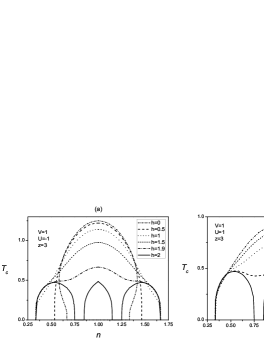
Figure 1: Phase diagram in the plane ($T,n$) for $V=1$ and $z=3$ and several values of $h$, and for (a) $U=-1$; (b) $U=1$.

In the plane $(n,T)$, for attractive $U$, the CO phase is observed in a interval $\Delta n$ which varies with the magnetic field. As it is shown in Fig. 1a, at $h=0$ and in the limit $T\to 0$, a complete CO state is established in the region $2/z\leq n\leq 2(z-1)/z$. $\Delta n$ first increases with $T$, then decreases vanishing at $n=1$, where the maximum critical temperature is reached; a reentrant behavior characterizes this region. Upon turning on a finite magnetic field, $\Delta n$ increases by increasing $h$ and the reentrant behavior is lost. For $h\geq|U|$, a CO state is established in the region $1/z\leq n\leq(2z-1)/z$ (in the limit $T\to 0$). The phase diagram still presents a single lobe structure centered at $n=1$, although the height of the lobe has decreased. There exists a critical value of the magnetic field $h_{T}=zV/2-U/2$ above which one observes the formation of three separated lobes centered around $n=0.5$, $n=1$ and $n=1.5$, respectively. The transition to the CO phase is suppressed in the range $0.75<n<0.85$ and $1.15<n<1.25$ (for $z=3$). By further increasing $h$, the central lobe shrinks and eventually disappears. As one can infer from Fig. 1b, the picture is very similar for repulsive on-site interaction. The phase diagram presents a single lobe structure centered at $n=1$: a CO phase is observed below the critical temperature in the range $1/z<n<(2z-1)/z$, which does not depend on $h$. At the same value of the magnetic field $h_{T}=zV/2-U/2$, the CO phase is observed inside the three separated lobes as for the case $U<0$. When plotted as a function of the magnetic field, the critical temperature shows a decreasing behavior, which is more pronounced in the neighborhood of $n=1$. Moreover, as one can also notice from Figs. 1, according to the value of the particle density, two situation can occur: either the transition temperature is finite for all values of $h$ or it vanishes at same critical value. In Fig. 2a, we plot the transition temperature $T_{c}$ as a function of the magnetic field at $n=0.75$, $z=3$ and for different values of the on-site potential. The transition temperature decreases by increasing $U$ and vanishes at $h_{T}=zV/2-U/2$. For $U=3V$, $h_{T}=0$: a strong on-site repulsion inhibits the CO phase, as already noticed in Ref. mancinis09 .

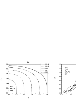
Figure 2: (a) The critical temperature $T_{c}$ as a function of the magnetic field $h$ at $n=0.75$ for $V=1$ and $z=3$, and several values of $U$. (b) The specific heat as a function of the temperature at $n=0.75$, for $V=1$, $U=-1$, and $z=3$, and several values of $h$.

The study of the specific heat also enlightens the influence of the magnetic field on the thermodynamic behavior of the system. The specific heat is given by $C=dE/dT$, where the internal energy $E$ can be computed as the thermal average of the Hamiltonian (1). As an example of the characteristic behavior of the specific heat by varying $h$, in Fig. 2b we plot $C$ as a function of the temperature at $U=-1$, $z=3$ and $n=0.75$, for several values of the magnetic field. For $h=0$ and at low temperatures, the system is in a CO phase and exhibits a phase transition at $T_{c}$ to a homogeneous phase. The specific heat exhibits a peak at $T_{1}=T_{c}$ - due to the phase transition - and another peak $T_{2}$ at low temperatures which vanishes as $h$ increases. For finite magnetic fields, the position of the peak $T_{1}$ and the relative height decrease by augmenting $h$. For $h=h_{T}$, the transition is suppressed and, correspondingly, the peak $T_{1}$ disappears.

The competition among the magnetic field and the on-site and intersite potentials gives rise to the formation of plateaus in the magnetization curves. By increasing the magnetic field, one observes plateaus whose starting points depend on the particle density, as well as on the on-site potential: one identifies two critical values of the magnetic field. The nonzero magnetization can either begin from $h=0$ or from a finite field. $h_{c}$ denotes the starting point of a nonzero magnetization, whereas $h_{s}$ denotes the value of the magnetic field when it reaches saturation.

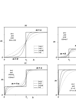
Figure 3: The magnetization $m$ as a function of the magnetic field $h$ at $T=0$.

The results for the magnetization $m(h)$ are shown in Fig. 3, where $U_{c}$ is the critical value of the on-site potential separating the different observed behaviors; for $z=3$, one finds $U_{c}\approx 2.8$. Making reference to Fig. 3 for the different regions of $n$ and $U$, one has: $h_{c}=h_{s}=|U|/2$ (Fig. 3a), $h_{c}=|U|/2$ and $h_{s}=zV/2+|U|/2$ (Fig. 3b), $h_{c}=0$ and $h_{s}=zV/2-U/2$ (Fig. 3c), and $h_{c}=h_{s}=0$ (Fig. 3d). The so-called metamagnetic behavior is clearly seen: at low temperatures the magnetization begins to show a typical $S$-shape which becomes more pronounced by further decreasing the temperature. At $T=0$ one, two or three plateaus ($m=0$, $m=1-n$ and $m=n$) are observed, according to the values of the external parameters. These results are similar to the ones obtained in one-dimensional AL-EHM mancini_epjb09 and spin-1 antiferromagnetic Ising chain with single-ion anisotropy chen03 ; mancini08 .

In Figs. 4a-b we plot the spin susceptibility as a function of the magnetic field at $T=0.1$ for several values of $U$ (both attractive and repulsive), $z=3$ and for $n=0.75$. In the limit $T\to 0$, the spin susceptibility diverges in correspondence of the values $h_{crit}$ at which the system moves from one magnetization plateau to the other. For low values of the magnetic field and attractive on-site interactions - corresponding to Fig. 4a - the spin susceptibility vanishes at low temperatures for all values of the filling: in the limit $T\to 0$ all electrons are paired and no alignment of the spin is possible. By increasing $h$, the magnetic excitations break some of the doublons inducing a finite magnetization: $\chi_{s}$ has a peak, then decreases, the system having entered the successive magnetic plateau. If $0.5<n<1$ then another peak is observed, corresponding to the second jump of the magnetization when $h$ reaches the saturated value $h_{s}$. On the other hand, for repulsive on-site interactions, a very small magnetic field induces a finite magnetization (with the exception of $n=1$ when $U<U_{c}$): $\chi_{s}$ has a maximum at $h=0$ and then decreases by augmenting $h$, unless another transition line is encountered, as it happens for $0.5<n\leq 1$ and $0<U<U_{c}$.

Figure 4: (a) The spin susceptibility as a function of the temperature for $V=1$, $n=0.75$, and (a) attractive (b) repulsive on-site interaction.

III Concluding remarks

The Green’s function and equations of motion formalism allows one to tackle a large class of classical fermionic and spin systems, providing a general formulation for any dimension and any underlying lattice Mancini05 ; mancini2 ; mancini05b ; mancini08 . In this paper we have evidenced how the use of this formalism leads to the exact solution of the AL-EHM on the Bethe lattice in the presence of an external magnetic field. By considering nearest-neighbor repulsion $V$, there is a transition temperature below which a charge ordered phase, characterized by a different distribution of the electrons in alternating shells, is established for $n>1/z$. The onset of the CO phase is signalled by the breaking of translational invariance: at $T_{c}$ the values of both the particle density and the double occupation become site or, more properly, shell dependent mancinis09 . The charge ordered phase is dramatically affected by the presence of a magnetic field: the transition temperature is lessen by a finite magnetic field. The CO phase shrinks by increasing $h$, leading to the appearance of large regions where the strength of the magnetic field prevents the ordering of the particles. By investigating the magnetic properties of the system, we found magnetic plateaus at low temperature. Furthermore, we identified the values of the critical fields $h_{c}$ and $h_{s}$, defining the beginning point of nonzero magnetization and the saturated magnetization field, respectively.

References

- (1) R. J. Baxter, Exactly Solvable Models in Statistical Mechanics, Academic Press, New York, 1982.
- (2) G. M. Dykes, J. Chem. Technol. Biotechnol. 76, 903 (2001).
- (3) F. Mancini, and F. P. Mancini, Eur. Phys. J. B 73, 581 (2010).
- (4) F. D. M. Haldane, Phys. Lett. A 93, 464 (1993); Phys. Rev. Lett. 50, 1153 (1983).
- (5) F. Mancini, and A. Avella, Adv. Phys. 53, 537 (2004) .
- (6) F. Mancini, Europhys. Lett. 70, 484 (2005).
- (7) F. Mancini, and F. P. Mancini, Phys. Rev. E 77, 061120 (2008).
- (8) F. Mancini, Eur. Phys. J. B 47, 527 (2005).
- (9) F. Mancini, and F. P. Mancini, Eur. Phys. J. B 68, 341 (2009).
- (10) X. Y. Chen, Q. Jiang, W. Z. Shen, and C. G. Zhong, Jour. Magn. Magn. Mat. 262, 258 (2003).
- (11) F. Mancini, and F. P. Mancini, Condens. Matter Phys. 11, 543 (2008).