Synthesis of the Optimal 4-bit Reversible Circuits

Abstract

Optimal synthesis of reversible functions is a non-trivial problem. One of the major limiting factors in computing such circuits is the sheer number of reversible functions. Even restricting synthesis to 4-bit reversible functions results in a huge search space (16! $\approx$ $2^{44}$ functions). The output of such a search alone, counting only the space required to list Toffoli gates for every function, would require over 100 terabytes of storage.

In this paper, we present an algorithm, that synthesizes an optimal circuit for any 4-bit reversible specification. We employ several techniques to make the problem tractable. We report results from several experiments, including synthesis of random 4-bit permutations, optimal synthesis of all 4-bit linear reversible circuits, synthesis of existing benchmark functions, and distribution of optimal circuits. Our results have important implications for the design and optimization of quantum circuits, testing circuit synthesis heuristics, and performing experiments in the area of quantum information processing.

1 Introduction

To the best of our knowledge, at present, physically reversible technologies are found only in the quantum domain [9]. However, “quantum” unites several technological approaches to information processing, including ion traps, optics, superconducting, spin-based and cavity-based technologies [9]. Of those, trapped ions [5] and liquid state NMR (Nuclear Magnetic Resonance) [10] are two of the most developed quantum technologies targeted for computation in the circuit model (as opposed to communication or adiabatic computing). These technologies allow computations over a set of 8 qubits and 12 qubits, correspondingly.

Reversible circuits are an important class of computations that need to be performed efficiently for the purpose of efficient quantum computation. Multiple quantum algorithms contain arithmetic units such as adders, multiplies, exponentiation, comparators, quantum register shifts and permutations, that are best viewed as reversible circuits. Moreover, reversible circuits are indispensable in quantum error correction [9]. Often, the efficiency of the reversible implementation is the bottleneck of a quantum algorithm (e.g., integer factoring and discrete logarithm [16]) or even a class of quantum circuits (e.g., stabilizer circuits [1]).

In this paper, we present an algorithm that finds optimal circuit implementations for 4-bit reversible functions. The algorithm has a number of potential uses and implications.

One major implication of this work is that it will help physicists with experimental design, since fore-knowledge of the optimal circuit implementation aids in the control over quantum mechanical systems. The control of quantum mechanical systems is very difficult, and as a result experimentalists are always looking for the best possible implementation. Having an optimal implementation helps to improve experiments or show that more control over a physical system needs to be established before a certain experiment could be performed.

A second important contribution is due to the efficiency of our implementation—$0.01$ seconds per synthesis of an optimal 4-bit reversible circuit. The algorithm could easily be integrated as part of peephole optimization, such as the one presented in [13].

Furthermore, our implementation allows us to propose a subset of optimal implementations that may be used to test heuristic synthesis algorithms. Currently, similar tests are performed by comparison to optimal 3-bit implementations. The best heuristic solutions have very tiny overhead, making such a test hard to improve. As such, it would help to replace this test with a more difficult one that allows more room for improvement.

Finally, due to the effectiveness of our approach, we are able to report new optimal implementations for small benchmark functions, approximate $L(4)$, the number of reversible gates required to implement a reversible 4-bit function, approximate the average number of gates required to implement a 4-bit permutation, and show the distribution of the number of permutations that may be implemented with $0..9$ gates.

2 Preliminaries

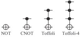
Figure 1: NOT, CNOT, Toffoli, and Toffoli-4 gates.

In this paper, we consider circuits with NOT, CNOT, Toffoli (TOF), and Toffoli-4 (TOF4) gates defined as follows:

• NOT$(a):\;a\mapsto a\oplus 1$;

• CNOT$(a,b):\;a,b\mapsto a,b\oplus a$;

• TOF$(a,b,c):\;a,b,c\mapsto a,b,c\oplus ab$;

• TOF4$(a,b,c,d):\;a,b,c,d\mapsto a,b,c,d\oplus abc$;

where $\oplus$ denotes an EXOR operation and concatenation is Boolean AND; see Figure 1 for illustration. These gates are used widely in quantum circuit construction, and have been demonstrated experimentally in multiple quantum information processing proposals [9]. In particular, CNOT is a very popular gate among experimentalists, frequently used to demonstrate control over a multiple-qubit quantum mechanical system. Since quantum circuits describe time evolution of a quantum mechanical system where individual “wires” represent physical instances, and time propagates from left to right, this imposes restrictions on the circuit topology. In particular, quantum and reversible circuits are strings of gates. As a result, feed-back (time wrap) is not allowed and there may be no fan-out (mass/energy conservation).

In this paper, we are concerned with searching for circuits requiring a minimal number of gates. Our focus is the proof of principle, i.e., showing that any optimal 4-bit reversible function may be synthesized efficiently, rather than attempting to report optimal implementations for a number of potentially plausible cost metrics. In fact, our implementation allows other circuit cost metrics to be considered, as discussed in Section 5.

In related work, there have been a few attempts to synthesize optimal reversible circuits with more than three inputs. Große et al. [3] employ SAT-based technique to synthesize provably optimal circuits for some small parameters. However, their implementation quickly runs out of resources. The longest optimal circuit they report contains 11 gates. The latter took 21,897.3 seconds to synthesize—same function that the implementation we report in this paper synthesized in .000106 seconds, see Table 6. Prasad et al. [13] used breadth first search to synthesize 26,000,000 optimal 4-bit reversible circuits with up to 6 gates in 152 seconds. We extend this search into finding 117,798,040,190 optimal circuits with up to 9 gates in 10,549 seconds. This is over 65 times faster and 4,500 times more than reported in [13]. Yang et al. [17] considered short optimal reversible 4-bit circuits composed with NOT, CNOT, and Peres [11] gates. They were able to synthesize optimal circuits for even permutations requiring no more than 12 gates. This amounts to approximately one quarter of the number of all 4-bit reversible functions. Our implementation allows optimal synthesis of any 4-bit reversible function, and it is much faster.

2.1 Motivating Example

Consider the two reversible circuit implementations in Figure 2 of a 1-bit full adder. This elementary function/circuit serves as a building block for constructing integer adders. The famous Shor’s integer factoring algorithm is dominated by adders like this. As such, the complexity of an elementary 1-bit adder circuit largely affects the efficiency of factoring an integer number with a quantum algorithm. It is thus important to have a well-optimized implementation of a 1-bit adder, as well as other similar small quantum circuit building blocks.

In this paper, we consider the synthesis of optimal circuits, i.e., we provably find the best possible implementation. Using optimal implementations of circuits potentially increases the efficiency of quantum algorithms and helps to reduce the difficulty with controlling quantum experiments.

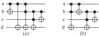
Figure 2: (a) a suboptimal and (b) an optimal circuit for 1-bit full adder.

3 Algorithm and Implementation

We first outline our algorithm and then discuss it in detail in the follow up subsections.

There are $N=2^{n}!$ reversible $n$-variable functions. The most obvious approach to the synthesis of all optimal implementations is to compute all optimal circuits and store them for later look-up. However, this is extremely inefficient. This is because such an approach requires $\Omega(N)$ space and, as a result, at least $\Omega(N)$ time. These space and time estimates are lower bounds, because, for instance, storing an optimal circuit requires more than a constant number of bits, but for simplicity, let us assume these figures are exact. Despite considering both figures for space and time unpractical, we use this simple idea as our starting point.

We first improve the space requirement by observing that if one synthesized all halves of all optimal circuits, then it is possible to search through this set to find both halves of any optimal circuit. It can be shown that the space requirement for storing halves has a lower bound of $\Omega(\sqrt{N})$. However, searching for two halves potentially requires a runtime on the order of the square of the search space, $\Omega\left((\sqrt{N})^{2}\right)=\Omega(N)$, a figure for runtime that we deemed inefficient. Our second improvement is thus to use a hash table to store the optimal halves. This reduces the runtime to soft $\Omega(\sqrt{N})$. While this lower bound does not necessarily imply that the actual complexity is lower than $O(N)$, this turns out to be the case, because the set of optimal halves is indeed much smaller than the set of all optimal circuits (an analytic estimate for the relative size of the former set is hard to obtain, though). Cumulatively, these two improvements reduce $\Omega(N)$ space and $\Omega(N)$ time requirement to $O(\#{\rm halves}(N))$ space and soft $O(\#{\rm halves}(N))$ time requirement. These reductions almost suffice to make the search possible using modern computers.

Our last step, apart from careful coding, that made the search possible is the reduction of the space requirement (with consequent improvement for runtime) by a constant of almost 48 via exploiting the following two features. First, simultaneous input/output relabeling, of which there are at most 24 (=4!) different ones, does not change the optimality of a circuit. And second, if an optimal circuit is found for a function $f$, an optimal circuit for the inverse function, $f^{-1}$, can be obtained by reversing the optimal circuit for $f$. This allows to additionally “pack” up to twice as many functions into one circuit. The cumulative improvement resulting from these two observations, is by a factor of almost $2\times 24=48$. Due to symmetries, the actual number is slightly less. See Table 4 (column 2 versus column 3) for exact comparison.

3.1 The search-and-lookup algorithm

For brevity, let the size of a reversible function mean the minimal number of gates required to implement it. Using breadth-first search, we can generate the smallest circuits for all reversible functions of size at most $k$, for a certain value of $k$. (This can be done in advance, on a larger machine, and need not be repeated for each reversible function.)

Assume that the given function $f$, for which we need to synthesize a minimal circuit, has size at most $2k$. We can first check whether $f$ is among the known functions of size at most $k$ and, if so, output the corresponding minimal circuit. If not, then the size of $f$ is between $k+1$ and $2k$, inclusive, and there exist reversible functions $g$ and $h$ of size $k$ and at most $k$, respectively, such that $f=h\circ g$. If we find such $g$ of the smallest size, then we can obtain the smallest circuit for $f$ by composing the circuits for $g$ and $h$.

Multiplying the above equality by $g^{-1}$, we obtain $f\circ g^{-1}=h$. Observe that $g^{-1}$ has the same size as $g$. Therefore, by trying all functions $g$ of size $1,2,\ldots,k$ until we find one such that $f\circ g$ has size $k$, we can find a $g$ of the smallest size.

The above algorithm involves sequential access to the functions of size at most $k$ and their minimal circuits and a membership test among functions of size $k$. Since the latter test must be fast and requires random memory access, we need to store all functions of size $k$ in memory. Thus, the amount of available RAM imposes an upper bound on $k$.

In practice, we store a 4-bit reversible function using a 64-bit word, because this allows for an efficient implementation of functional composition, inversion, and other necessary operations. On a typical PC with 4GB of RAM, we can store all functions for $k=6$. This means that we can apply the above search algorithm only to functions of size at most 12. Unfortunately, this will not cover all 4-bit reversible functions. Therefore, further reduction of memory usage is necessary.

3.2 Symmetries

A significant reduction of the search space can be achieved by taking into account the following symmetries of circuits:

1. Simultaneous relabeling of inputs and outputs. Given an optimal circuit implementing a 4-bit reversible function $f$ with inputs $x_{0},x_{1},x_{2},x_{3}$ and outputs $y_{0},y_{1},y_{2},y_{3}$ and a permutation $\sigma:\{0,1,2,3\}\to\{0,1,2,3\},$ we can construct a new circuit by relabeling the inputs and outputs into $x_{\sigma(0)},x_{\sigma(1)},x_{\sigma(2)},x_{\sigma(3)}\;{\rm and}\;y_{\sigma(0)},y_{\sigma(1)},y_{\sigma(2)},y_{\sigma(3)},$ respectively. Then the new circuit will provide a minimal implementation of the corresponding reversible function $f_{\sigma}$. Indeed, if it is not minimal and there is an implementation of $f_{\sigma}$ by a circuit with a smaller number of gates, we can relabel the inputs and outputs of this implementation with $\sigma^{-1}$ and obtain a smaller circuit implementing the original function $f$. This contradicts the assumption that the original circuit for $f$ is optimal.

   Given $f$ and $\sigma$, a formula for $f_{\sigma}$ can be easily obtained. Observe that the mapping $x_{0},x_{1},x_{2},x_{3}\mapsto x_{\sigma(0)},x_{\sigma(1)},x_{\sigma(2)},$ $x_{\sigma(3)}$ is a 4-bit reversible function, which we denote by $g_{\sigma}$. The mapping $y_{\sigma(0)},y_{\sigma(1)},y_{\sigma(2)},y_{\sigma(3)}\mapsto y_{0},y_{1},y_{2},y_{3}$ is then given by the inverse, $g_{\sigma}^{-1}$. Therefore, the four bit values $y_{0},y_{1},y_{2},y_{3}$ of $f_{\sigma}$ on a four-bit tuple $x_{0},x_{1},x_{2},x_{3}$ can be obtained by applying first $g_{\sigma}$, then $f$, and finally $g_{\sigma}^{-1}$. We obtain $f_{\sigma}=g_{\sigma}^{-1}\circ f\circ g_{\sigma}.$ We call the set of functions $f_{\sigma}$ the conjugacy class of $f$ modulo simultaneous input/output relabelings.

   Since there exist 24 permutations of 4 numbers, by choosing different permutations $\sigma$, we obtain 24 functions of the above form $f_{\sigma}$ for a fixed function $f$. Some of these functions may be equal, whence the size of the conjugacy class of $f$ may be smaller than 24. For example, if $f$=NOT$(a)$, then there exist only $4$ distinct functions of the form $f_{\sigma}$ (counting $f$ itself). Our experiments show, however, that for the vast majority of functions, the conjugacy classes are of size 24.

2. Inversion. As mentioned above, if we know a minimal implementation for $f$, then we know one for its inverse as well.

Note that conjugation and inversion commute:

$$(g_{\sigma}^{-1}\circ f\circ g_{\sigma})^{-1}=g_{\sigma}^{-1}\circ f^{-1}\circ g_{\sigma}.$$

For a function $f$, consider the union of the two conjugacy classes of $f$ and $f^{-1}$. Call the elements of this union equivalent to $f$. It follows that equivalent functions have the same size. Moreover, since gates are idempotent (i.e., equal to their own inverses) and their conjugacy classes consist of gates, if we know a minimal circuit for $f$, we can easily obtain one for any function in the equivalence class of $f$. Formally, if $f=g_{1}\circ\ldots\circ g_{n}$, where $n$ is the size of $f$ and $g_{i}$ are gates, then $f^{-1}=g_{n}\circ\ldots\circ g_{1}$, and if $f^{\prime}=g_{\sigma}^{-1}\circ f\circ g_{\sigma}$, then $f^{\prime}=g_{1}^{\prime}\circ\ldots\circ g_{n}^{\prime}$, where $g_{i}^{\prime}=g_{\sigma}^{-1}\circ g_{i}\circ g_{\sigma}$ are also gates. Our experiments show that a vast majority of functions have 48 distinct equivalent functions. This fact can reduce the search space by almost a factor of 48 as follows.

For a function $f$, define the canonical representative of its equivalence class. A convenient canonical representative can be obtained by introducing the lexicographic order on the set of 4-bit reversible functions, considered as permutations of $\{0,1,2,\ldots,15\}$ and encoded accordingly by the sequence $f(0),f(1),\ldots,f(15)$, and choosing the function whose corresponding sequence is lexicographically smallest. Now, instead of storing all functions of size at most $k$, store the canonical representative for each equivalence class. This will reduce the storage size by almost a factor of 48. Then, we use the Algorithm 1 to search for a minimal circuit for a given reversible function $f$.

Algorithm 1 Minimal circuit.

0:  Reversible function $f$ of size at most $L$.Hash table $H$ containing canonical representatives of all equivalence classes of functions of size at most $k$ and the last gates of their minimal circuits, $k\geq L/2$.Lists $A_{i}$, $1\leq i\leq L-k$, of all functions of size $i$.

0:  A minimal circuit $c$ for $f$.

  if $f=\;$IDENTITY then

     return  empty circuit

  end if

  $E_{f}\leftarrow$ equivalence class of $f$

  $\bar{f}\leftarrow$ canonical representative of $E_{f}$

  if $\bar{f}\in H$ then

     $\bar{\lambda}\leftarrow$ last gate of $\bar{f}$

     if $f$ is a conjugate of $\bar{f}$ then

        let $f=g_{\sigma}^{-1}\circ\bar{f}\circ g_{\sigma}$

        $\lambda\leftarrow g_{\sigma}^{-1}\circ\bar{\lambda}\circ g_{\sigma}$

        $c\leftarrow$ minimal circuit for $f\circ\lambda$

        return  $c\circ\lambda$

     else

        let $f=g_{\sigma}^{-1}\circ\bar{f}^{-1}\circ g_{\sigma}$

        $\lambda\leftarrow g_{\sigma}^{-1}\circ\bar{\lambda}\circ g_{\sigma}$

        $c\leftarrow$ minimal circuit for $\lambda\circ f$

        return  $\lambda\circ c$

     end if

  end if

  for $i=1$ to $L-k$ do

     for $g\in A_{i}$ do

        $h\leftarrow g\circ f$

        $E_{h}\leftarrow$ equivalence class of $h$

        $\bar{h}\leftarrow$ canonical representative of $E_{h}$

        if $\bar{h}\in H$ then

           $c_{g}\leftarrow$ minimal circuit for $g$

           $c_{h}\leftarrow$ minimal circuit for $h$

           return  $c_{g}^{-1}\circ c_{h}$

        end if

     end for

  end for

  return  error: size of $f$ is greater than $L$

The algorithm requires a hash table with canonical representatives of equivalence classes of size at most $k$, together with the last gates of their minimal circuits, and lists of all permutations of size at most $L-k$. We have pre-computed the canonical representatives for $k=9$ using breadth-first search (see Algorithm 2). For efficiency reasons, we store the last or the first gate of a minimal circuit for each canonical representative. However, this information is clearly sufficient to reconstruct the entire circuit and, in particular, the last gate. Using this pre-computed data, the hash table and the lists of all permutations of size at most $L-k$ are formed at the start-up. An implementation storing only the hash table is possible. Such an implementation will require less RAM memory, but it will be slower. We decided to focus on higher speed, because Table 3 indicates that we do not need to be able to search optimal circuits requiring up to 18 ($=9\times 2$) gates, which we could do otherwise by storing only the hash table.

Algorithm 2 Breadth-first search.

0:  $k$

0:  Lists $A_{i}$ of canonical representatives of size $\leq k$;Hash table $H$ with these canonical representatives and their first or last gates.

  Let $H$ be a hash table (keys are functions, values are gates)

  $H$.insert(IDENTITY, HAS_NO_GATES)

  $A_{0}\leftarrow\{{\rm IDENTITY}\}$

  for $i$ from $1$ to $k$ do

     for $f\in A_{i-1}\cup\{a^{-1}\;|\;a\in A_{i-1}\}$ do

        for all gates $\lambda$ do

           $h\leftarrow f\circ\lambda$

           $E_{h}\leftarrow$ equivalence class of $h$

           $\bar{h}\leftarrow$ canonical representative of $E_{h}$

           if $\bar{h}\not\in H$ then

              if $h$ is a conjugate of $\bar{h}$ then

                 let $h=g_{\sigma}^{-1}\circ\bar{h}\circ g_{\sigma}$

                 $H$.insert($\bar{h}$, $g_{\sigma}^{-1}\circ\lambda\circ g_{\sigma}$, IS_A_LAST_GATE)

              else

                 let $h=g_{\sigma}^{-1}\circ\bar{h}^{-1}\circ g_{\sigma}$

                 $H$.insert($\bar{h}$, $g_{\sigma}^{-1}\circ\lambda\circ g_{\sigma}$, IS_A_FIRST_GATE)

              end if

              $A_{i}$.insert($\bar{h}$)

           end if

        end for

     end for

  end for

The correctness of Algorithm 1 is proved as follows. Suppose first that the size of $f$ is at most $k$. The canonical representative $\bar{f}$ of its equivalence class will have the same size as $f$, so it will be found in the hash table $H$. Since $\bar{\lambda}$ is the last gate of a minimal circuit for $\bar{f}$, the size of $\bar{f}\circ\bar{\lambda}$ is one less than the size of $\bar{f}$. The function $f\circ\lambda$ (computed if $f$ is a conjugate of $\bar{f}$) or the function $\lambda\circ f$ (computed if $f$ is a conjugate of $\bar{f}^{-1}$) is equivalent to $\bar{f}\circ\bar{\lambda}$ and therefore also is of size one less than the size of $\bar{f}$. Therefore, the recursive call on that function will terminate and return a minimal circuit, which we can compose with $\lambda$ (at the proper side) to obtain a minimal circuit for $f$. The depth of recursion is equal to the size of $f$, and at each call we do one hash table lookup, one computation of the canonical representative, and one conjugation of a gate (the latter can be looked up in a small table). Thus, this part of the algorithm requires negligible time.

If the size of $f$ is greater than $k$, but does not exceed $L$, then $f=g_{f}\circ h$ for some $h$ of size $k$ and $g_{f}$ of size $i$, $1\leq i\leq L-k$. Then $g=g_{f}^{-1}\in A_{i}$. Once the inner for-loop encounters this $g$, it will return the minimal circuit for $f$, because both recursive calls are for functions of size at most $k$. For a function $f$ of size $s>k$, the number of iterations required to find the minimal circuit satisfies

$$\sum_{i=1}^{s-1-k}|A_{i}|<r\leq\sum_{i=1}^{s-k}|A_{i}|.$$

At each iteration, one canonical representative is computed and looked up in the hash table. Since the size of $A_{i}$ grows almost exponentially (see Table 4, left column), the search time will decrease almost exponentially, and the storage will increase exponentially, as $k$ increases. The timings for $k=8,9$ measured on two different systems are summarized in Table 1 (see Section 4 for machine details). The hash table loading and overall memory usage times were 119 seconds, 3.5GB ($k=8$) and 1111 seconds, 43.04GB ($k=9$).

Table 1: Average times of computing minimal circuits of sizes $0..14$ (in seconds).

Size $\setminus$ $k$	8 (CS2)	8 (CS1)	9 (CS1)
0	$5.10\times 10^{-7}$	$5.15\times 10^{-7}$	$5.15\times 10^{-7}$
1	$8.70\times 10^{-7}$	$8.80\times 10^{-7}$	$8.80\times 10^{-7}$
2	$1.26\times 10^{-6}$	$1.27\times 10^{-6}$	$1.27\times 10^{-6}$
3	$1.66\times 10^{-6}$	$1.69\times 10^{-6}$	$1.68\times 10^{-6}$
4	$2.07\times 10^{-6}$	$2.14\times 10^{-6}$	$2.14\times 10^{-6}$
5	$2.47\times 10^{-6}$	$2.52\times 10^{-6}$	$2.52\times 10^{-6}$
6	$3.48\times 10^{-6}$	$3.49\times 10^{-6}$	$3.96\times 10^{-6}$
7	$4.22\times 10^{-6}$	$4.11\times 10^{-6}$	$4.85\times 10^{-6}$
8	$4.49\times 10^{-6}$	$4.36\times 10^{-6}$	$4.45\times 10^{-6}$
9	$1.07\times 10^{-5}$	$1.18\times 10^{-5}$	$5.65\times 10^{-6}$
10	$2.28\times 10^{-4}$	$2.77\times 10^{-4}$	$1.79\times 10^{-5}$
11	$4.27\times 10^{-3}$	$5.20\times 10^{-3}$	$2.38\times 10^{-4}$
12	$6.30\times 10^{-2}$	$7.66\times 10^{-2}$	$3.74\times 10^{-3}$
13	$4.91\times 10^{-1}$	$5.98\times 10^{-1}$	$3.18\times 10^{-2}$
14	$4.38\times 10^{0}\;\,\,$	$5.33\times 10^{0}\;\,\,$	$3.26\times 10^{-1}$

It follows from the above complexity analysis that the performance of the following key operations affect the speed most:

• composition of two functions ($f\circ g$) and inverse of a function ($f^{-1}$),

• computation of the canonical representative of an equivalence class,

• hash table lookup.

In the next Subsection we discuss an efficient implementation of these operations.

3.3 Implementation details

As mentioned above, a 4-bit reversible function can be stored in a 64-bit word, by allocating 4 bits for each value of $f(0),f(1),\ldots,f(15)$. Then the composition of two functions can be computed in 94 machine instructions using the algorithm composition and the inverse function can be computed in 59 machine instructions using algorithm inverse.

unsigned64 composition(unsigned64 p, unsigned64 q) {
  unsigned64 d = (p & 15) << 2;
  unsigned64 r = (q >> p_i) & 15;
  p >>= 2; d = p & 60; r |= ((q >> d) & 15) << 4;
  p >>= 4; d = p & 60; r |= ((q >> d) & 15) << 8;
  p >>= 4; d = p & 60; r |= ((q >> d) & 15) << 16;
  ...
  p >>= 4; d = p & 60; r |= ((q >> d) & 15) << 60;
  return r;
}

unsigned64 inverse(unsigned64 p) {
  p >>= 2;
  unsigned64 q =  1 << (p & 60);
  p >>= 4;  q |=  2 << (p & 60);
  p >>= 4;  q |=  3 << (p & 60);
  ...
  p >>= 4;  q |= 15 << (p & 60);
  return q;
}

unsigned64 conjugate01(unsigned64 p) {
  p = (p & 0xF00FF00FF00FF00F)       |
     ((p & 0x00F000F000F000F0) << 4) |
     ((p & 0x0F000F000F000F00) >> 4);
  return (p & 0xCCCCCCCCCCCCCCCC)       |
        ((p & 0x1111111111111111) << 1) |
        ((p & 0x2222222222222222) >> 1);
}

In order to find the canonical representative in the equivalence class of a function $f$, we compute $f^{-1}$, generate all conjugates of $f$ and $f^{-1}$, and choose the smallest among the resulting 48 functions. Since every permutation of $\{0,1,2,3\}$ can be represented as a product of transpositions $(0,1)$, $(1,2)$, and $(2,3)$, the sequence of conjugates of $f$ by all 24 permutations can be obtained through conjugating $f$ by these transpositions. These conjugations can be performed in 14 machine instructions each as in function conjugate01.

Two functions can be compared lexicographically using a single unsigned comparison of the corresponding two words. Thus, the canonical representative can be computed using one inversion, $23\times 2=46$ conjugations by transpositions, and 47 comparisons, which totals to 750 machine instructions.

For the fast membership test, we use a linear probing hash table with Thomas Wang’s hash function [18] (see algorithm hash64shift).

long hash64shift(long key)
{
  key = (~key) + (key << 21); // signed shift
  key = key ^ (key >>> 24);   // unsigned shift
  key = (key + (key << 3)) + (key << 8);
  key = key ^ (key >>> 14);
  key = (key + (key << 2)) + (key << 4);
  key = key ^ (key >>> 28);
  key = key + (key << 31);
  return key;
}

This function is well suited for our purposes: it is fast to compute and distributes the permutations uniformly over the hash table. The parameters of the hash tables storing the canonical representatives of equivalence classes of size $k$, for $k=7,8,9$ are shown in Table 2.

Table 2: Parameters of linear hash tables storing canonical representatives.

$k$	7	8	9
Size	$2^{25}$	$2^{28}$	$2^{32}$
Memory Usage	256 MB	2 GB	32 GB
Load Factor	0.58	0.84	0.51
Average Chain Length	3.14	9.18	2.63
Maximal Chain Length	92	754	86

4 Performance and Results

We performed several tests using two computer systems, $CS1$ and $CS2$. $CS1$ is a high performance server with 16 AMD Opteron 2300 MHz processors, 64 GB RAM, and Seagate Barracuda ES2 SCSI 7200 RPM HDD running Linux. $CS2$ is a laptop Sony VGN-NS190D with Intel Core Duo 2000 GHz processor, 4 GB RAM, and a 5400 RPM SATA HDD running Linux. The following subsections summarize the tests and results.

4.1 Synthesis of Random Permutations

Table 3: Distribution of the number of gates required for 10,000,000 random 4-bit reversible functions.

Size	Functions
14	17,191
13	2,371,039
12	5,110,943
11	2,051,507
10	392,108
9	50,861
8	5,269
7	455
6	24
5	3

In this test, we generated 10,000,000 random uniformly distributed permutations using the Mersenne twister random number generator [7]. The test was executed on $CS1$. It took 104,616.716 seconds (about 29 hours) of user time and the maximal RAM memory usage was 43.04GB. Note that 1111 seconds (approximately 18 minutes) were spent loading previously computed optimal circuits with up to 9 gates (see Subsection 4.2 for details) into RAM. On average, it took only 0.01035 seconds to synthesize an optimal circuit for a permutation. The distribution of the circuit sizes is shown in Table 3.

Note, that the ratio of the number of random permutations requiring 9 gates to the number of all random permutations, $\frac{50,861}{10M}\approx.005086$, is close to the ratio of the number of all permutations requiring 9 gates to the number of all permutations, $\frac{105,984,823,653}{16!}\approx.005066$. This implies that the weighted average over the random sample, equal to $11.94$ gates per circuit, must be close to the actual weighted average. We further use this random sample and the results of the optimal 3-bit circuit synthesis [15] to approximate the number of permutations requiring 10 through 17 gates, see Table 4.

We conjecture that there are no permutations requiring 17 gates, and unlikely many, if at all, that require 16 gates. This implies that our search may be performed on a machine capable of storing reduced optimal implementations with up to 8 gates, i.e., a machine with 4GB RAM. Further analysis suggests that the search for an optimal circuit will complete in the majority of cases (99.999$\%$ assuming uniform distribution) if one uses optimal circuits with at most 7 gates and stores only the hash table. Such a search requires slightly more than 256M of available RAM, and could be executed on an older machine.

4.2 Distribution of Optimal Implementations

Table 4: Number of 4-bit permutations requiring 0..9 gates, and estimates of the number of permutations requiring 10..17 gates. Note, we were not able to estimate the number of functions for size 15 and 16.

Size	Functions	Reduced
		Functions
$\geq$17	0
16	???
15	???
14	$\sim 3.60\times 10^{10}$
13	$\sim 4.96\times 10^{12}$
12	$\sim 1.07\times 10^{13}$
11	$\sim 4.29\times 10^{12}$
10	$\sim 8.20\times 10^{11}$
9	105,984,823,653	2,208,511,226
8	10,804,681,959	225,242,556
7	932,651,938	19,466,575
6	70,763,560	1,482,686
5	4,807,552	101,983
4	294,507	6,538
3	16,204	425
2	784	33
1	32	4
0	1	1

Table 4 lists the distribution of the number of permutations that can be realized with optimal circuits requiring no more than 9 gates. We estimate the number of functions requiring $10..17$ gates using random function size distribution, see Table 3, and optimal synthesis of all 3-bit reversible functions. We used $CS1$ to run this test, and it took 10,549 seconds (under 3 hours) to complete using 43.04 GB of RAM. $CS2$ used 2.74 GB RAM and took 743.401 seconds (under 13 minutes) to synthesize optimal implementations with up to 8 gates.

4.3 Optimal linear circuits

Table 5: Number of 4-bit linear reversible functions requiring 0..10 gates in an optimal implementation.

Size	Functions
10	138
9	13555
8	84225
7	118424
6	72062
5	26182
4	6589
3	1206
2	162
1	16
0	1

Linear reversible circuits are the most complex part of error correcting circuits [1]. Efficiency of these circuits defines efficiency of quantum encoding and decoding error correction operations. Linear reversible functions are those whose positive polarity Reed-Muller polynomial has only linear terms. More simply, linear reversible functions are those computable by circuits with NOT and CNOT gates.

For example, the reversible mapping $a,b,c,d\mapsto b\oplus 1,a\oplus c\oplus 1,d\oplus 1,a$ is a linear reversible function. Interestingly, this linear function is one of the 138 most complex linear reversible functions—it requires 10 gates in an optimal implementation. The optimal implementation of this function is given by the circuit CNOT(b,a) CNOT(c,d) CNOT(d,b) NOT(d) CNOT(a,b) CNOT(d,c) CNOT(b,d) CNOT(d,a) NOT(d) CNOT(c,b).

We synthesized optimal circuits for all 322,560 4-bit linear reversible functions. This process took under two seconds on $CS2$. The distribution of the number of functions requiring a given number of gates is shown in Table 5.

4.4 Synthesis of Benchmarks

Table 6: Optimal implementations of benchmark functions.

Name	Specification	SBKC	Source	PO?	SOC	Our optimal circuit	Runtime
4_49	[15,1,12,3,5,6,8,7,	12	[6]	No	12	NOT(a) CNOT(c,a) CNOT(a,d) TOF(a,b,d)	.000690s
	0,10,13,9,2,4,14,11]					CNOT(d,a) TOF(c,d,b) TOF(a,d,c) TOF(b,c,a)
						TOF(a,b,d) NOT(a) CNOT(d,b) CNOT(d,c)
4bit-7-8	[0,1,2,3,4,5,6,8,7,9,	7	[8]	No	7	CNOT(d,b) CNOT(d,a) CNOT(c,d) TOF4(a,b,d,c)	.000003s
	10,11,12,13,14,15]					CNOT(c,d) CNOT(d,b) CNOT(d,a)
decode42	[1,2,4,8,0,3,5,6,7,9,	11	[4]	No	10	CNOT(c,b) CNOT(d,a) CNOT(c,a) TOF(a,d,b)	.000006s
	10,11,12,13,14,15]					CNOT(b,c) TOF4(a,b,c,d) TOF(b,d,c)
						CNOT(c,a) CNOT(a,b) NOT(a)
hwb4	[0,2,4,12,8,5,9,11,1,	11	[6]	Yes	11	CNOT(b,d) CNOT(d,a) CNOT(a,c) TOF4(b,c,d,a)	.000106s
	6,10,13,3,14,7,15]					CNOT(d,b) CNOT(c,d) TOF(a,c,b) TOF4(b,c,d,a)
						CNOT(d,c) CNOT(a,c) CNOT(b,d)
imark	[4,5,2,14,0,3,6,10,	7	[13]	No	7	TOF(c,d,a) TOF(a,b,d) CNOT(d,c) CNOT(b,c)	.000003s
	11,8,15,1,12,13,7,9]					CNOT(d,a) TOF(a,c,b) NOT(c)
mperk	[3,11,2,10,0,7,1,6,	9*	[12, 8]	No	9	NOT(c) CNOT(d,c) TOF(c,d,b) TOF(a,c,d)	.000003s
	15,8,14,9,13,5,12,4]					CNOT(b,a) CNOT(d,a) CNOT(c,a) CNOT(a,b)
						CNOT(b,c)
oc5	[6,0,12,15,7,1,5,2,4,	15	[14]	No	11	TOF(b,d,c) TOF(c,d,b) TOF(a,b,c) NOT(a)	.000313s
	10,13,3,11,8,14,9]					CNOT(d,b) CNOT(a,c) TOF(b,c,d) CNOT(a,b)
						CNOT(c,a) CNOT(a,c) TOF4(a,b,d,c)
oc6	[9,0,2,15,11,6,7,8,	14	[14]	No	12	TOF4(b,c,d,a) TOF4(a,c,d,b) CNOT(d,c) TOF(b,c,d)	.000745s
	14,3,4,13,5,1,12,10]					TOF(c,d,a) TOF4(a,b,d,c) CNOT(b,a) NOT(a)
						CNOT(c,b) CNOT(d,c) CNOT(a,d) TOF(b,d,c)
oc7	[6,15,9,5,13,12,3,7,	17	[14]	No	13	TOF(b,d,c) TOF(a,b,d) CNOT(b,a) TOF4(a,c,d,b)	.0265s
	2,10,1,11,0,14,4,8]					CNOT(c,b) CNOT(d,c) TOF(a,c,d) NOT(b) NOT(d)
						CNOT(b,c) TOF(b,d,a) TOF(a,c,d) CNOT(c,a)
oc8	[11,3,9,2,7,13,15,14,	16	[14]	No	12	CNOT(d,a) TOF(b,c,a) TOF(c,d,b) TOF4(a,b,d,c)	.001395s
	8,1,4,10,0,12,6,5]					TOF(a,b,d) TOF(a,d,b) NOT(a) NOT(b)
						TOF(b,d,a) CNOT(a,d) TOF(b,c,d)
primes4	[2,3,5,7,11,13,0,1,4,	N/A	N/A	N/A	10	CNOT(d,c) CNOT(c,a) CNOT(b,c) NOT(b)	.000012s
	6,8,9,10,12,14,15]					TOF(b,c,d) TOF4(a,b,d,c) TOF(a,c,b)
						NOT(a) TOF4(a,c,d,b) CNOT(b,a)
rd32	[0,7,6,9,4,11,10,13,	4	[2]	Yes	4	TOF(a,b,d) CNOT(a,b) TOF(b,c,d) CNOT(b,c)	.000002s
	8,15,14,1,12,3,2,5]
shift4	[1,2,3,4,5,6,7,8,9,	4	[8]	Yes	4	TOF4(a,b,c,d) TOF(a,b,c) CNOT(a,b) NOT(a)	.000002s
	10,11,12,13,14,15,0]

In this subsection, we present optimal circuits for benchmark functions that have been previously reported in the literature. Table 6 summarizes the results. The table describes the Name of the benchmark function, its complete Specification, Size of the Best Known Circuit (SBKC), the Source of this circuit, indicator of whether this circuit has been Proved Optimal (PO?), Size of an Optimal Circuit (SOC), the optimal implementation that our program found, and the runtime our program takes to find this optimal implementation. We used $CS1$ for this test, and report the runtime it takes after hash table with all optimal implementations with up to 9 gates is loaded into RAM. Shorter runtimes were identified using multiple runs of the search to achieve sufficient accuracy. Please note that we introduce the function $primes4$, which cannot be found in previous literature. Also, the 9-gate circuit for function mperk requires some extra SWAP gates to properly map inputs into their respective outputs, indicated by an asterisk.

4.5 Searching for a Hard Permutation

We executed a 12-hour search using $CS1$ to find a permutation requiring more than 14 gates in an optimal implementation. To run the search, we used 14- and 13- gate optimal implementations and tried to extend them by assigning gates to the beginning and the end of those optimal implementations, computing the resulting function, and verifying how many gates they require. After the 12 hour search, we were not able to find a permutation requiring more than 14 gates, indicating further that there are not many such permutations.

5 Conclusions and Future Work

In this paper, we described an algorithm that finds an optimal circuit for any 4-bit reversible function. Our goal was to minimize the number of gates required for function implementation. Our program implementation takes approximately 3 hours to calculate all optimal implementations requiring up to 9 gates, and then an average of about $0.01$ seconds to search for an optimal circuit of any 4-bit reversible function. Both calculations are surprisingly fast given the size of the search space.

We demonstrated the synthesis of 117,798,040,190 optimal circuits in 10,549 seconds, amounting to an average speed of 11,166,749 circuits per second. This is over 65 times faster and some 4,500 times more than the best previously reported result (26 million circuits in 152 seconds) [13]. We synthesized optimal implementations for all linear reversible functions.

We also demonstrated that the search for an optimal circuit can be done very quickly. For example, if all optimal circuits are written to a hypothetical 100+TB 5400 RPM hard drive, the average time to extract a random circuit from the drive would be expected to take on the order of $0.01-0.02$ seconds (typical access time for 5400 RPM hard drives). In other words, it would likely take longer to read the answer from a hypothetical hard drive than to compute it with our implementation. Furthermore, the 3-hour calculation of all optimal circuits with up to 9 gates could be reduced by storing its result (computed once for the entirety of the described search and its follow up executions) on the hard drive, as was done in Subsection 4.1. It took 1111 seconds, i.e., under 18 minutes, to load optimal circuits with up to 9 gates into RAM using $CS1$. Given that the media transfer rate of modern hard drives is 1Gbit/s (=1GB in 8 seconds) and higher, it may take no longer than 5 minutes ($=300$s $>296=37*8$s) to load optimal implementations into RAM to initiate the search on a different machine.

Minor modifications to the algorithm could be explored to address other optimization issues. For example, for practicality, one may be interested in minimizing depth. This may be important if a faster circuit is preferred, and/or if quantum noise has a stronger constituent with time, than with the disturbance introduced by multiple gate applications. It may also be important to account for the different implementation costs of the gates used (generally, NOT is much simpler than CNOT, which in turn, is simpler than Toffoli). Both modifications are possible, by making changes only to the first part of the search.

To optimize depth, one needs to consider a different family of gates, where, for instance, sequence NOT$(a)\;$CNOT$(b,c)$ is counted as a single gate. To account for different gate costs, one needs to search for small circuits via increasing cost by one (assuming costs are given as natural numbers), as opposed to adding a gate to all maximal size optimal circuits.

It is also possible to extend the search to find optimal implementations in restricted architectures (trivially if an optimal implementation is required up to the input/output permutation). Finally, the search could be extended to find some small optimal 5-bit circuits. However, more work is necessary to determine how far the search progress could be carried with 5-bit optimal implementations.

Our future plans include:

• execution of an extended search to find a hard permutation, one requiring a large ($\geq 15$) number of gates;

• construction of a representative set of functions that could be used to test heuristic synthesis algorithms against;

• computing all numbers in Table 4 exactly. If completed, this automatically solves the first task by appropriately keeping track of relevant computations. Also, this would give an exact number for $L(4)$, the maximal number of gates required to implement a 4-bit reversible function, and help with the second task;

• finding depth-optimal 4-bit circuits and optimal 5-bit circuits. In particular, a simple calculation shows that using $CS1$ it is possible to compute all optimal 5-bit circuits with up to six gates, and thus it is possible to search optimal 5-bit implementations with up to 12 gates;

• extending techniques reported in this paper to the synthesis of optimal stabilizer circuits. Coupled with peep-hole optimization algorithm for circuit simplification, these results may become a very useful tool in optimizing error correction circuits. This may be of a particular practical interest since implementations of quantum algorithms may be expected to be dominated by error correction circuits.

6 Acknowledgments

We wish to thank Dr. Donny Cheung from the University of Calgary for his useful discussions. We wish to thank Dr. Barry Schneider from the National Science Foundation for giving us access to his computer, named $CS1$ in our paper.

This article was based on work partially supported by the National Science Foundation, during D. Maslov’s assignment at the Foundation. Any opinion, finding and conclusions or recommendations expressed in this material are those of the author and do not necessarily reflect the views of the National Science Foundation.

References

- [1] S. Aaronson and D. Gottesman. Improved simulation of stabilizer circuits. Physical Review A, 70(052328), 2004, quant-ph/0406196.
- [2] R. P. Feynman. Quantum mechanical computers. Foundations of Physics, 16(6):507–531, June 1986.
- [3] D. Große, et al. Exact SAT-based Toffoli network synthesis. Proc. 17th ACM Great Lakes Symp. on VLSI, 2007.
- [4] P. Gupta, et al. An algorithm for synthesis of reversible logic circuits. IEEE TCAD, 25(11):2317–2330, November 2006.
- [5] H. Häffner, et al. Scalable multiparticle entanglement of trapped ions. Nature 438:643–646, December 2005, quant-ph/0603217.
- [6] D. Maslov. Reversible logic synthesis benchmarks page. http://webhome.cs.uvic.ca/~dmaslov/, May 2009.
- [7] M. Matsumoto and T. Nishimura. Mersenne twister: a 623-dimensionally equidistributed uniform pseudo-random number generator. ACM Trans. MCS, 8(1):3–30, 1998.
- [8] D. M. Miller. Spectral and two-place decomposition techniques in reversible logic. MWSCAS, August 2002.
- [9] M. Nielsen and I. Chuang. Quantum Computation and Quantum Information. Cambridge University Press, 2000.
- [10] C. Negrevergne, et al. Benchmarking Quantum Control Methods on a 12-Qubit System. Phys. Rev. Lett., 96, 170501, 2006, quant-ph/0603248.
- [11] A. Peres. Reversible logic and quantum computers. Phys. Rev. A, 32(6):3266 -3276, 1985.
- [12] M. Perkowski et al. A general decomposition for reversible logic. Proc. 5th Reed-Muller Workshop, pages 119–138, 2001.
- [13] A. K. Prasad, et al. Algorithms and data structures for simplifying reversible circuits. ACM JETC, 2(4), 2006.
- [14] M. Saeedi, et al. On the Behavior of Substitution-based Reversible Circuit Synthesis Algorithms: Investigation and Improvement. IEEE ISVLSI, pages 428–436, March 2007.
- [15] V. V. Shende, et al. Synthesis of Reversible Logic Circuits. IEEE TCAD, 22(6):710–722, June 2003, quant-ph/0207001.
- [16] P. W. Shor. Polynomial-time algorithms for prime factorization and discrete logarithms on a quantum computer. SIAM J. of Computing, 26:1484–1509, 1997.
- [17] G. Yang, et al. Bi-Directional Synthesis of 4-Bit Reversible Circuits. Computer J., 51(2):207–215, March 2008.
- [18] T. Wang. Integer Hash Function. Version 3.1, March 2007. http://www.concentric.net/Ttwang/tech/inthash.htm