Multisource Self-calibration for Sensor Arrays

Abstract

Calibration of a sensor array is more involved if the antennas have direction dependent gains and multiple calibrator sources are simultaneously present. We study this case for a sensor array with arbitrary geometry but identical elements, i.e. elements with the same direction dependent gain pattern. A weighted alternating least squares (WALS) algorithm is derived that iteratively solves for the direction independent complex gains of the array elements, their noise powers and their gains in the direction of the calibrator sources. An extension of the problem is the case where the apparent calibrator source locations are unknown, e.g., due to refractive propagation paths. For this case, the WALS method is supplemented with weighted subspace fitting (WSF) direction finding techniques. Using Monte Carlo simulations we demonstrate that both methods are asymptotically statistically efficient and converge within two iterations even in cases of low SNR.

I Introduction

In this paper we study the calibration of the direction dependent response of sensor array antennas, excited by simultaneously present calibrator sources. The antenna array has arbitrary geometry but identical antennas. The calibration involves the complex gain of the antenna elements towards each source. The source powers are known but we will allow for small deviations in apparent source locations to account for, e.g., refractive propagation paths. This problem is one of the main challenges currently faced in the field of radio astronomy. For low frequency observations ($<$ 300 MHz) this community is building or developing a number of new instruments, for example the low frequency array (LOFAR) [1], the Murchison wide field array (MWA) [2] and the primeval structure telescope (PaST) [3], which are all large irregular phased arrays. These difficulties arise due to the influence of the ionosphere on the propagation of radio waves, which can qualitatively be categorized into the following four regimes depending on the field of view (FOV) of the individual receptors and the baselines between them [4]:

Figure 1: Graphical representation of regime 3: all lines of sight towards a single source sample the same ionosphere, but the ionospheric delay differs per source due to the large FOV and short baselines (after [4]).

1. All antennas and all lines of sight sample the same ionospheric delays, thus the ionosphere causes no distortion of the array manifold (small FOV, short baselines).

2. Lines of sight from different antennas sample different ionospheric patches, but all sources in the antenna FOV experience the same delay; the ionosphere thus causes an antenna based gain effect (small FOV, long baselines).

3. All lines of sight towards a single source sample the same ionosphere but the delay differs per source. This regime requires source based direction dependent calibration (large FOV, short baselines, see Fig. 1).

4. The ionospheric delays differ per station and per source (large FOV, long baselines).

The first two regimes can be handled under the self-calibration assumption used in astronomy that all errors are telescope based thereby reducing the estimation problem to a single direction independent gain factor per telescope [5]. The problem of estimating these direction independent gains based on a single calibrator source is treated in [6], while the multiple source case has been discussed in [7]. The problem of finding a complex gain per antenna per source, the fourth regime, is not tractable without further assumptions which allow to parameterize the behavior of the gains over space, time and/or frequency [8]. In this paper we will focus on the third regime, which is sketched in Fig. 1, thus filling the gap in the available literature. It allows for the calibration of individual closely packed groups of antennas such as a LOFAR station or a subarray of the MWA and PaST telescopes and thus forms a valuable step towards the calibration of the whole array.

We will state our problem in general terms, since the problem plays a role in a range of applications varying from underwater acoustics to antenna arrays. This explains the persistent interest in on-line calibration, autocalibration or self-calibration of sensor arrays [9, 10, 11, 12, 8]. In most applications the main driver for studies on array calibration is to improve the DOA estimation accuracy. Many studies in this field therefore try to solve for the DOAs and a number of array parameters. In [13, 14, 9] self-calibration schemes are presented which solve for the direction independent gains and the sensor positions, i.e. the directional response of the sensors is assumed known. Other studies assume a controlled environment to calibrate the array by measuring the calibrator sources one at a time [15, 16] or exploit the array geometry, e.g. a uniform linear array (ULA) having a Toeplitz matrix as array covariance matrix [10, 17]. Weiss and Friedlander [18] have presented a technique for almost fully blind signal estimation. Their work, however, focuses on estimation and separation of source signals, not on characterizing the array itself. We thus feel that the problem at hand also forms an interesting addition to the literature available on sensor array calibration in general.

In the next section we introduce the data model and provide a mathematical formulation of the problem. In Sec. III the Cramèr-Rao bound for this estimation problem is discussed. Section IV presents an alternating least squares (ALS) and a weighted alternating least squares (WALS) approach optimizing subsets of parameters iteratively. These algorithms are validated using Monte Carlo simulations in Sec. V. The conclusions are drawn in Sec. VI.

Notation: Overbar $\overline{(\cdot)}$ denotes conjugation, the transpose operator is denoted by ^T, the complex conjugate (Hermitian) transpose by ^H and the pseudo-inverse by ^†. An estimated value is denoted by $\mathcal{E}\{\cdot\}$. $\odot$ is the element-wise matrix multiplication (Hadamard product), $\oslash$ is the element-wise matrix division, $\otimes$ denotes the Kronecker product and $\circ$ is used to denote the Khatri-Rao or column-wise Kronecker product of two matrices. $\mathrm{diag}(\cdot)$ converts a vector to a diagonal matrix with the vector placed on the main diagonal, $\mathrm{vecdiag}(\cdot)$ produces a vector from the elements of the main diagonal of its argument and $\mathrm{vec}(\cdot)$ converts a matrix to a vector by stacking the columns of the matrix. We exploit many properties of Kronecker products, including the following (for matrices and vectors of compatible dimensions):

$$\mathrm{vec}(\mathbf{A}\mathbf{B}\mathbf{C}) = (\mathbf{C}^{T}\otimes\mathbf{A})\mathrm{vec}(\mathbf{B})$$ (1)

$$\mathrm{vec}(\mathbf{A}\mathrm{diag}(\mathbf{b})\mathbf{C}) = (\mathbf{C}^{T}\circ\mathbf{A})\mathbf{b}$$ (2)

$$(\mathbf{A}\circ\mathbf{B})^{H}(\mathbf{C}\circ\mathbf{D}) = \mathbf{A}^{H}\mathbf{C}\odot\mathbf{B}^{H}\mathbf{D}$$ (3)

II Data model

We consider an array of $p$ elements located at a single site (“Regime 3”). Denote the complex baseband output signal of the $i$th array element by $x_{i}(t)$ and define the array signal vector $\mathbf{x}(t)=[x_{1}(t),x_{2}(t),\cdots,x_{p}(t)]^{T}$. We assume the presence of $q$ mutually independent i.i.d. Gaussian signals $s_{k}(t)$ impinging on the array, which are stacked in a $q\times 1$ vector $\mathbf{s}(t)$. Likewise the sensor noise signals $n_{i}(t)$ are assumed to be mutually independent i.i.d. Gaussian signals and are stacked in a $p\times 1$ vector $\mathbf{n}(t)$. If the narrow band condition holds [19], we can define the $q$ spatial signature vectors $\mathbf{a}_{k}$ ($p\times 1)$, which describe for the $k$th source the phase delays at each antenna due only to the geometry.

The $q$ sources are considered calibrator sources, thus we assume that their powers, their nominal positions, and the locations of the antennas (hence $\mathbf{a}_{k}$) are known. Refractive effects caused by ionospheric phase gradients may shift the apparent locations of the sources, thus we will also consider cases where the $\mathbf{a}_{k}$ are only parametrically known.

The sensors are assumed to have the same direction dependent gain behavior towards the $q$ source signals received by the array. This can include the antenna pattern and ionospheric phase effects. They are described by gain factors $g_{0k}$ and are collected in a matrix $\mathbf{G_{0}}=\mathrm{diag}([g_{01},g_{02},\cdots,g_{0q}])$. The direction independent gains and phases (individual receiver gains) can be described as ${\mbox{\boldmath{$\gamma$}}}=[\gamma_{1},\gamma_{2},\cdots,\gamma_{p}]^{T}$ and ${\mbox{\boldmath{$\phi$}}}=[\mathrm{e}^{\mathrm{j}\phi_{1}},\mathrm{e}^{\mathrm{j}\phi_{2}},\cdots,\mathrm{e}^{\mathrm{j}\phi_{p}}]^{T}$ respectively with corresponding diagonal matrix forms ${\mbox{\boldmath{$\Gamma$}}}=\mathrm{diag}({\mbox{\boldmath{$\gamma$}}})$ and ${\mbox{\boldmath{$\Phi$}}}=\mathrm{diag}({\mbox{\boldmath{$\phi$}}})$. With these definitions, the array signal vector can be described as

$$\mathbf{x}(t)={\mbox{\boldmath{$\Gamma$}}}{\mbox{\boldmath{$\Phi$}}}\left(\sum_{k=1}^{q}\mathbf{a}_{k}g_{0k}s_{k}(t)\right)+\mathbf{n}(t)=\mathbf{G}\mathbf{A}\mathbf{G}_{0}\mathbf{s}(t)+\mathbf{n}(t)$$ (4)

where $\mathbf{A}=[\mathbf{a}_{1},\cdots,\mathbf{a}_{k}]$ (size $p\times q$) and $\mathbf{G}={\mbox{\boldmath{$\Gamma$}}}{\mbox{\boldmath{$\Phi$}}}$; for later use we also define $\mathbf{g}={\mbox{\boldmath{$\gamma$}}}\odot{\mbox{\boldmath{$\phi$}}}$.

The signal is sampled with period $T$ and $N$ sample vectors are stacked into a data matrix $\mathbf{X}=[\mathbf{x}(T),\mathbf{x}(2T),\cdots,\mathbf{x}(NT)]$. The covariance matrix of $\mathbf{x}(t)$ is $\mathbf{R}=\mathcal{E}\{\mathbf{x}(t)\mathbf{x}^{H}(t)\}$ and is estimated by $\widehat{\mathbf{R}}=N^{-1}\mathbf{X}\mathbf{X}^{H}$. Likewise, the source signal covariance ${\mbox{\boldmath{$\Sigma$}}}_{s}=\mathrm{diag}({\mbox{\boldmath{$\sigma$}}}_{s})$ where ${\mbox{\boldmath{$\sigma$}}}_{s}=[\sigma_{s1}^{2},\sigma_{s2}^{2},\cdots,\sigma_{sq}^{2}]^{T}$ and the noise covariance matrix is ${\mbox{\boldmath{$\Sigma$}}}_{n}=\mathrm{diag}({\mbox{\boldmath{$\sigma$}}}_{n})$ where ${\mbox{\boldmath{$\sigma$}}}_{n}=[\sigma_{n1}^{2},\sigma_{n2}^{2},\cdots,\sigma_{np}^{2}]^{T}$. Then the model for $\mathbf{R}$ based on (4) is

$$\mathbf{R}=\mathbf{G}\mathbf{A}\mathbf{G}_{0}{\mbox{\boldmath{$\Sigma$}}}_{s}\mathbf{G}_{0}^{H}\mathbf{A}^{H}\mathbf{G}^{H}+{\mbox{\boldmath{$\Sigma$}}}_{n}.$$ (5)

In this model, ${\mbox{\boldmath{$\Sigma$}}}_{s}$ is known. Since $\mathbf{G}_{0}$ and ${\mbox{\boldmath{$\Sigma$}}}_{s}$ are diagonal matrices, we can introduce

$$\Sigma = \mathbf{G}_{0}{\mbox{\boldmath{$\Sigma$}}}_{s}\mathbf{G_{0}}^{H}$$ (6)

$$= \mathrm{diag}([|g_{01}|^{2}\sigma_{s1}^{2},\cdots,|g_{0q}|^{2}\sigma_{sq}^{2}])=\mathrm{diag}({\mbox{\boldmath{$\sigma$}}})\,.$$

Since the direction dependent gains $g_{0k}$ are not known, the real valued elements of ${\mbox{\boldmath{$\sigma$}}}=[\sigma_{1}^{2},\sigma_{2}^{2},\cdots,\sigma_{q}^{2}]^{T}$ are not known either. This implies that our problem is identical to estimating an unknown diagonal signal covariance matrix without any DOA dependent errors. We may thus restate (5) as

$$\mathbf{R}=\mathbf{G}\mathbf{A}{\mbox{\boldmath{$\Sigma$}}}\mathbf{A}^{H}\mathbf{G}^{H}+{\mbox{\boldmath{$\Sigma$}}}_{n}$$ (7)

and solve for $\mathbf{G}$, $\Sigma$ and ${\mbox{\boldmath{$\Sigma$}}}_{n}$ under the assumption that $\mathbf{A}$ is known (or parametrically known).

The data model described by (7) is commonly used in papers on sensor array calibration (e.g. [20, 6]). Flanagan and Bell [9], Weiss and Friedlander [13] and See [14] effectively use the same model, but focus on position calibration of the array elements and are therefore more explicit on the form of $\mathbf{A}$. If the source positions and locations of the sensors within the array are known, an explicit formula for $\mathbf{a}_{k}$ can be used to compute the nominal spatial signature vectors. Estimation of source locations is required to account for the refractive effects produced by an ionospheric phase gradient.

The $i$th element of the array is located at $\mathbf{r}_{i}=[x_{i},y_{i},z_{i}]^{T}$. These positions can be stacked in a matrix $\mathcal{R}=[\mathbf{r}_{1},\mathbf{r}_{2},\cdots,\mathbf{r}_{p}]^{T}$ (size $p\times 3$). The position of the $k$th source can be denoted as $\mathbf{l}_{k}=[l_{k},m_{k},n_{k}]^{T}$. The source positions can be stacked in a matrix $\mathcal{L}=[\mathbf{l}_{1},\mathbf{l}_{2},\cdots,\mathbf{l}_{q}]^{T}$ (size $q\times 3$). The spatial signature matrix $\mathbf{A}$ can thus be described by

$$\mathbf{A}=\exp\left(-\mathrm{j}\frac{2\pi}{\lambda}\mathcal{R}\mathcal{L}^{T}\right)$$ (8)

where the exponential function is applied element-wise to its argument. In the remainder of this paper we will specialize to a planar array having $z_{i}=0$ for convenience of presentation but without loss of generality.

From (7) we observe that $\mathbf{G}$ and $\Sigma$ share a common scalar factor. Therefore we may impose the boundary condition $\sigma_{1}^{2}=1$. To solve the ambiguity in the phase solution of $\mathbf{G}$ we will take the first element as phase reference, i.e. $\phi_{1}=0$ is imposed. When solving for source locations a similar problem occurs: a single rotation of all DOA vectors can be compensated by the direction independent gain phase solution. We will therefore fix the position of the first source.

In this paper we will address four related sensor array calibration problems based on this data model. These are summarized below where the parameter vectors adhering to the aforementioned boundary conditions are stated explicitly.

1. The sensor noise powers are the same for all elements, i.e. $\sigma_{n1}^{2}=\sigma_{n2}^{2}=\cdots=\sigma_{nq}^{2}$ such that ${\mbox{\boldmath{$\Sigma$}}}_{n}=\sigma_{n}^{2}\mathbf{I}$ where $\mathbf{I}$ is the identity matrix. In this scenario the parameter vector to be estimated is ${\mbox{\boldmath{$\theta$}}}=[{\mbox{\boldmath{$\gamma$}}}^{T},\phi_{2},\cdots\phi_{p},\sigma_{2}^{2},\cdots\sigma_{q}^{2},\sigma_{n}^{2}]^{T}$.

2. The sensor noise powers are allowed to differ from one element to the other, i.e. ${\mbox{\boldmath{$\Sigma$}}}_{n}=\mathrm{diag}({\mbox{\boldmath{$\sigma$}}}_{n})$. In this case the parameter vector is ${\mbox{\boldmath{$\theta$}}}=[{\mbox{\boldmath{$\gamma$}}}^{T},\phi_{2},\cdots,\phi_{p},\sigma_{2}^{2},\cdots\sigma_{q}^{2},\sigma_{n1}^{2},\cdots\sigma_{np}^{2}]^{T}$.

3. ${\mbox{\boldmath{$\Sigma$}}}_{n}=\sigma_{n}^{2}\mathbf{I}$ and $\mathbf{A}=\mathbf{A}(\mathcal{L})$, i.e. similar to the first scenario but with unknown source locations. In this case ${\mbox{\boldmath{$\theta$}}}=[{\mbox{\boldmath{$\gamma$}}}^{T},\phi_{2},\cdots,\phi_{p},\sigma_{2}^{2},\cdots,\sigma_{q}^{2},\sigma_{n}^{2},\mathbf{l}_{2}^{T},\cdots,\mathbf{l}_{q}^{T}]^{T}$.

4. ${\mbox{\boldmath{$\Sigma$}}}_{n}=\mathrm{diag}({\mbox{\boldmath{$\sigma$}}}_{n})$ and $\mathbf{A}=\mathbf{A}(\mathcal{L})$, giving ${\mbox{\boldmath{$\theta$}}}=[{\mbox{\boldmath{$\gamma$}}}^{T},\phi_{2},\cdots,\phi_{p},\sigma_{2}^{2},\cdots,\sigma_{q}^{2},\sigma_{n1}^{2},\cdots,\sigma_{np}^{2},\mathbf{l}_{2}^{T},\cdots,\mathbf{l}_{q}^{T}]^{T}$.

III CRB Analysis

The Cramèr-Rao bound (CRB) on the error variance for any unbiased estimator states that [22]

$$\mathbf{C}=\mathcal{E}\left\{\left(\widehat{{\mbox{\boldmath{$\theta$}}}}-{\mbox{\boldmath{$\theta$}}}\right)\left(\widehat{{\mbox{\boldmath{$\theta$}}}}-{\mbox{\boldmath{$\theta$}}}\right)^{T}\right\}\geq\frac{1}{N}\mathbf{J}^{-1},$$ (9)

where $\mathbf{C}$ is the covariance matrix of $\theta$, and $\mathbf{C}$ is the Fisher Information Matrix (FIM). For Gaussian signals the FIM can be expressed as

$$\mathbf{J}=\mathbf{F}^{H}\left(\overline{\mathbf{R}}^{-1}\otimes\mathbf{R}^{-1}\right)\mathbf{F}$$ (10)

where $\mathbf{F}$ is the Jacobian evaluated at the true values of the parameters, i.e.

$$\mathbf{F}=\frac{\delta\mathrm{vec}(\mathbf{R})}{\delta{\mbox{\boldmath{$\theta$}}}^{T}}\Big{|}_{{\mbox{\boldmath{$\theta$}}}}\,.$$ (11)

For the calibration problem defined by the first scenario, the Jacobian can be partitioned in four parts following the structure in $\theta$:

$$\mathbf{F}=[\mathbf{F}_{\gamma},\mathbf{F}_{\phi},\mathbf{F}_{\sigma},\mathbf{F}_{\sigma_{n}}],$$ (12)

where it can be shown that

$$\mathbf{F}_{\gamma} = \left(\overline{\mathbf{G}\mathbf{R}_{0}}{\mbox{\boldmath{$\Phi$}}}\right)\circ\mathbf{I}+\mathbf{I}\circ\left(\mathbf{G}\mathbf{R}_{0}\overline{{\mbox{\boldmath{$\Phi$}}}}\right)$$ (13)

$$\mathbf{F}_{\phi} = \mathrm{j}\left(\left(\overline{\mathbf{G}\mathbf{R}_{0}}\mathbf{G}\right)\circ\mathbf{I}-\mathbf{I}\circ\left(\mathbf{G}\mathbf{R}_{0}\overline{\mathbf{G}}\right)\right)\mathbf{I}_{s}$$ (14)

$$\mathbf{F}_{\sigma} = \left(\left(\overline{\mathbf{G}\mathbf{A}}\right)\circ\left(\mathbf{G}\mathbf{A}\right)\right)\mathbf{I}_{s}$$ (15)

$$\mathbf{F}_{\sigma_{n}} = \mathrm{vec}(\mathbf{I})$$ (16)

$\mathbf{I}_{s}$ is a selection matrix of appropriate size equal to the identity matrix with its first column removed so that the derivatives with respect to $\phi_{1}$ and $\sigma_{1}^{2}$ are omitted.

In the second scenario the Jacobian can be partitioned in a similar way, the difference being that the expression for $\mathbf{F}_{\sigma_{n}}$ given by Eq. (16) should be replaced by

$$\mathbf{F}_{\sigma_{n}}=\mathbf{I}\circ\mathbf{I}$$ (17)

In the third and fourth scenarios an additional component $\mathbf{F}_{\mathbf{l}}$ is added to the Jacobian containing the derivatives of $\mathrm{vec}(\mathbf{R})$ with respect to the source position coordinates. This component can be partitioned as $\mathbf{F}_{\mathbf{l}}=[\mathbf{F}_{l},\mathbf{F}_{m}]$. Introducing

$$\mathbf{G}_{x} = \mathrm{diag}([x_{1},x_{2},\cdots x_{p}]^{T})\mathbf{G}$$ (18)

$$\mathbf{G}_{y} = \mathrm{diag}([y_{1},y_{2},\cdots y_{p}]^{T})\mathbf{G}$$ (19)

these components can be conveniently written as

$$\mathbf{F}_{l} = -\mathrm{j}\frac{2\pi}{\lambda}\left(\overline{\mathbf{G}\mathbf{A}}\circ\mathbf{G}_{x}\mathbf{A}-\overline{\mathbf{G}_{x}\mathbf{A}}\circ\mathbf{G}\mathbf{A}\right){\mbox{\boldmath{$\Sigma$}}}\mathbf{I}_{s}$$ (20)

$$\mathbf{F}_{m} = -\mathrm{j}\frac{2\pi}{\lambda}\left(\overline{\mathbf{G}\mathbf{A}}\circ\mathbf{G}_{y}\mathbf{A}-\overline{\mathbf{G}_{y}\mathbf{A}}\circ\mathbf{G}\mathbf{A}\right){\mbox{\boldmath{$\Sigma$}}}\mathbf{I}_{s}$$ (21)

These equations show that the entries of the Jacobian related to derivatives with respect to the $l$- and $m$-coordinates of the sources are proportional to the $x$- and $y$-coordinates of the array elements respectively. The physical interpretation of this relation is that a plane wave propagating along the coordinate axis of the coordinate to be estimated provides a more useful test signal to estimate the source location than a signal propagating perpendicular to this axis.

IV Algorithms

IV-A Generalized least squares formulation

An asymptotically efficient estimate of the model parameters $\theta$ can be obtained via the ML formulation. Since all signals are assumed to be i.i.d. Gaussian signals, the derivation is standard and ML parameter estimates for $N$ independent samples are obtained by minimizing the negative $\log$-likelihood function [23]

$$\widehat{\mbox{\boldmath{$\theta$}}}=\underset{{\mbox{\boldmath{$\theta$}}}}{\mathrm{argmin}}\left(\ln\left|\mathbf{R}({\mbox{\boldmath{$\theta$}}})\right|+\mathrm{tr}\left(\mathbf{R}^{-1}({\mbox{\boldmath{$\theta$}}})\widehat{\mathbf{R}}\right)\right)$$ (22)

where $\mathbf{R}({\mbox{\boldmath{$\theta$}}})$ is the model covariance matrix as function of $\theta$ and $\widehat{\mathbf{R}}$ is the sample covariance matrix $N^{-1}\mathbf{X}\mathbf{X}^{H}$.

It does not seem possible to solve this minimization problem in closed form. As discussed in [23] a weighted least squares covariance matching approach is known to lead to estimates that are, for a large number of samples, equivalent to ML estimates and are therefore asymptotically efficient and reach the CRB.

The least squares covariance model fitting problem can be defined as

$$\widehat{{\mbox{\boldmath{$\theta$}}}}=\underset{{\mbox{\boldmath{$\theta$}}}}{\mathrm{argmin}}\left\Arrowvert\widehat{\mathbf{R}}-\mathbf{R}({\mbox{\boldmath{$\theta$}}})\right\Arrowvert_{F}^{2}.$$ (23)

Equivalently, we consider minimization of the cost function

$$\kappa({\mbox{\boldmath{$\theta$}}})=\left\Arrowvert\widehat{\mathbf{R}}-\mathbf{R}({\mbox{\boldmath{$\theta$}}})\right\Arrowvert_{F}^{2}=\mathbf{f}^{H}({\mbox{\boldmath{$\theta$}}})\mathbf{f}({\mbox{\boldmath{$\theta$}}})$$ (24)

where $\mathbf{f}({\mbox{\boldmath{$\theta$}}})=\mathrm{vec}\left(\widehat{\mathbf{R}}-\mathbf{R}({\mbox{\boldmath{$\theta$}}})\right)$. The more general weighted least squares problem is obtained by introducing a weighting matrix $\mathbf{W}$ and optimizing

$$\kappa_{\mathbf{W}}({\mbox{\boldmath{$\theta$}}})=\mathbf{f}^{H}({\mbox{\boldmath{$\theta$}}})\mathbf{W}\mathbf{f}({\mbox{\boldmath{$\theta$}}}).$$ (25)

The optimal weight is known to be the inverse of the asymptotic covariance of the residuals, $\mathcal{E}\left\{\mathbf{f}({\mbox{\boldmath{$\theta$}}}_{0})\mathbf{f}({\mbox{\boldmath{$\theta$}}}_{0})^{H}\right\}$, where ${\mbox{\boldmath{$\theta$}}}_{0}$ is the true value of the parameters [23]. The optimal weight for Gaussian sources is thus

$$\mathbf{W}_{opt}=\left(\overline{\mathbf{R}}\otimes\mathbf{R}\right)^{-1}=\overline{\mathbf{R}}^{-1}\otimes\mathbf{R}^{-1}.$$ (26)

The Kronecker structure of $\mathbf{W}_{opt}$ allows to introduce $\mathbf{W}_{c}=\mathbf{R}^{-\frac{1}{2}}$ and write the weighted least squares (WLS) cost function as

$$\kappa_{\mathbf{W}}({\mbox{\boldmath{$\theta$}}})=\left\Arrowvert\mathbf{W}_{c}\left(\widehat{\mathbf{R}}-\mathbf{R}({\mbox{\boldmath{$\theta$}}})\right)\mathbf{W}_{c}\right\Arrowvert_{F}^{2}.$$ (27)

As mentioned, this estimator is asymptotically unbiased and asymptotically efficient [23].

We propose to solve the least squares problems for the four cases defined in section II by alternating between least squares solutions to subsets of parameters. The subsets are chosen such that the solution is either available in the literature or can be derived analytically. We will have four subsets of parameters: the complex direction independent gains of the elements $\mathbf{g}$, the apparent source powers $\sigma$, the receiver noise powers ${\mbox{\boldmath{$\sigma$}}}_{n}$, and the source locations $\mathcal{L}$. In the following subsections we will develop the unweighted and weighted least squares solutions for these subsets before putting them together to form the alternating least squares (ALS) or weighted alternating least squares (WALS) method respectively.

IV-B Estimation of direction independent gains

The least squares problem to find the omnidirectional gains $\widehat{\mathbf{g}}$ based on the weighted cost function $\kappa_{\mathbf{W}}\left({\mbox{\boldmath{$\theta$}}}\right)$ can be formulated as

$$\widehat{\mathbf{g}} = \underset{\mathbf{g}}{\mathrm{argmin}}\Big{\Arrowvert}\left(\overline{\mathbf{W}}_{c}\otimes\mathbf{W}_{c}\right)\mathrm{vec}\left(\widehat{\mathbf{R}}-{\mbox{\boldmath{$\Sigma$}}}_{n}\right)+$$ (28)

$$-\left(\overline{\mathbf{W}}_{c}\otimes\mathbf{W}_{c}\right)\mathrm{diag}\left(\mathrm{vec}\left(\mathbf{R}_{0}\right)\right)\left(\overline{\mathbf{g}}\otimes\mathbf{g}\right)\Big{\Arrowvert}_{F}^{2}$$

where we have introduced $\mathbf{R}_{0}=\mathbf{A}{\mbox{\boldmath{$\Sigma$}}}\mathbf{A}^{H}$; in this subsection, $\mathbf{R}_{0}$ is assumed to be known. This problem can be solved using standard techniques by regarding $\mathbf{g}$ and $\overline{\mathbf{g}}$ as independent vector parameters and alternatingly solve for them until convergence. In this approach, the solution for $\mathbf{g}$ is

$$\widehat{\mathbf{g}} = \underset{\mathbf{g}}{\mathrm{argmin}}\Big{\Arrowvert}\left(\overline{\mathbf{W}}_{c}\otimes\mathbf{W}_{c}\right)\mathrm{vec}\left(\widehat{\mathbf{R}}-{\mbox{\boldmath{$\Sigma$}}}_{n}\right)+$$ (29)

$$-\left(\overline{\mathbf{W}}_{c}\otimes\mathbf{W}_{c}\right)\left(\left(\mathbf{R}_{0}\mathbf{G}^{H}\right)\circ\mathbf{I}\right)\mathbf{g}\Big{\Arrowvert}_{F}^{2}$$

$$= \left(\overline{\mathbf{R}_{0}^{H}\mathbf{G}^{H}\mathbf{R}^{-1}\mathbf{G}\mathbf{R}_{0}}\odot\mathbf{R}^{-1}\right)^{-1}\times$$

$$\left(\overline{\mathbf{R}^{-1}\mathbf{G}\mathbf{R}_{0}}\circ\mathbf{R}^{-1}\right)^{H}\mathrm{vec}\left(\widehat{\mathbf{R}}-{\mbox{\boldmath{$\Sigma$}}}_{n}\right).$$

Since the result for $\overline{\mathbf{g}}$ is simply the complex conjugate of this relation, it is sufficient to apply Eq. (29) repeatedly until convergence. Although ALS ensures that the value of the cost function decreases in each iteration, it does not guarantee convergence to the global minimum, especially if the initial estimate is poor. The number of iterations required for convergence also depends strongly on the vicinity of the initial estimate to the true value. We are thus interested in obtaining a good initial estimate for $\mathbf{g}$.

Fuhrmann [20] has proposed to use a suboptimal closed form solution to initialize the Newton iterations used to solve the ML cost function under the assumption that ${\mbox{\boldmath{$\Sigma$}}}_{n}$ is known (or actually no noise is present). A similar problem (with unknown ${\mbox{\boldmath{$\Sigma$}}}_{n}$ and $\mathbf{R}_{0}$ a rank 1 matrix, i.e. a single calibrator source) was also studied by us in [6], where a “column ratio method” (COLR) was proposed. Below, we generalize and improve that technique. All these techniques are suboptimal in the case of multiple calibrator sources, but they can be used to provide the starting point for iterative refinement.

The closed form solution by [20] is derived as follows. If the structure in $\mathbf{v}=\overline{\mathbf{g}}\otimes\mathbf{g}$ is neglected and ${\mbox{\boldmath{$\Sigma$}}}_{n}$ is known or negligible, we can solve for $\mathbf{v}$ in the least squares sense by

$$\widehat{\mathbf{v}}=\mathrm{diag}\left(\mathrm{vec}\left(\mathbf{R}_{0}\right)\right)^{-1}\mathrm{vec}\left(\widehat{\mathbf{R}}-{\mbox{\boldmath{$\Sigma$}}}_{n}\right)$$ (30)

or equivalently

$$\widehat{\mathbf{g}\mathbf{g}^{H}}=\left(\widehat{\mathbf{R}}-{\mbox{\boldmath{$\Sigma$}}}_{n}\right)\oslash\mathbf{R}_{0}.$$ (31)

Note that the weights cancel since we solve for one parameter for each entry of $\widehat{\mathbf{R}}$. Subsequently, use the structure of $\mathbf{v}$ and assume that the estimate of $\mathbf{g}\mathbf{g}^{H}$ obtained in the first step has rank 1. An eigenvalue decomposition is used to extract $\widehat{\mathbf{g}}$ as the dominant eigenvector from $\widehat{\mathbf{v}}$. It is clear however that the noise on specific elements of $\widehat{\mathbf{v}}$ may be increased considerably if some entries of $\mathbf{R}_{0}$ have a small value. Also, the method is not applicable if ${\mbox{\boldmath{$\Sigma$}}}_{n}$ is unknown.

In [7] another approach is therefore suggested based on the observation that $g_{i}\overline{g}_{k}=R_{ik}/R_{0,ik}$ holds for all off-diagonal elements of $\mathbf{R}$, i.e., for $i\neq k$. This implies that

$$\frac{g_{i}}{g_{j}}=\frac{g_{i}\overline{g}_{k}}{g_{j}\overline{g}_{k}}=\frac{R_{ik}/R_{0,ik}}{R_{jk}/R_{0,jk}}=\frac{R_{ik}R_{0,jk}}{R_{0,ik}R_{jk}}\quad(k\neq i,j).$$ (32)

This relation is similar to the closure amplitude relation in astronomy [5, 24], which states that in an observation on a single point source or, more generally, in the case of a rank 1 model, the amplitude ratios are related as indicated by the second equality sign in (32).

Since the index $k$ can be chosen freely as long as $k\neq i,j$, we can introduce $\mathbf{c}_{1,ij}$ being the column vector containing the values $R_{ik}R_{0,jk}$ and $\mathbf{c}_{2,ij}$ being the column vector containing the values $R_{0,ik}R_{jk}$ for all possible values of $k\neq i,j$. We can now write (32) in its more general form

$$\frac{g_{i}}{g_{j}}\mathbf{c}_{2,ij}=\mathbf{c}_{1,ij},$$ (33)

which has the well-known solution

$$\frac{g_{i}}{g_{j}}=\mathbf{c}_{2,ij}^{\dagger}\mathbf{c}_{1,ij}.$$ (34)

All possible gain ratios can be collected in a matrix $\mathbf{M}$ with entries $M_{ij}=\mathbf{c}_{2,ij}^{\dagger}\mathbf{c}_{1,ij}$. Since the model for $\mathbf{M}$ is $M_{ij}=g_{i}/g_{j}$, the matrix $\mathbf{M}$ is expected to be of rank 1, and $\mathbf{g}$ can be extracted from this matrix using an eigenvalue decomposition: let $\mathbf{u}_{1}$ be the eigenvector corresponding to the largest eigenvalue of $\mathbf{M}$, then $\mathbf{g}=\alpha\mathbf{u}_{1}$, where the scaling $\alpha$ needs to be determined separately since the quotient $g_{i}/g_{j}$ is insensitive to modification by a constant scaling factor applied to all gains. This scaling can be found by minimizing

$${\widehat{\alpha}}=\underset{\alpha}{\mathrm{argmin}}\parallel\alpha\mathbf{G}\mathbf{R}_{0}\mathbf{G}^{H}\overline{\alpha}-\widehat{\mathbf{R}}\parallel_{F}^{2}$$ (35)

for all off-diagonal elements. By introducing the vectors $\mathbf{r}_{0}=\mathrm{vec}_{-}(\mathbf{G}\mathbf{R}_{0}\mathbf{G}^{H})$ and $\mathbf{r}=\mathrm{vec}_{-}(\widehat{\mathbf{R}})$, where $\mathrm{vec}_{-}(\cdot)$ operates like the $\mathrm{vec}(\cdot)$ operator but leaves out the elements on the main diagonal of this argument, this cost function can rewritten as

$${\widehat{\alpha}}=\underset{\alpha}{\mathrm{argmin}}\parallel|\alpha|^{2}\mathbf{r}_{0}-\mathbf{r}\parallel_{F}^{2}$$ (36)

which can be solved in the least squares sense by $\widehat{\alpha}=\sqrt{\mathbf{r}_{0}^{\dagger}\mathbf{r}}$.

Equation (34) extends the column ratio method proposed in [6] to all elements of the matrix. The column ratio method was introduced to reconstruct the main diagonal of a rank 1 source model, which allows to estimate this rank 1 model using an eigenvalue decomposition without distortion of the results due to unknown sensor noise powers. In our case this allows us to neglect the unknown receiver noise powers. The CRB analysis in [25] shows that it does not matter whether one simultaneously estimates the receiver noise powers and the omnidirectional complex gains exploiting all data, i.e. including the autocorrelations, or ignore the autocorrelations and solve for the direction independent complex gains only.

The Monte Carlo simulations presented in [7] suggest that the method outlined above provides a statistically efficient estimate of $\widehat{\mathbf{g}}$; the pseudo-inverse ensures that the noise on the entries of $\mathbf{M}$ does not increase dramatically due to small values in either $\widehat{\mathbf{R}}$ or $\mathbf{R}_{0}$. It also provides a modification of the initial estimate proposed by Fuhrmann [20] which finds a near optimal solution to the least squares gain estimation problem without further optimization using, e.g., the Newton algorithm. This will generally save computational effort. In the simulations in this paper, we will use Eq. (34) to demonstrate that this method gives statistically efficient results without requiring additional iterations using Eq. (29). Moreover, if three or more iterations are required to ensure convergence using Eq. (29), it also requires less computational effort, as discussed in Sec. IV-G.

Although the pseudo-inverse in Eq. (34) ensures robustness against small entries of either $\widehat{\mathbf{R}}$ or $\mathbf{R}_{0}$, the fact that the method relies on gain ratios may lead to poor performance if there are small entries in $\mathbf{g}$, e.g. due to failing array elements. This risk can be mitigated by rewriting Eq. (33) to

$$\mathbf{c}_{2,ij}g_{i}=\mathbf{c}_{1,ij}g_{j}.$$ (37)

By defining

$$\mathbf{y}_{i} = \left[\mathbf{c}_{2,i1}^{T},\mathbf{c}_{2,i2}^{T},\cdots,\mathbf{c}_{2,ip}^{T}\right]^{T}$$

$$\mathbf{Y}_{i} = \left[\begin{array}[]{cccc}\mathbf{c}_{1,i1}&&&\\ &\mathbf{c}_{1,i2}&&\\ &&\ddots&\\ &&&\mathbf{c}_{1,ip}\end{array}\right]$$ (42)

$$\mathbf{C}_{1} = \left[\mathbf{Y}_{1}^{T},\mathbf{Y}_{2}^{T},\cdots,\mathbf{Y}_{p}^{T}\right]^{T}$$

$$\mathbf{C}_{2} = \left[\begin{array}[]{cccc}\mathbf{y}_{1}&&&\\ &\mathbf{y}_{2}&&\\ &&\ddots&\\ &&&\mathbf{y}_{p}\end{array}\right]$$ (47)

we can enumerate $i$ and $j$ and collect all relations in a single matrix equation

$$\mathbf{C}_{2}\mathbf{g}=\mathbf{C}_{1}\mathbf{g}.$$ (48)

This suggests that $\mathbf{g}$ can be found by searching for the null space of the $p(p-1)^{2}\times p$ matrix $\mathbf{C}_{2}-\mathbf{C}_{1}$. By substituting the details of $\mathbf{c}_{1,ij}$ and $\mathbf{c}_{2,ij}$ in $\mathbf{C}_{2}-\mathbf{C}_{1}$, it is easily seen that $\mathbf{g}$ lies indeed in the null space and that this null space is one dimensional. However, this is only true for noise free data. In the practical case of noisy data, there will not be a null space and $\mathbf{g}$ lies in the noise subspace. Furthermore, finding $\mathbf{g}$ will involve a singular value decomposition on a very large matrix which may be computationally prohibitive.

An alternative approach follows from recognizing that $\mathbf{g}$ is obtained from the principal right eigenvector of

$$\mathbf{C}_{2}^{\dagger}\mathbf{C}_{1} = \left[\frac{\sum_{k}\overline{R}_{0,ik}\overline{R}_{jk}R_{0,jk}R_{ik}}{\sum_{j}\sum_{k}\overline{R}_{0,ik}\overline{R}_{jk}R_{0,ik}R_{jk}}\right]$$ (49)

$$= \left[\frac{g_{i}\overline{g}_{j}\sum_{k}\left|g_{k}\right|^{2}\left|R_{0,ik}\right|^{2}\left|R_{0,jk}\right|^{2}}{\sum_{j}\left|g_{j}\right|^{2}\sum_{k}\left|g_{k}\right|^{2}\left|R_{0,ik}\right|^{2}\left|R_{0,jk}\right|^{2}}\right],$$

which is easily found by substitution of the definition of $\mathbf{c}_{1,ij}$ and $\mathbf{c}_{2,ij}$ and use of the Moore-Penrose left inverse. Equation (49) shows that $\mathbf{g}$ is the principal right eigenvector of $\mathbf{C}_{2}^{\dagger}\mathbf{C}_{1}$, which has eigenvalue 1 in the noise free case. Simulations with completely randomized $\mathbf{R}_{0}$ and $\mathbf{g}$ suggest that the other eigenvalues are considerably lower than 1. Since it is easily demonstrated that the noise on actual data will lower the main eigenvalue, this is an important result; the contrast between the largest and the second-largest eigenvalue determines the susceptibility of this method to noise on the data.

Note that these methods are still insensitive to a constant scaling factor applied to all gains. This ambiguity is solved by Eq. (36). Also note that all methods presented above enumerate over $i,j\neq k$ to avoid the diagonal entries of the array covariance matrix which are affected by the system noise. By imposing more stringent restrictions on the choice of $i$ and $j$, this method can also handle cases in which some elements in the array experience correlator noise, i.e. cases in which ${\mbox{\boldmath{$\Sigma$}}}_{n}$ is not diagonal but still has sufficient zero entries to allow the above methods to extract the required information for every combination of $g_{i}$ and $g_{j}$.

IV-C Source power estimation

Based on the unweighted cost function $\kappa({\mbox{\boldmath{$\theta$}}})$, $\widehat{\mbox{\boldmath{$\sigma$}}}$ is found by

$$\widehat{\mbox{\boldmath{$\sigma$}}} = \underset{{\mbox{\boldmath{$\sigma$}}}}{\mathrm{argmin}}\left\Arrowvert\widehat{\mathbf{R}}-\mathbf{G}\mathbf{A}{\mbox{\boldmath{$\Sigma$}}}\mathbf{A}^{H}\mathbf{G}^{H}-{\mbox{\boldmath{$\Sigma$}}}_{n}\right\Arrowvert_{F}^{2}$$ (50)

$$= \underset{{\mbox{\boldmath{$\sigma$}}}}{\mathrm{argmin}}\left\Arrowvert\mathrm{vec}\left(\left(\widehat{\mathbf{R}}-{\mbox{\boldmath{$\Sigma$}}}_{n}\right)-\left(\mathbf{G}\mathbf{A}\right){\mbox{\boldmath{$\Sigma$}}}\left(\mathbf{G}\mathbf{A}\right)^{H}\right)\right\Arrowvert_{F}^{2}$$

$$= \underset{{\mbox{\boldmath{$\sigma$}}}}{\mathrm{argmin}}\left\Arrowvert\mathrm{vec}\left(\widehat{\mathbf{R}}-{\mbox{\boldmath{$\Sigma$}}}_{n}\right)-\left(\overline{\mathbf{G}}\overline{\mathbf{A}}\circ\mathbf{G}\mathbf{A}\right){\mbox{\boldmath{$\sigma$}}}\right\Arrowvert_{F}^{2}$$

$$= \left(\overline{\mathbf{G}\mathbf{A}}\circ\mathbf{G}\mathbf{A}\right)^{\dagger}\mathrm{vec}\left(\widehat{\mathbf{R}}-{\mbox{\boldmath{$\Sigma$}}}_{n}\right)$$

If weighting is applied, $\widehat{\mbox{\boldmath{$\sigma$}}}$ follows from

$$\widehat{\mbox{\boldmath{$\sigma$}}} = \underset{{\mbox{\boldmath{$\sigma$}}}}{\mathrm{argmin}}\Big{\Arrowvert}\mathbf{W}_{c}\left(\widehat{\mathbf{R}}-{\mbox{\boldmath{$\Sigma$}}}_{n}\right)\mathbf{W}_{c}-$$ (51)

$$\mathbf{W}_{c}\mathbf{G}\mathbf{A}{\mbox{\boldmath{$\Sigma$}}}\mathbf{A}^{H}\mathbf{G}^{H}\mathbf{W}_{c}\Big{\Arrowvert}_{F}^{2}$$

$$= \underset{{\mbox{\boldmath{$\sigma$}}}}{\mathrm{argmin}}\Big{\Arrowvert}\left(\overline{\mathbf{W}}_{c}\otimes\mathbf{W}_{c}\right)\mathrm{vec}\left(\widehat{\mathbf{R}}-{\mbox{\boldmath{$\Sigma$}}}_{n}\right)-$$

$$\left(\overline{\mathbf{W}_{c}\mathbf{G}\mathbf{A}}\right)\circ\left(\mathbf{W}_{c}\mathbf{G}\mathbf{A}\right){\mbox{\boldmath{$\sigma$}}}_{n}\Big{\Arrowvert}_{F}^{2}$$

$$= \left(\left(\overline{\mathbf{W}_{c}\mathbf{G}\mathbf{A}}\right)\circ\left(\mathbf{W}_{c}\mathbf{G}\mathbf{A}\right)\right)^{\dagger}\times$$

$$\left(\overline{\mathbf{W}}_{c}\otimes\mathbf{W}_{c}\right)\mathrm{vec}\left(\widehat{\mathbf{R}}-{\mbox{\boldmath{$\Sigma$}}}_{n}\right).$$

Using standard relations for Khatri-Rao and Kronecker products and substituting $\mathbf{W}_{c}=\mathbf{R}^{-\frac{1}{2}}$ we obtain

$$\widehat{\mbox{\boldmath{$\sigma$}}} = \left(\left(\overline{\mathbf{A}^{H}\mathbf{G}^{H}\mathbf{R}^{-1}\mathbf{G}\mathbf{A}}\right)\odot\left(\mathbf{A}^{H}\mathbf{G}^{H}\mathbf{R}^{-1}\mathbf{G}\mathbf{A}\right)\right)^{-1}\times$$ (52)

$$\mathrm{vecdiag}\left(\mathbf{A}^{H}\mathbf{G}^{H}\mathbf{R}^{-1}\left(\widehat{\mathbf{R}}-{\mbox{\boldmath{$\Sigma$}}}\right)\mathbf{R}^{-1}\mathbf{G}\mathbf{A}\right)$$

This result confirms the observation by Ottersten, Stoica and Roy [23] that although the derivation involves a square root of the array covariance matrix, the final result only depends on the array covariance matrix and its inverse.

IV-D Estimating receiver noise powers

If ${\mbox{\boldmath{$\Sigma$}}}_{n}=\mathrm{diag}\left({\mbox{\boldmath{$\sigma$}}}_{n}\right)$ and no weighting is applied to the cost function, then $\widehat{\mbox{\boldmath{$\sigma$}}}_{n}$ is found by solving

$$\widehat{\mbox{\boldmath{$\sigma$}}}_{n}=\underset{{\mbox{\boldmath{$\sigma$}}}_{n}}{\mathrm{argmin}}\left\Arrowvert\widehat{\mathbf{R}}-\mathbf{G}\mathbf{A}{\mbox{\boldmath{$\Sigma$}}}\mathbf{A}^{H}\mathbf{G}^{H}-{\mbox{\boldmath{$\Sigma$}}}_{n}\right\Arrowvert_{F}^{2}.$$ (53)

This estimation problem is the same as the sensor noise estimation problem treated in [6], so we just state the result, which is found to be

$$\widehat{\mbox{\boldmath{$\sigma$}}}_{n}=\mathrm{diag}\left(\widehat{\mathbf{R}}-\mathbf{G}\mathbf{A}{\mbox{\boldmath{$\Sigma$}}}\mathbf{A}^{H}\mathbf{G}^{H}\right).$$ (54)

If ${\mbox{\boldmath{$\Sigma$}}}_{n}=\sigma_{n}^{2}\mathbf{I}$, a similar derivation gives

$$\widehat{\sigma}_{n}^{2}=\frac{1}{p}\mathrm{tr}\left(\widehat{\mathbf{R}}-\mathbf{G}\mathbf{A}{\mbox{\boldmath{$\Sigma$}}}\mathbf{A}^{H}\mathbf{G}^{H}\right).$$ (55)

This result is just the average of the sensor noise estimates obtained when they are estimated individually.

If the weighted cost function $\kappa_{\mathbf{W}}({\mbox{\boldmath{$\theta$}}})$ is used, we can follow a derivation similar to the one that led us to the estimate for $\widehat{{\mbox{\boldmath{$\sigma$}}}}$ in the previous section. We first note that

$$\widehat{\mbox{\boldmath{$\sigma$}}}_{n} = \underset{{\mbox{\boldmath{$\sigma$}}}_{n}}{\mathrm{argmin}}\Big{\Arrowvert}\mathbf{W}_{c}\left(\widehat{\mathbf{R}}-\mathbf{G}\mathbf{R}_{0}\mathbf{G}^{H}\right)\mathbf{W}_{c}-$$

$$\mathbf{W}_{c}{\mbox{\boldmath{$\Sigma$}}}_{n}\mathbf{W}_{c}\Big{\Arrowvert}_{F}^{2}$$

$$= \underset{{\mbox{\boldmath{$\sigma$}}}_{n}}{\mathrm{argmin}}\Big{\Arrowvert}\left(\overline{\mathbf{W}}_{c}\otimes\mathbf{W}_{c}\right)\mathrm{vec}\left(\widehat{\mathbf{R}}-\mathbf{G}\mathbf{R}_{0}\mathbf{G}^{H}\right)-$$

$$\left(\overline{\mathbf{W}}_{c}\circ\mathbf{W}_{c}\right){\mbox{\boldmath{$\sigma$}}}_{n}\Big{\Arrowvert}_{F}^{2}$$

$$= \left(\overline{\mathbf{W}}_{c}\circ\mathbf{W}_{c}\right)^{\dagger}\left(\overline{\mathbf{W}}_{c}\otimes\mathbf{W}_{c}\right)\mathrm{vec}\left(\widehat{\mathbf{R}}-\mathbf{G}\mathbf{R}_{0}\mathbf{G}^{H}\right).$$

Applying the standard Khatri-Rao and Kronecker product relations and inserting $\mathbf{W}_{c}=\mathbf{R}^{-\frac{1}{2}}$ we get

$$\widehat{\mbox{\boldmath{$\sigma$}}}_{n} = \left(\overline{\mathbf{R}}^{-1}\odot\mathbf{R}^{-1}\right)^{-1}\times$$ (57)

$$\mathrm{vecdiag}\left(\mathbf{R}^{-1}\left(\widehat{\mathbf{R}}-\mathbf{G}\mathbf{R}_{0}\mathbf{G}^{H}\right)\mathbf{R}^{-1}\right).$$

A similar derivation for ${\mbox{\boldmath{$\Sigma$}}}_{n}=\sigma_{n}^{2}\mathbf{I}$ gives

$$\widehat{\sigma}_{n}^{2}=\Arrowvert\mathbf{R}^{-1}\Arrowvert_{F}^{-2}\mathrm{tr}\left(\mathbf{R}^{-1}\left(\widehat{\mathbf{R}}-\mathbf{G}\mathbf{R}_{0}\mathbf{G}^{H}\right)\mathbf{R}^{-1}\right).$$ (58)

The true value of the covariance matrix $\mathbf{R}$ is not known in practical situations. Therefore the measured covariance matrix $\widehat{\mathbf{R}}$ is generally taken as estimate of $\mathbf{R}$. It can be shown that this conventional approach leads to a noticeable bias in the estimate of $\widehat{\mbox{\boldmath{$\sigma$}}}_{n}$ for a finite number of samples $N$. For simplicity of the argument we will prove this statement for the case where $\mathbf{R}=\sigma_{n}^{2}\mathbf{I}$, such that $\mathbf{G}\mathbf{R}_{0}\mathbf{G}^{H}=0$. Inserting this in Eq. (58) gives

$$\widehat{\sigma}_{n}^{2} = \parallel\widehat{\mathbf{R}}^{-1}\parallel_{F}^{-2}\mathrm{tr}\left(\widehat{\mathbf{R}}^{-1}\widehat{\mathbf{R}}\widehat{\mathbf{R}}^{-1}\right)$$ (59)

$$= \parallel\widehat{\mathbf{R}}^{-1}\parallel_{F}^{-2}\mathrm{tr}\left(\widehat{\mathbf{R}}^{-1}\right).$$

Since $\mathbf{R}^{-1}=\sigma_{n}^{-2}\mathbf{I}$, we can write $\widehat{\mathbf{R}}^{-1}=\sigma_{n}^{-2}\left(\mathbf{I}+\mathbf{E}\right)$ where $\sigma_{n}^{-2}\mathbf{E}=\widehat{\mathbf{R}}^{-1}-\mathbf{R}^{-1}$ represents a specific realization of the noise on the elements of $\widehat{\mathbf{R}}^{-1}$. After substitution in Eq. (59) we obtain

$$\widehat{\sigma}_{n}^{2} = \parallel\sigma_{n}^{-2}\left(\mathbf{I}+\mathbf{E}\right)\parallel_{F}^{-2}\mathrm{tr}\left(\sigma_{n}^{-2}\left(\mathbf{I}+\mathbf{E}\right)\right)$$ (60)

$$= \sigma_{n}^{2}\mathrm{tr}\left(\left(\mathbf{I}+\mathbf{E}\right)\left(\mathbf{I}+\mathbf{E}\right)^{H}\right)^{-1}\mathrm{tr}\left(\mathbf{I}+\mathbf{E}\right)$$

$$= \sigma_{n}^{2}\left(\mathrm{tr}\left(\mathbf{I}\right)+\mathrm{tr}\left(\mathbf{E}\right)+\mathrm{tr}\left(\mathbf{E}^{H}\right)+\mathrm{tr}\left(\mathbf{E}\mathbf{E}^{H}\right)\right)^{-1}\times$$

$$\times\left(\mathrm{tr}\left(\mathbf{I}\right)+\mathrm{tr}\left(\mathbf{E}\right)\right).$$

Since $\mathbf{E}$ represents the noise on the data, the expected value of $\mathrm{tr}\left(\mathbf{E}\right)$ and $\mathrm{tr}\left(\mathbf{E}^{H}\right)$ is zero. This implies that

$$\widehat{\sigma}_{n}^{2} \approx \sigma_{n}^{2}\left(\mathrm{tr}\left(\mathbf{I}\right)+\mathrm{tr}\left(\mathbf{E}\mathbf{E}^{H}\right)\right)^{-1}\mathrm{tr}\left(\mathbf{I}\right)$$ (61)

$$= \sigma_{n}^{2}\frac{\parallel\mathbf{I}\parallel_{F}^{2}}{\parallel\mathbf{I}\parallel_{F}^{2}+\parallel\mathbf{E}\parallel_{F}^{2}}.$$

This shows that the presence of noise systematically lowers the value of the estimate of $\sigma_{n}^{2}$. Since $\widehat{\mathbf{R}}^{-1}$ asymptotically in $N$ converges to $\mathbf{R}^{-1}$, $\mathbf{E}$ converges to zero. Therefore this result also shows that the $\sigma_{n}^{2}$ estimate asymptotically converges to the true value if the number of samples $N$ approaches infinity.

However, this bias can be avoided by using the best available knowledge of the estimated parameters, i.e., in (58) use

$$\mathbf{R}=\widehat{\mbox{\boldmath{$\Gamma$}}}\mathbf{A}\left(\widehat{\mathcal{L}}\right){\mbox{\boldmath{$\Sigma$}}}\mathbf{A}^{H}\left(\widehat{\mathcal{L}}\right)\widehat{\mbox{\boldmath{$\Gamma$}}}^{H}+\widehat{{\mbox{\boldmath{$\Sigma$}}}}_{n}.$$ (62)

In the first iteration of an alternating least squares algorithm, initial estimates of the parameters are used. These values are replaced by increasingly accurate estimated values in consecutive iterations.

IV-E DOA estimation

The problem of estimating $\cal{L}$ is that of estimating the direction of arrival of signals impinging on a sensor array, and has been studied extensively. MUSIC [26] and weighted subspace fitting (WSF) [27, 28] are well-known statistically efficient DOA estimation methods applicable to arbitrary sensor arrays. In either case the eigenvalue decomposition of $\mathbf{R}$ is interpreted in terms of a noise subspace and a signal subspace, i.e.

$$\mathbf{R}=\sum_{i=1}^{p}\lambda_{i}\mathbf{e}_{i}\mathbf{e}_{i}^{H}=\mathbf{E}_{s}{\mbox{\boldmath{$\Lambda$}}}_{s}\mathbf{E}_{s}^{H}+\mathbf{E}_{n}{\mbox{\boldmath{$\Lambda$}}}_{n}\mathbf{E}_{n}^{H}$$ (63)

where $\lambda_{1}>\cdots>\lambda_{q}>\lambda_{q+1}\geq\cdots\geq\lambda_{p}$. The noise eigenvalues of the whitened true covariance matrix are all equal and the number of sources can be derived from the distribution of the eigenvalues of $\mathbf{R}$; we will assume that it is known. In practical situations in which only an estimate of the true covariance matrix is available, methods like the exponential fitting test [29, 30] or information theoretic criteria [31] must be used to determine the number of signals.

It is quite straightforward to adapt the WSF method to our needs. The data model assumed in [28] can be described as

$$\mathbf{R}=\widetilde{\mathbf{A}}\left(\mathcal{L}\right){\mbox{\boldmath{$\Sigma$}}}\widetilde{\mathbf{A}}^{H}\left(\mathcal{L}\right)+\sigma_{n}^{2}\mathbf{I}$$ (64)

where we have used $\widetilde{\mathbf{A}}$ to avoid confusion with $\mathbf{A}$ introduced in this paper. To map our data model on the data model described by Eq. (64) we should whiten our array covariance matrix using

$$\mathbf{R}_{w}={\mbox{\boldmath{$\Sigma$}}}_{n}^{-\frac{1}{2}}\mathbf{R}{\mbox{\boldmath{$\Sigma$}}}_{n}^{-\frac{1}{2}}={\mbox{\boldmath{$\Sigma$}}}_{n}^{-\frac{1}{2}}\mathbf{G}\mathbf{A}{\mbox{\boldmath{$\Sigma$}}}\mathbf{A}^{H}\mathbf{G}^{H}{\mbox{\boldmath{$\Sigma$}}}_{n}^{-\frac{1}{2}}+\mathbf{I}$$ (65)

and then set $\widetilde{\mathbf{A}}={\mbox{\boldmath{$\Sigma$}}}_{n}^{-1/2}\mathbf{G}\mathbf{A}$. With these substitutions it is straightforward to implement the procedures described in [28].

IV-F Alternating Least Squares (ALS) and Weighted Alternating Least Squares (WALS)

The ingredients of the previous four subsections can be combined to formulate a (Weighted) Alternating Least Squares solution to the stated optimization problems. We start by introducing an algorithm handling the first two scenarios identified in section II. DOA estimation is then added in a straightforward way.

To estimate $\widehat{\mathbf{g}}$, $\widehat{{\mbox{\boldmath{$\sigma$}}}}$ and $\widehat{{\mbox{\boldmath{$\sigma$}}}}_{n}$ we propose the following (W)ALS algorithm.

1. Initialization Set the iteration counter $i=1$ and initialize $\widehat{\mbox{\boldmath{$\sigma$}}}^{[0]}$ based on knowledge of ${\mbox{\boldmath{$\sigma$}}}_{s}$ and directional response of the sensors. For WALS, define the weight $\mathbf{W}_{c}=\widehat{\mathbf{R}}^{-\frac{1}{2}}$. Initialize $\widehat{\mathcal{L}}^{[0]}$ based on knowledge of the nominal position of the calibrator sources.

2. Estimate $\widehat{\mathbf{g}}^{[i]}$ by an eigenvalue decomposition of the matrix $\mathbf{M}$ with its entries obtained by averaging (32) (resp. (34)) over all $k\neq i,j$ or by an eigenvalue decomposition of the matrix $\mathbf{C}_{2}^{\dagger}\mathbf{C}_{1}$ as given by Eq. (49) using $\mathbf{A}$ and $\widehat{\mbox{\boldmath{$\sigma$}}}^{[i-1]}$ as prior knowledge. Note that neither gain calibration approach does require knowledge of the sensor noise powers ${\mbox{\boldmath{$\sigma$}}}_{n}$ and that the latter approach is advisable if some elements may have a very low gain.

3. Estimate $\widehat{\mbox{\boldmath{$\sigma$}}}_{n}^{[i]}$ using either (54) or (55) (resp. (57) or (58)) applying available knowledge of $\widehat{\mathbf{g}}^{[i]}$, $\widehat{\mbox{\boldmath{$\sigma$}}}^{[i-1]}$ and $\mathbf{A}$.

4. Estimate $\widehat{\mbox{\boldmath{$\sigma$}}}^{[i]}$ using (50) (resp. (52)) and knowledge of $\widehat{\mathbf{g}}^{[i]}$, $\widehat{\mbox{\boldmath{$\sigma$}}}_{n}^{[i]}$ and $\mathbf{A}$.

5. If the DOAs are inaccurately known (scenarios 3 and 4), estimate $\widehat{\mathcal{L}}^{[i]}$ using WSF as described in subsection IV-E using knowledge of $\widehat{\mathbf{g}}^{[i]}$ and $\widehat{\mbox{\boldmath{$\sigma$}}}_{n}^{[i]}$ and initial estimate $\widehat{\mathcal{L}}^{[i-1]}$.

6. Check for convergence or stop criterion If $|{\mbox{\boldmath{$\theta$}}}^{[i-1]\dagger}{\mbox{\boldmath{$\theta$}}}^{[i]}-1|<\delta$ or $i>i_{max}$, stop, otherwise increase $i$ by 1 and continue with step 2.

The proposed criterion for convergence is based on a measure of the average relative error in all parameters, and will work even if the parameter values differ by orders of magnitude.

The extension with step 5 is referred to as the Extended ALS (xALS) resp. xWALS algorithm.

An algorithm that alternatingly optimizes for distinct groups of parameters can be proven to converge if the value of the cost function decreases in each iteration. In [27, 28] it is demonstrated that WSF minimizes the least squares cost function w.r.t. the parameterization of $\mathbf{A}$, thus providing a partial solution to the least squares problem considered here. In step 2, $\widehat{\mathbf{g}}$ is estimated using a method that only provides a near optimal solution to the least squares cost function. Its solution could, however, not be discerned from the true solution in Monte Carlo simulations, as demonstrated later in this paper. Optionally, step 2 could be augmented with one or two iterations of Eq. (29) to assure minimization of the least squares cost function. Alternatively, one could use the proposed estimate in the first iteration and use Eq. (29) in consecutive iterations in which a proper initial estimate is available from the previous iteration. The other parameters are estimated using well known standard solutions for least squares estimation problems. Therefore the value of the cost function is reduced in each step, thus ensuring convergence.

IV-G Computational complexity

ALS	$\widehat{\mathbf{g}}$	$4\frac{1}{2}p^{3}+pq^{2}+o(\cdots)$
	$\widehat{\mbox{\boldmath{$\sigma$}}}$	$2p^{2}q+12pq^{2}+9q^{3}+o(\cdots)$
	$\widehat{\mbox{\boldmath{$\sigma$}}}_{n}$	0
	$\widehat{\sigma}_{n}^{2}$	0
	total	$4\frac{1}{2}p^{3}+2p^{2}q+13pq^{2}+9q^{3}+o(\cdots)$
WALS	$\widehat{\mathbf{g}}$	$5p^{3}+pq^{2}+o(\cdots)$
	$\widehat{\mathbf{g}}$ (Eq. (29))	$N_{iter}\left(2\frac{2}{3}p^{3}+4p^{2}q+2q^{2}p+o(\cdots)\right)$
	$\widehat{\mbox{\boldmath{$\sigma$}}}$	$\frac{2}{3}p^{3}+2p^{2}q+pq^{2}+\frac{2}{3}q^{3}+o(\cdots)$
	$\widehat{\mbox{\boldmath{$\sigma$}}}_{n}$	$\frac{5}{3}p^{3}+o(\cdots)$
	$\widehat{\sigma}_{n}^{2}$	$p^{3}+o(\cdots)$
	total	$7\frac{1}{3}p^{3}+2p^{2}q+2pq^{2}+\frac{2}{3}q^{3}+o(\cdots)$ ($\widehat{\mbox{\boldmath{$\sigma$}}}_{n}$)
		$6\frac{2}{3}p^{3}+2p^{2}q+2pq^{2}+\frac{2}{3}q^{3}+o(\cdots)$ ($\widehat{\sigma}_{n}^{2}$)

TABLE I: Complexity of ALS and WALS iterations.

Table I summarizes the numerical complexity of different stages of the ALS and WALS algorithms per iteration expressed in the number of complex multiplications. $N_{iter}$ is the number of iterations required for convergence when using Eq. (29). In this table, the notation $o(\cdots)$ is used to denote all the neglected lower order terms. The complexity of the omnidirectional gain estimates is dominated by the eigenvalue decomposition on $\mathbf{M}$, which takes approximately $4p^{3}$ multiplications assuming use of the divide and conquer method [32]. This step dominates the overall complexity as well, so it may be worthwhile to estimate the number of iterations of the power method [33] required to obtain sufficient accuracy, especially if $p$ is large.

The pseudo-inverse in Eq. (50) can be implemented by a singular value decomposition which is computationally more efficient than direct computation of the Moore-Penrose inverse [33]. Some intermediate results, such as $\mathbf{G}\mathbf{A}{\mbox{\boldmath{$\Sigma$}}}\mathbf{A}^{H}\mathbf{G}^{H}$, are required more than once. In our calculation we assume that these terms are computed only once and stored for future use. Under this assumption the number of complex multiplications required to compute the noise power reduces to zero. The number of array elements $p$ will generally be considerably larger than the number of source signals $q$. Therefore the $q^{3}$-, $pq^{2}$- and $p^{2}q$-terms may be considered negligible compared to the $p^{3}$-term in most cases. These results suggest that the better statistical performance of the WALS algorithm compared to the ALS algorithm as demonstrated by the simulation results presented in the next section comes with only a minor increase in complexity.

Both algorithm can be augmented with source position estimates using WSF. In [28] it is demonstrated that WSF can be implemented with $O(pq^{2})$ complex operations per Gauss-Newton-type iteration of the proposed modified variable projection algorithm once the result from the eigenvalue decomposition is available. The cost of WSF is therefore dominated by the eigenvalue decomposition on $\widehat{\mathbf{R}}$ requiring about $4p^{3}$ complex multiplications. This makes the computational cost of source location estimation comparable to the cost of estimating the direction independent gains.

V Simulation results

TABLE II: Source powers and source locations used in the simulations

#	$l$	$m$	$\sigma_{q}^{2}$
1	0.24651	-0.71637	1.00000
2	-0.34346	0.76883	0.88051
3	-0.13125	-0.31463	0.79079
4	-0.29941	-0.52339	0.74654
5	0.39290	0.58902	0.69781

The methods proposed in the previous section were tested using Monte Carlo simulations and compared with the CRB. For these simulations a five-armed array was defined, each arm being an eight-element one wavelength spaced ULA. The first element of each arm formed an equally spaced circular array with half wavelength spacing between the elements. The source model used in the simulations is presented in Table II. This source model was created using random number generators to demonstrate that the proposed approach indeed works for arbitrary source models.

In the first simulation the direction independent gains, the source powers and the receiver noise powers were estimated assuming an array of equal elements, i.e. the parameter vector was defined as ${\mbox{\boldmath{$\theta$}}}=[{\mbox{\boldmath{$\gamma$}}}^{T},\phi_{2},\cdots,\phi_{40},\sigma_{2}^{2},\cdots\sigma_{5}^{2},\sigma_{n}^{2}]^{T}$ corresponding with the first scenario mentioned in section II. Data was generated assuming $\sigma_{n}^{2}=10$ and $N=10^{5}$. This value for $\sigma_{n}^{2}$ implies an instantaneous SNR on the strongest source of only 0.1 per array element, a typical situation for radio astronomers. Figure 2 shows the variance of the estimated parameters based on 1000 runs and compares these values with the CRB. As expected the WALS method appears to be asymptotically statistically efficient while the ALS approach does not attain the CRB and shows clear outliers.

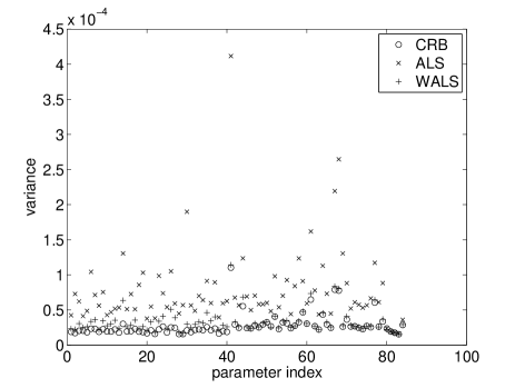
Figure 2: Variance of the parameter vector ${\mbox{\boldmath{$\theta$}}}=[{\mbox{\boldmath{$\gamma$}}}^{T},\phi_{2},\cdots,\phi_{40},$ $\sigma_{2}^{2},\cdots,\sigma_{5}^{2},\sigma_{n}^{2}]^{T}$ estimates obtained in Monte Carlo simulations for the weighted and unweighted versions of the alternating least squares algorithm and compared these results with the CRB.

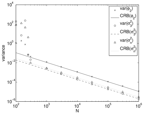
Figure 3: Variances on $\phi_{2}$. $\sigma_{3}^{2}$ and $\sigma_{n}^{2}$ as function of the number of samples $N$, compared to the corresponding CRBs.

Figure 3 shows the variance found on a number of representative parameters as function of the number of samples and compares this with the corresponding CRBs. This plot confirms the conjecture raised in the previous paragraph that the WALS method is asymptotically statistically efficient. Figure 4 shows the bias found in the Monte Carlo simulations and compares this with the statistical error of 1$\sigma$ for a single realization based on the CRB. This result indicates that both methods are unbiased for all parameters.

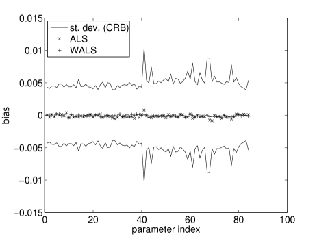
Figure 4: Bias on the estimated parameters (${\mbox{\boldmath{$\theta$}}}=[{\mbox{\boldmath{$\gamma$}}}^{T},\phi_{2},\cdots,\phi_{40},$ $\sigma_{2}^{2},\cdots,\sigma_{q}^{2},\sigma_{n}^{2}]^{T}$) for the weighted and unweighted version of the alternating least squares algorithm in the Monte Carlo simulations. The bias is compared with the standard deviation on the estimates derived from the CRB.

Figure 5 shows the difference of the parameter value at the end of each iteration and its final value obtained from one run of the Monte Carlo simulation for a representative case, i.e. similar results were found for other parameters and other runs. The standard deviation based on the CRB is plotted as reference to facilitate the interpretation of the vertical scale. The results indicate that only one or two iterations are needed to reach the CRB in this scenario. With regard to other scenarios, this result suggests exponential convergence, i.e. each iteration adds about one significant digit to the parameter estimate, and it indicates that the WALS method converges more rapidly than the ALS method. In these simulation the stop criterion was $|{\mbox{\boldmath{$\theta$}}}^{[i-1]\dagger}{\mbox{\boldmath{$\theta$}}}^{[i]}-1|<10^{-10}$.

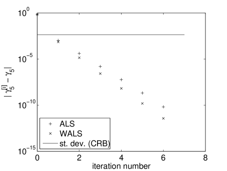
Figure 5: The difference between the value of $\widehat{\gamma}_{5}$ at the end of each iteration and its final value is plotted versus the iteration number for ALS and WALS obtained in one of the Monte Carlo simulation runs. The behavior shown in this plot is representative for the results obtained for other parameters and from other runs. The standard deviation based on the CRB is also shown to demonstrate that one but preferably two iterations are sufficient to obtain a sufficiently accurate result.

In the second simulation the direction independent gains, the apparent source powers and source locations and the receiver noise powers were estimated assuming an array of ideal elements. This corresponds to the third scenario described in section II. The parameter vector to be estimated is thus ${\mbox{\boldmath{$\theta$}}}=[{\mbox{\boldmath{$\gamma$}}}^{T},\phi_{2},\cdots,\phi_{40},\sigma_{2}^{2},\cdots,\sigma_{5}^{2},\sigma_{n}^{2},l_{2},\cdots,l_{5},m_{2},\cdots,m_{5}]^{T}$. Data were generated assuming $\sigma_{n}^{2}=10$ and $N=1000$. This again implies an instantaneous SNR of only 0.1 per array element but in this case the SNR per receiver is only 3.2 for the strongest source after integration. Figure 6 shows the variance on the estimated parameters based on 1000 runs and compares these results with the CRB. In these simulations we only used the xWALS algorithm, since the previous simulations demonstrated that the ALS method gives inferior results compared to the WALS approach. These results show that the variance on the parameter estimates are close to the CRB.

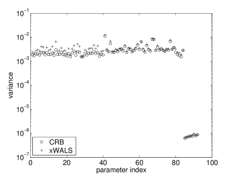
Figure 6: Variance on the parameter vector ${\mbox{\boldmath{$\theta$}}}=[{\mbox{\boldmath{$\gamma$}}}^{T},\phi_{2},\cdots,\phi_{40},$ $\sigma_{2}^{2},\cdots,\sigma_{5}^{2},\sigma_{n}^{2},l_{2},\cdots,l_{5},m_{2}\cdots,m_{5}]^{T}$ estimates obtained in Monte Carlo simulations for the xWALS method, compared with the CRB.

Figure 7 shows the bias on the estimated parameters found in these Monte Carlo simulations. These results indicate that the estimates are unbiased.

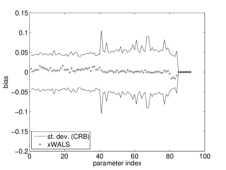
Figure 7: Bias on the estimated parameters (${\mbox{\boldmath{$\theta$}}}=[{\mbox{\boldmath{$\gamma$}}}^{T},\phi_{2},\cdots,\phi_{40},$ $\sigma_{2}^{2},\cdots,\sigma_{5}^{2},\sigma_{n}^{2},l_{2},\cdots,l_{5},m_{2}\cdots,m_{5}]^{T}$) for the xWALS algorithm obtained in Monte Carlo simulations. The results are compared with the standard deviation on the estimated derived from the CRB.

The convergence of a representative parameter is shown in Fig. 8. Again one but preferably two iterations are sufficient to get accurate results. However, in this scenario the stop criterion $|{\mbox{\boldmath{$\theta$}}}^{[i-1]\dagger}{\mbox{\boldmath{$\theta$}}}^{[i]}-1|<10^{-10}$ was not reached and the algorithm stops because the maximum number of iterations. which was set to 15, was reached. This indicates that the algorithm tries to interpret the noise as real signal. In the first iteration first the omnidirectional gains, apparent source powers and noise power are estimated. These values are then used in the WSF to find the source locations. The source locations are then used to update the sky model, leading to an update of $\widehat{\mbox{\boldmath{$\gamma$}}}$, $\widehat{\mbox{\boldmath{$\sigma$}}}$ and $\widehat{\mbox{\boldmath{$\sigma$}}}_{n}$ and the cycle is complete. In the first simulation, the SNR after integration defined as $\sqrt{N}\sigma_{i}^{2}/\sigma_{n}^{2}$ was a factor 10 better than in this simulation in which the SNR per array element per source after integration is only 2.2 to 3.2.

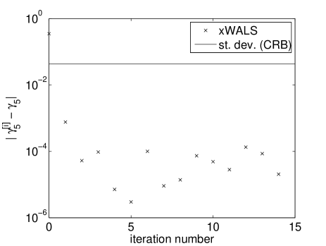
Figure 8: The difference between the value of $\widehat{\gamma}_{5}$ at the end of each iteration and its final value is plotted versus the iteration number for one of the Monte Carlo simulation runs. The behavior shown in this plot is representative for the results obtained for other parameters and from other runs. The standard deviation based on the CRB is also shown to demonstrate that one but preferably two iterations are sufficient to obtain a sufficiently accurate result.

VI Summary and conclusions

In this paper we have developed a weighted alternating least squares (WALS) algorithm to solve for direction independent complex gains, apparent source powers and receiver noise powers simultaneously in a snapshot observation by a sensor array. Our solution for finding the direction independent gains extends and improves the available methods in the literature in the case of multiple calibrator sources and provides robustness to small entries in the array covariance matrix and small gain values (due to e.g. failing elements). Although we have assumed independent sensor noise powers, our gain estimation method is easily applied to cases in which some pairs of elements experience correlated noise. We also found that unbiased estimation of the receiver noise powers requires weighting with the best available array covariance matrix model instead of weighting with the measured array covariance matrix, which is common practice in signal processing.

The statistical performance was compared with an unweighted alternating least squares (ALS) algorithm and the CRB and found to provide a statistically efficient estimate thereby outperforming the ALS method. The computational complexity of ALS and WALS scale with $4\frac{1}{2}p^{3}$ and about $7p^{3}$ respectively assuming that the number of calibrator sources is much smaller than the number of array elements, i.e. the WALS method comes with only a minor increase in computational burden. Simulations indicate that only one or two iterations are sufficient to reach the CRB and that every iteration adds about one significant digit, the WALS method converging slightly faster than the ALS method.

We extended these methods with source location estimation using weighted subspace fitting. Simulations indicate that this extension to the WALS algorithm provides a statistically efficient simultaneous estimate of omnidirectional gains, apparent source powers, source locations and receiver noise powers. Again, one to two iterations proved to be sufficient to reach the CRB. However, the convergence of the parameter is blocked at some level lower than the CRB by the noise in the measurement, at which point the algorithm keeps jumping from one local optimum to another.

VII Acknowledgments

This work has been carried out in close collaboration with the LOFAR-team. This helped to develop our ideas up to the point at which our method could be implemented to calibrate the LOFAR stations. Especially the interaction with Albert-Jan Boonstra and Jaap Bregman at ASTRON on LOFAR station calibration is gratefully acknowledged. The authors would also like to thank the reviewers whose comments helped to improve the original manuscript.

Stefan J. Wijnholds (S’2006) was born in The Netherlands in 1978. He received M.Sc. degrees in Astronomy and Applied Physics (both cum laude) from the University of Groningen in 2003. After his graduation he joined the R&D department of ASTRON, the Netherlands Institute for Radio Astronomy, in Dwingeloo, The Netherlands, where he works with the system design and integration group on the development of the next generation of radio telescopes. Since 2006 he is also with the Delft University of Technology, Delft, The Netherlands, where he is pursuing a Ph.D. degree. His research interests lie in the area of array signal processing, specifically calibration and imaging.

Alle-Jan van der Veen (F’2005) was born in The Netherlands in 1966. He received the Ph.D. degree (cum laude) from TU Delft in 1993. Throughout 1994, he was a postdoctoral scholar at Stanford University. At present, he is a Full Professor in Signal Processing at TU Delft. He is the recipient of a 1994 and a 1997 IEEE Signal Processing Society (SPS) Young Author paper award, and was an Associate Editor for IEEE Tr. Signal Processing (1998–2001), chairman of IEEE SPS Signal Processing for Communications Technical Committee (2002-2004), and Editor-in-Chief of IEEE Signal Processing Letters (2002-2005). He currently is Editor-in-Chief of IEEE Transactions on Signal Processing, and member-at-large of the Board of Governors of IEEE SPS. His research interests are in the general area of system theory applied to signal processing, and in particular algebraic methods for array signal processing, with applications to wireless communications and radio astronomy.

References

- [1] J. D. Bregman, “LOFAR Approaching the Critical Design Review,” in Proceedings of the XXVIIIth General Assembly of the International Union of Radio Science (URSI GA), New Delhi, India, Oct. 23-29 2005.
- [2] C. J. Lonsdale, “The Murchison Widefield Array,” in Proceedings of the XXIXth General Assembly of the Internatio nal Union of Radio Science (URSI GA), Chicago (Ill.), USA, Oct. 7-16, 2008.
- [3] J. B. Peterson, U. L. Pen and X. P. Wu, “The Primeval Structure Telescope: Goals and Status,” in Proceedings of the XXVIIIth General Assembly of the Internatio nal Union of Radio Science (URSI GA), New Delhi, India, Oct. 23-29 2005.
- [4] C. Lonsdale, “Calibration Approaches,” MIT Haystack, Tech. Rep. LFD memo 015, Dec. 8, 2004.
- [5] T. Cornwell and E. B. Fomalont, “Self-Calibration,” in Synthesis Imaging in Radio Astronomy, ser. Astronomical Society of the Pacific Conference Series, R. A. Perley, F. .R. Schwab and A. H. Bridle, Ed. BookCrafters Inc., 1994, vol. 6.
- [6] A. J. Boonstra and A. J. van der Veen, “Gain Calibration Methods for Radio Telescope Arrays,” IEEE Trans. Signal Processing, vol. 51, no. 1, pp. 25–38, Jan. 2003.
- [7] S. J. Wijnholds and A. J. Boonstra, “A Multisource Calibration Method for Phased Array Radio Telescopes,” in Fourth IEEE Workshop on Sensor Array and Multi-channel Processing (SAM), Waltham (MA), 12-14 July 2006.
- [8] S. van der Tol, B. D. Jeffs and A. J. van der Veen, “Self Calibration for the LOFAR Radio Astronomical Array,” IEEE Trans. Signal Porcessing, vol. 55, no. 9, pp. 4497–4510, Sept. 2007.
- [9] B. P. Flanagan and K. L. Bell, “Array Self-Calibration with Large Sensor Position Errors,” in IEEE Internatioal Conference on Acoustics, Speech and Signal Processing (ICASSP), 1999.
- [10] D. Astély, A. L. Swindlehurst and B. Ottersten, “Spatial Signature Estimation for Uniform Linear Arrays with Unknown Receiver Gains and Phases,” IEEE Trans. Signal Processing, vol. 47, no. 8, pp. 2128–2138, Aug. 1999.
- [11] M. Pesavento, A. B. Gershman and K. M. Wong, “Direction Finding in Partly Calibrated Sensor Arrays Composed of Multiple Subarrays,” IEEE Trans. Signal Processing, vol. 50, no. 9, pp. 2103–2115, Sept. 2002.
- [12] C. M. S. See and A. B. Gershman, “Direction of Arrival Estimation in Partly Calibrated Subarray-Based Sensor Arrays,” IEEE Trans. Signal Processing, vol. 52, no. 2, pp. 329–338, Feb. 2004.
- [13] A. J. Weiss and B. Friedlander, “Array Shape Calibration Using Sources in Unknown Locations - A Maximum Likelihood Approach,” IEEE Trans. Acoustics, Speech and Signal Processing, vol. 37, no. 12, Dec. 1989.
- [14] C. M. S. See, “Method for Array Calibration in High-Resolution Sensor Array Processing,” IEE Proc. Radar, Sonar and Navig., vol. 142, no. 3, June 1995.
- [15] J. Pierre and M. Kaveh, “Experimental Performance of Calibration and Direction Finding Algorithms,” in IEEE International Conference on Acoustics, Speech and Signal Processing (ICASSP), vol. 2, May 1991, pp. 1365–1368.
- [16] B. C. Ng and C. M. S. See, “Sensor Array Calibration Using a Maximum Likelihood Approach,” IEEE Trans. Antennas and Propagation, vol. 44, no. 6, June 1996.
- [17] H. Li, P. Stoica and J. Li, “Computationally Efficient Maximum Likelihood Estimation of Structured Covariance Matrices,” IEEE Trans. Signal Processing, vol. 47, no. 5, pp. 1314–1323, May 1999.
- [18] A. J. Weiss and B. Friedlander, “’Almost Blind’ Signal Estimation Using Second-Order Moments,” IEE Proc. Radar, Sonar and Navig., vol. 142, no. 5, Oct. 1995.
- [19] M. Zatman, “How Narrow is Narrowband,” IEE Proc. Radar, Sonar and Navig., vol. 145, no. 2, pp. 85–91, Apr. 1998.
- [20] D. R. Fuhrmann, “Estimation of Sensor Gain and Phase,” IEEE Trans. Signal Processing, vol. 42, no. 1, pp. 77–87, Jan. 1994.
- [21] S. J. Wijnholds and A. J. van der Veen, “Effects of Parametric Constraints on the CRLB in Gain and Phase Estimation Problems,” IEEE Signal Processing Letters, vol. 13, no. 10, pp. 620–623, Oct. 2006.
- [22] S. Kay, Fundamentals of Statistical Signal Processing: Estimation Theory. Englewood Cliffs, New Jersey: Prentice Hall, 1993, vol. 1.
- [23] B. Ottersten, P. Stoica and R. Roy, “Covariance Matching Estimation Techniques for Array Signal Processing Applications,” Digital Signal Processing, A Review Journal, vol. 8, pp. 185–210, July 1998.
- [24] T. J. Pearson and A. C. S. Readhead, “Image Formation by Self-Calibration in Radio Astronomy,” Ann. Rev. Astron. Astrophys., vol. 22, pp. 97–130, 1984.
- [25] S. van der Tol and S. J. Wijnholds, “CRB Analysis of the Impact of Unknown Receiver Noise on Phased Array Calibration,” in Fourth IEEE Workshop on Sensor Array and Multi-channel Processing (SAM), Waltham (MA), 12-14 July 2006.
- [26] R. O. Schmidt, “Multiple Emitter Location and Signal Parameter Estimation,” IEEE Trams. Antennas and Propagation, vol. AP-34, no. 3, Mar. 1986.
- [27] M. Viberg and B. Ottersten, “Sensor Array Processing Based on Subspace Fitting,” IEEE Trans. Signal Processing, vol. 39, no. 5, pp. 1110–1121, May 1991.
- [28] M. Viberg, B. Ottersten and T. Kailath, “Detection and Estimation in Sensor Arrays Using Weighted Subspace Fitting,” IEEE Trans. Signal Processing, vol. 39, no. 11, pp. 2436–2448, Nov. 1991.
- [29] A. Quinlan, J.-P. Barbot and P. Larzabal, “Automatic Determination of the Number of Targets Present When Using the Time Reversal Operator,” Journal of the Acoustic Society of America, vol. 119, no. 4, pp. 2220–2225, Apr. 2006.
- [30] A. Quinlan, J. P. Barbot, P. Larzabal and M. Haardt, “Model Order Selection for Short Data: An Exponential Fitting Test (EFT),” EURASIP Journal on Advances in Signal Processing, 2007.
- [31] M. Wax and T. Kailath, “Detection of Signals by Information Theoretic Criteria,” IEEE Trans. Acoustics, Speech and Signal Processing, vol. ASSP-33, no. 2, pp. 387–392, Apr. 1985.
- [32] Divide-and-conquer eigenvalue algorithm. [Online]. Available: http://en.wikipedia.org/wiki/Divide-and-conquer_eigenvalue_algorithm
- [33] T. K. Moon and W. C. Stirling, Mathematical Methods and Algorithms for Signal Processing. Prentice Hall, 2000.