Odd spin-triplet superconductivity in a multilayered superconductor-ferromagnet Josephson junction.

Abstract

We study the dc Josephson effect in a diffusive multilayered SF’FF’S structure, where S is a superconductor and F,F’ are different ferromagnets. We assume that the exchange energies in the F’ and F layers are different ($h$ and $H$, respectively) and the middle F layer consists of two layers with parallel or antiparallel magnetization vectors $M$. The $M$ vectors in the left and right F’ layers are generally not collinear to those in the F layer. In the limit of a weak proximity effect we use a linearized Usadel equation. Solving this equation, we calculate the Josephson critical current for arbitrary temperatures, arbitrary thicknesses of the F’ and F layers ($L_{h}$ and $L_{H}$) in the case of parallel and antiparallel $M$ orientations in the F layer. The part of the critical current $I_{cSR}$ formed by the short-range (SRC) singlet and $S=0$ triplet condensate components decays on a short length $\xi_{H}=\sqrt{D/H}$, whereas the part $I_{cLR}$ due to the long-range triplet $|S|=1$ component (LRTC) decreases with increasing $L_{H}$ on the length $\xi_{N}=\sqrt{D/\pi T}$. Our results are in a qualitative agreement with the experiment Birge .

I Introduction

According to the Bardeen, Cooper and Schrieffer BCS theory of superconductivity in conventional metals and their alloys the superconducting condensate consists of singlet Cooper pairs. These pairs can be described by a wave function $f$ which is in the absence of the condensate flow symmetric in the momentum space ($s$-wave singlet pairing). In terms of the creation and annihilation operators $\psi^{+},\psi,$ this function can be represented in the form of a thermodynamic average $f_{sng}(t-t^{\prime})\sim\langle\psi_{\uparrow}(t)\psi_{\downarrow}(t^{\prime})-\psi_{\downarrow}(t^{\prime})\psi_{\uparrow}(t)\rangle.$ At equal times ($t=t^{\prime}$) this function determines the order parameter $\Delta:$ $\Delta=\lambda\langle\psi_{\uparrow}(t)\psi_{\downarrow}(t)\rangle=-\lambda\langle\psi_{\downarrow}(t)\psi_{\uparrow}(t)\rangle$, where $\lambda$ is the coupling constant of an attractive interaction.The spin-independent scattering by ordinary impurities does not affect this type of superconductivity (Anderson-theorem) Schrieffer .

In the last two decades other types of superconductivity have been discovered. The most important example is high $T_{c}$ superconductivity discovered by Bednorz and Müller BednorzMuller in cuprates.

As a result of intensive study of these superconductors, it was demonstrated that, although the Cooper pairs in this case are also singlet, their wave function essentially depends on the momentum $p$ and changes sign with varying momentum direction in $CuO$ planes. In the simplest version, the dependence of the order parameter $\Delta$ on $p$ has the form: $\Delta(\mathbf{p})=\Delta_{0}(\cos^{2}(p_{x}a_{x})-\cos^{2}(p_{y}a_{y}))$ ($d$-wave singlet pairing). Such a dependence $\Delta(\mathbf{p})$ allows one to construct the so called $\pi-$Josephson junction consisting of single crystals of high T_c superconductors with an appropriate orientation of these crystals with respect to each other Harlingen ; Kirtley . The ground state of this junction corresponds to the phase difference equal to $\pi$.

Another type of superconductivity (triplet) has been discovered in strontium ruthinate $Sr_{2}RuCu_{4}$ Maeno ; Eremin and in heavy fermion intermetallic compounds Mineev . In contrast to the singlet superconductivity, the wave function of the Cooper pairs $f_{\uparrow\uparrow}(\mathbf{p+p}^{\prime}\mathbf{,}t-t^{\prime})\sim\langle\psi_{\uparrow}(\mathbf{p,}t)\psi_{\uparrow}(\mathbf{p}^{\prime}\mathbf{,}t^{\prime})\rangle$ is an odd function of momentum $\mathbf{p}$, so that for equal times $t=t^{\prime}$ the function $f_{\uparrow\uparrow}(\mathbf{p,}0)$ and the order parameter $\Delta(\mathbf{p})$ do not equal to zero ($p$-wave triplet pairing). Only for some directions of the momentum $\mathbf{p}$ the order parameter turns to zero. This means that, in agreement with the Pauli principle, the pair wave function changes sign under permutation of spins and momenta. The momentum dependence of the condensate function makes the singlet $d$-wave and triplet $p$-wave superconductivity sensitive to scattering even by potential (not acting on spin) impurities.

An unusual mechanism of superfluidity was proposed by Berezinsky Berez . Having in mind liquid $He^{3}$, he considered a retarded interaction between atoms and assumed that the order parameter $\Delta(\omega)$ and the wave functions $f_{\uparrow\uparrow}(\mathbf{p,}\omega)$ or $f_{\downarrow\downarrow}(\mathbf{p,}\omega)$ in the Matsubara representation were even functions of momentum but odd function of the Matsubara frequency $\omega$. However, experiments on superfluid $He^{3}$ revealed that the $p$-wave triplet type of the superfluidity is realized in $He^{3}$ rather than the one proposed by Berezinsky Leggett ; Wolfle . Some possibilities to realize the exotic Berezinsky-type mechanism of superconductivity in various systems in context of the pairing mechanism in high $T_{c}$ superconductors were considered in Refs.Kirkpatrick ; Coleman ; Abrahams .

This exotic type of superconductivity (or superfluidity) was regarded for quite a long time as a hypothetical one. Only recently it has been realized BVE01 that the odd triplet superconductivity might exist in a simple  SF bilayer system consisting of a conventional $s$-wave singlet BCS-type superconductor S and a ferromagnetic layer F with a nonhomogeneous magnetization $M.$

To that moment it had already been well known that in an SF system with a homogeneous magnetization $M$ the Cooper pairs penetrated the ferromagnet over a short length $\xi_{F}=\sqrt{D/E_{ex}}$ (in the diffusive limit), where $D=vl/3$ is the diffusion coefficient, $l=v\tau$ is the mean free path, and $E_{ex}$ is the exchange energy in the ferromagnet (we set the Planck constant $\hbar$ equal to $1$). Since the exchange energy usually is much larger than the critical temperature of the superconductor $T_{c}$, the length $\xi_{F}$ is much shorter than the length of the condensate penetration into a normal metal in an SN bilayer: $\xi_{N}=\sqrt{D/\pi T}$ deGennes ; GolubovRMP ; BuzdinRMP ; BVErmp .

The Cooper pairs penetrating the ferromagnet with an uniform magnetization consist of electrons with opposite spins. Their wave function is however the sum of a singlet and triplet component with zero total spin projection on the $z$-axis ($S=0$). The exchange field mixes these components and the triplet component with $S=0$ is unavoidable in the ferromagnet. The sum of these two components can be considered as a short-range component (SRC).

The part corresponding the triplet $S=0$ component has the form $f_{tr\uparrow\downarrow}(t-t^{\prime})\sim\langle\psi_{\uparrow}(t)\psi_{\downarrow}(t^{\prime})+\psi_{\downarrow}(t^{\prime})\psi_{\uparrow}(t)\rangle$. At equal times $t=t^{\prime}$ this function equals zero in agreement with the Pauli principle. Therefore the function $f_{tr\uparrow\downarrow}(t-t^{\prime})$ is an odd function of the time difference $(t-t^{\prime})$ or $\omega$ in the Matsubara representation. The order parameter in the superconductor S is related only to the singlet function $f_{sng}(\omega)$ which is an even function of $\omega.$ The superconducting order parameter in F is zero if the coupling constant $\lambda_{F}$ in the Cooper channel equals zero.

The situation changes if the magnetization orientation in the vicinity of the SF interface is not fixed. This case was analyzed in Ref. BVE01 , where an SF bilayer with a domain wall located at the SF interface was considered. It was shown that in such a system not only the singlet and triplet $S=0$ components but also the odd triplet component with $S=\pm 1$ arises in the ferromagnet. The latter component penetrates the superconductor over a large distance that does not depend on the exchange field and is of the order $\xi_{N}$ provided the spin-dependent scattering is not too strong.

This odd triplet component can be considered as the long-range triplet component (LRTC). As the LRTC is symmetric in the momentum space, the scattering by potential impurities does not affect this component.

In subsequent theoretical papers various types of SF structures where the LRTC may arise were studied (see review articles BVErmp ; BuzdinRMP ; EschrigRev and references therein). In Ref. BVE01 the creation of the LRTC is predicted in a diffusive SF structure with a Bloch-type domain wall (DW). The width of the DW, $w,$ was assumed to be larger than the mean free path $l:$ $l\ll$ $\{w,\xi_{F}\}.$

A more general case of the DW with a width, arbitrary with respect to the mean free path, in a SF structure with an arbitrary impurity concentration was studied in Ref. VE08 . The LRTC in diffusive SF structures with a Neel-type DWs has been analyzed in Ref. Fominov05 . The case of a half-metallic ferromagnet in SF or SFS structures was investigated in Refs. Eschrig03 ; AsanoBC ; Zaikin08 . Braude and Nazarov Braude studied the LRTC in SF structures with a highly transparent SF interfaces so that the amplitude of the condensate functions induced in the ferromagnet was not small (strong proximity effect). Ballistic SF structures with a nonhomogeneous magnetization, where the LRTC could be created, were studied in Refs. Radovic ; Beenakker ; Valls ; AsanoBC . The papers VAE06 ; Champel08 ; Annett ; SudboSp were devoted to the study of the LRTC in spiral ferromagnets attached to superconductors.

In several papers Eschrig03 ; AsanoBC ; Sudbo ; ZaikinBC ; Belzig+Naz the LRTC was investigated in SF structures with the so-called spin-active interfaces. In the approach used in these papers, the properties of the SF interface are characterized by a scattering matrix with elements considered as phenomenological parameters. In this approach one does not need knowing the detailed structure of the SF interface and can proceed calculating physical quantities using these parameters. We will see that even in the framework of the quasiclassical theory one can obtain effective boundary conditions for the LRTC provided the width of the DW $w$ attached at the SF interface is thin enough (such an approach was used in Ref. VE08 ). From the physical point of view the region with a narrow DW can be regarded as a spin-active SF interface. If the width $w$ is comparable with the Fermi wave length, one has to go beyond the quasiclassical theory and derive the boundary conditions from the first principles (see Millis as well as EschrigBC09 ; Belzig+Naz and references therein).

By now, several papers presenting a quite convincing experimental evidence in favor of the existence of the LRTC have been published Petrashov ; Klapwijk ; Birge ; Aarts10 . In Ref. Petrashov the conductance of a spiral ferromagnet ($Ho$) attached to two superconductors was measured. It was concluded that the conductance variation below the superconducting critical temperature $T_{c}$ is too large to be explained in terms of the singlet component. Keizer et al. Klapwijk observed the Josephson effect in an SFS junction with a half-metallic ferromagnet $CrO_{2}$. The thickness of the F layer was much larger (up to $\sim$1 mkm) than the penetration depth of the short range condensate components. Moreover, in the metal where free electrons with only one spin direction are allowed, no pairs with opposite spins are possible. Therefore, only triplet $|S|=1$ component can survive in this ferromagnet Eschrig03 . However, there is no controllable parameter in this system that would allow one to change the amplitude of the LRTC. A similar long-range Josephson effect in a SFS junction with $CrO_{2}$ as a ferromagnetic layer was observed by Anwar et al. in a recent work Aarts10 .

Recently the dc long-range Josepshon effect has been observed in a more complicated SFS structure with a controllable parameter Birge . In the experimental setup of this work, F was not a single ferromagnetic layer but a multilayered structure of the NF’NFNF’N type, where N is a nonmagnetic metal, F’ is a weak ferromagnet ($PdNi$ or $CuNi$) and F is a strong ferromagnet ($Co$). The middle F layer was in its turn a trilayer structure consisting of two F layers with antiparallel orientation of magnetization $M$ and of a thin layer ($Ru$) that provides RKKY coupling between the F layers.

The authors of Ref. Birge measured the Josephson critical current $I_{c}$ for different thicknesses $L$ of the F’ and F layers (we denote the thicknesses of the F’ and F layers as $L_{h}$ and $L_{H}$ layers respectively). It was demonstrated that in the absence of the F’ layers ($L_{h}=0$) the critical current $I_{c}$ was negligible if the width of the F layer $L_{H}$ essentially exceeded the small length $\xi_{H}=\sqrt{D/H}$, where $H$ is the exchange energy in the F layer. This is what one expects for the conventional superconductivity. However, adding the F’ layers resulted in an increase of the critical current $I_{c}$ by several orders. The dependence of $I_{c}(L_{h})$ is non-monotonous: the critical current is small at small and large $L_{h}$ reaching a maximum at $L_{h}\sim\xi_{h}$.

The authors of Ref.Birge suggested an explanation of these results in terms of the LRTC. Note that the mean free path $l$ in the structure studied in Ref.Birge is rather short (the diffusive limit in the F’ layers and an intermediate case in the F layer).

Theoretically the dc Josephson effect in multilayered SFS junctions with a non-collinear magnetization orientation has been studied in several works. In Refs. Radovic ; Barash the Josephson current in ballistic SFS junctions was calculated. The diffusive SFF’S junctions were considered in Refs. Ivanov ; SudboJJ . However the long-range Josephson effect in the junctions with two F layers is not possible; the Josephson critical current $I_{c}$ is not exponentially small only if the total thickness of the ferromagnetic layer, $L_{F}+L_{F^{\prime}}$, is comparable with the short length $\xi_{F}$: $I_{c}\sim\exp(-(L_{F}+L_{F^{\prime}})/\xi_{F}).$

The diffusive Josephson junctions with three ferromagnetic layers and non-collinear $M$ orientation, where the long-range Josephson coupling may exist, have been analyzed in Refs. BVE03 ; BuzdinHouzet . The authors of Ref. BVE03 considered the F’SFSF’structure with different magnetization $M$ orientations in the F and F’ layers. In Ref. BuzdinHouzet a somewhat different, but more suitable for experimental realization, SF’FF’S structure with different $M$ directions in the F and F’ parts was analyzed. In both papers the exchange energy in the F and F’ was assumed to be equal.

The amplitude of the LRTC, $f_{1},$ and the Josephson critical current due to this component $I_{cLR}$ are calculated in both works. Although the structures studied in Refs. BVE03 ; BuzdinHouzet are different, the results obtained are similar. The final formula for the critical current can be written in both the cases as

$$I_{cLR}=F(L_{h})\sin\alpha_{l}\sin\alpha_{r}$$ (1)

In Eq. (1), $\alpha_{l,r}$ are angles between the $z$-axis and the magnetization vectors in the left (right) F’ layers, while the magnetization $M$ in the F layer is assumed to be parallel to the $z$-axis. The function $F(L_{h})$ is a non-monotonic function with a maximum at $L_{h}\sim\xi_{h}$. This function vanishes at small and large thickness $L_{h}$ of the F’ layers (see Eq. (12) in Ref. BVE03 and Fig. 2 in Ref. BuzdinHouzet ).

Qualitatively, this prediction agrees with the observations in Ref. Birge . However, experimental parameters presented in this publication are well defined and this makes a more detailed comparison of the theoretical predictions for LTRC with the experimental results quite interesting.

In this paper we analyze an SF’FF’S structure which, being formally similar to that considered by Houzet and Buzdin BuzdinHouzet , is in many respects different and closer to the structure studied experimentally.

First, unlike Ref.BuzdinHouzet , we assume that the exchange energies in the F’ and F layers ($h$ an $H$ respectively) are different.

Secondly, we assume that the SF’ interface is not perfect and the proximity effect is weak. This assumption allows us to linearize the Usadel equation and to calculate the critical Josephson current $I_{c}$ at any temperatures $T$ (in Ref. BuzdinHouzet only the case of temperatures close to $T_{c}$ was considered).

Thirdly, we also analyze the case when the F layer consists of two domains with parallel and antiparallel orientations of magnetization.

At last, we derive a formula for the current $I_{c}$ for arbitrary thicknesses, $L_{h,H}$, of the F’ and F layers (in Ref. BuzdinHouzet a formula for $I_{c}$ is presented only in the limit $L_{h}/\xi_{h}\ll 1$).

The paper is organized as follows. In Section II we formulate the problem and write down necessary equations. In Section III we analyze the case of thin F’ layers ($L_{h}/\xi_{h}\ll 1$). We calculate the amplitudes of the short range singlet and triplet $S=0$ components as well as the LRTC. In Section IV the case of arbitrary lengths $L_{h,H}$ will be considered under assumption that the angles $\alpha_{l,r}$ are small. Using the formulas obtained for the amplitudes of different components, we calculate in Section V the critical current $I_{c}$ in the limiting cases: a) for parallel and antiparallel $M$ orientations in the F layer and for arbitrary angles $\alpha_{l,r}$ assuming that the thickness $L_{h}$ is small, b) for arbitrary $L_{h,H}$ under assumption of small $\alpha_{l,r}$. The results obtained are discussed in Section VI.

II Model and Basic Equations

We consider a multi-layer S/F Josephson junction shown schematically in Fig.1. It consists of two superconductors, S, and three ferromagnetic layers F, F’${}_{\text{r,l}}$. The middle F layer may consist of two domains or layers with parallel or antiparallel orientations of the magnetization $M$. A similar Josephson junction has been studied experimentally in a recent work Birge .

The presence of normal N layers in the experimental S/NF${}_{\text{l}}$NFNF${}_{\text{r}}$N/S structures cannot change qualitatively the results for the S/F’${}_{\text{l}}$FF’${}_{\text{r}}/$S structure obtained here because the scattering in the N layers does not depend on spin (if a weak spin-orbit scattering can be neglected). Therefore, all the superconducting components, singlet and triplet, decay in the N layers in a similar way over a large distance of the order $\xi_{N}$. The exchange fields acting on electron spins are $h$ in the F^′ layers and $H$ in the middle F layer. The magnetization vector $\mathbf{M}$ in F is supposed to align along the z-axis and it has the components $M(0,\sin\alpha_{l,r},\cos\alpha_{l,r})$ in the F’${}_{\text{l,r}}$ layers. The magnetization in the F layer is oriented along the $z$-axis but may have parallel or antiparallel orientations in the regions ($-L_{H}<x<0$) and ($0<x<L_{H}$).

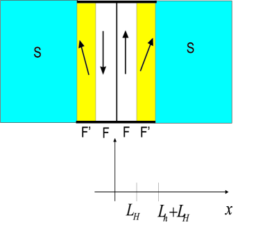
Figure 1: (color online) Josephson structure under consideration. The F’(F) layers are weak (strong) ferromagnets. The middle F layer consists of two layers with parallel or antiparallel (shown in figure) magnetization orientation. The arrows show the directions of the magnetization in F’ and F layers.

For explicit calculations we use the quasiclassical Green’s function technique, which is the most efficient tool for studying SF structures (see reviews LOrev ; KopninRev ; Rammer ; BelzigRev ; GolubovRMP ; BuzdinRMP ; BVErmp ), and assume that all the ferromagnetic layers are in the diffusive regime, so that the Usadel equation can be used. The amplitude of the condensate wave function in the ferromagnetic layers is assumed to be small (weak proximity effect) and therefore the Usadel equation can be linearized. The smallness of the condensate wave function is either due to a mismatch of the Fermi velocities in S and F or due to the presence of a tunnel barrier at the S/F interfaces.

The anomalous (Gor’kov) quasiclassical Green’s function in the considered case of a spin-dependent interaction is a $4\times 4$ matrix $\check{f}$. We are interested in the dc Josephson current $I_{c},$ i.e. in a thermodynamical quantity. Therefore we can use the Matsubara representation for the matrix $\check{f}$  and consider $\check{f}$ as a function of the Matsubara frequency $\omega=\pi T(2n+1)$ and coordinate $x$ normal to interfaces: $\check{f}=\check{f}(\omega,x)$. The linearized Usadel equation for $\check{f}$ has the form (see BVErmp , Eq.(3.15))

$$\partial^{2}\check{f}/\partial x^{2}-\kappa_{\omega}^{2}\check{f}\;-i(\kappa_{F}^{2}/2)\cos\alpha(x)$$

$$\times\{\tan\alpha(x)\hat{\tau}_{3}\mathbf{\otimes}[\hat{\sigma}_{2},\check{f}]+[\hat{\sigma}_{3},\check{f}]_{+}\}=0$$ (2)

where $\kappa_{\omega}^{2}=2|\omega|/D$, $\kappa_{F}^{2}=2\mathit{sgn}\omega\cdot h/D$ in the F’${}_{\text{l,r}}$ layers and $\kappa_{F}^{2}=2\mathit{sgn}\omega\cdot H/D$ in the F layer, the Pauli matrices $\hat{\tau}_{i}\mathbf{,}\hat{\sigma}_{i}$ operate in the particle-hole and spin space respectively. The angle $\alpha$ is equal to $\alpha_{l,r}$ in the F’${}_{\text{l,r}}$ layers and to zero in the F layer in the case of the parallel orientation of the magnetization $M$ in the domains. In the case of the antiparallel orientation $\alpha(x)=\pi$ in the interval ($-L_{H}<x<0$) and $\alpha(x)=0$ in the interval ($0<x<L_{H}$). The diffusion coefficient $D$ is assumed to be the same in all the ferromagnetic layers.

The matrix $\check{f}$ can be represented for the system under consideration in a form of an expansion in the spin matrices $\hat{\sigma}_{i}$ as

$$\check{f}=\hat{f}_{0}\mathbf{\otimes}\hat{\sigma}_{0}+\hat{f}_{1}\mathbf{\otimes}\hat{\sigma}_{1}+\hat{f}_{3}\mathbf{\otimes}\hat{\sigma}_{3}$$ (3)

The matrices $\hat{\sigma}_{0}$ and $\hat{\sigma}_{1,3}$ are the unit matrix and the $\hat{\sigma}_{x,z}$ Pauli matrices, respectively. The $\hat{f}_{0,1,3}$ matrices are matrices in the particle-hole space. The first term is the short range triplet component with the zero projection of the total spin on the z-axis, the second term is the LRTC with the non-zero projection of the total spin, and the third term is the singlet component of the condensate Green’s function (see BVE03 ; BVErmp ).

Eq. (2) should be complemented by boundary conditions. We consider the simplest model of the S/F heterostructures assuming that the interfaces have no effect on spins (spin-passive interface). These boundary conditions have the form ZaitsevBC ; KL

$$\partial\check{f}/\partial x|_{x=\pm L}=\pm\gamma_{B}\check{f}_{S}|_{x=\pm L},$$ (4)

where $\gamma_{B}=1/(R_{B}\sigma),R_{B}$ is the S/F interface resistance per unit area, $\sigma$ is the conductivity of the ferromagnet. The matrix $\check{f}_{S}$ is the Gor’kov’s quasiclassical Green’s function in the left and right superconductors. It has the form

$$\check{f}_{S}|_{x=\pm L}=f_{S}\hat{\sigma}_{3}\mathbf{\otimes}(\hat{\tau}_{2}\cos\varphi\pm\hat{\tau}_{1}\sin\varphi),$$ (5)

where $f_{S}=\Delta/\sqrt{\omega^{2}+\Delta^{2}},$ $\pm\varphi$ is the phase in the right (left) superconductor, so that the phase difference is $2\varphi$.

If there is a spin-dependent interaction in a thin layer at the interface (exchange field, spin-dependent scattering etc), the boundary condition acquires a more complicated form. In particular, the coefficient $\gamma_{B}$ becomes a matrix with matrix elements containing very often unknown phenomenological parameters. Such interfaces are called spin-active interfaces. In many papers the LRTC is studied in SF systems with spin-active interfaces Eschrig03 ; AsanoBC ; Sudbo ; Zaikin08 ; Belzig+Naz .

The F/F’${}_{\text{l,r}}$ interfaces are assumed to be ideal and therefore the function $\check{f}(x)$ and its derivative $\partial\check{f}/\partial x$ must be continuous at these interfaces. Solving the linear equation (2) with the boundary conditions (4) one can calculate the dc Josephson current using the formula BuzdinRMP ; BVErmp

$$j_{J}=(\sigma/8)2\pi T\sum_{\omega\geq 0}Tr\{\hat{\sigma}_{0}\mathbf{\otimes}\hat{\tau}_{3}\check{f}\partial\check{f}/\partial x\},$$ (6)

This problem can be solved in a general case of an arbitrary thicknesses of the F and F’ layers ($L_{H}$ and $L_{h}$) and angles $\alpha_{l,r}$.

However, the general results are too cumbersome. In order to present analytical formulas in a more or less compact form, we consider two limiting cases: a) thin F’${}_{\text{l,r}}$ layers ($L_{h}\ll\xi_{h},\xi_{N}$) and arbitrary angles $\alpha_{r,l}$ , b) arbitrary thicknesses $L_{H},L_{h}$, but small angles $\alpha_{r,l}$ ($\alpha\ll 1$). In the next section we consider the case a).

III Thin F^′ layers

In this section we assume that the F’${}_{\text{l,r}}$ layers (or $h$-layers) are very thin so that the inequality $|\kappa_{h}|L_{h}\ll 1$ is satisfied, where $\kappa_{h}^{2}=2\mathit{sgn}\omega(h/D)$ (usually $\kappa_{h}\gg\kappa_{N}=\sqrt{\pi T/D}$ and therefore the condition $\kappa_{N}L_{h}\ll 1$ is also fulfilled). In the zero order approximation in the parameter $\kappa_{h}L_{h},$ the exchange field in the entire ferromagnetic region except the thin F’${}_{\text{l,r}}$ layers is homogeneous and equal to $H$. Thus, only the $\hat{f}_{0,3}$ components in the expansion (3) that describe the short-range components (SRC) differ from zero.

The matrix $\check{f}$ satisfies the equation

$$\partial^{2}\check{f}/\partial x^{2}-\kappa_{\omega}^{2}\check{f}\;-i\kappa_{H}^{2}\cos\alpha(x)\hat{\sigma}_{3}\mathbf{\otimes}\check{f}=0,$$ (7)

where $\kappa_{H}^{2}=2\mathit{sgn}\omega(H/D)$.

The angle $\alpha(x)=0$ in the case of parallel orientation of the vector $\mathbf{M,}$ and $\alpha(x)=0$ at $x>0$, $\alpha(x)=\pi$ at $x<0$ in the case of antiparallel orientation. We rewrite Eq. (7) for the diagonal in spin space components $\hat{f}_{\pm}=\hat{f}_{0}\pm\hat{f}_{3}$ as

$$\partial^{2}\hat{f}_{\pm}/\partial x^{2}-\kappa_{\pm}^{2}\hat{f}_{\pm} = 0,\text{ \ }x>0,$$ (8)

$$\partial^{2}\hat{f}_{\pm}/\partial x^{2}-\hat{\bar{\kappa}}_{\pm}^{2}\hat{f}_{\pm} = 0,\text{ \ }x<0,$$ (9)

where $\kappa_{\pm}^{2}=\kappa_{\omega}^{2}\pm i\kappa_{H}^{2},$ $\hat{\bar{\kappa}}_{\pm}^{2}=\kappa_{\pm}^{2}$ in the case of the parallel $M$ orientation in both domains ($x>0$ and $x<0$) and $\hat{\bar{\kappa}}_{H}^{2}=\kappa_{\omega}^{2}\mp i\kappa_{H}^{2}$ if the magnetization vector at $x<0$ changes sign with respect to its direction at $x>0$. The boundary conditions for matrices $\hat{f}_{\pm}$ follow from Eq. (4)

$$\partial\hat{f}_{\pm}/\partial x = \pm\gamma_{B}f_{S}(\hat{\tau}_{2}\cos\varphi+\hat{\tau}_{1}\sin\varphi),\text{ }$$

$$\text{\ }x = L_{H},$$ (10)

$$\partial\hat{f}_{\pm}/\partial x = \mp\gamma_{B}f_{S}(\hat{\tau}_{2}\cos\varphi-\hat{\tau}_{1}\sin\varphi),\text{ }$$

$$\text{\ }x = -L_{H};$$ (11)

The solution of Eqs.(8-9) can be sought in the form

$$\hat{f}_{\pm}(x) = \hat{A}_{\pm}\cosh(\kappa_{\pm}x)\cos\varphi+\hat{B}_{\pm}\sinh(\kappa_{\pm}x)\sin\varphi,\text{ }$$

$$\text{\ }x > 0,$$ (12)

$$\hat{f}_{\pm}(x) = \hat{\bar{A}}_{\pm}\cosh(\bar{\kappa}_{\pm}x)\cos\varphi+\hat{\bar{B}}_{\pm}\sinh(\bar{\kappa}_{\pm}x)\sin\varphi,\text{ }$$

$$\text{\ }x < 0,$$ (13)

The relations between coefficients $\hat{A},\hat{\bar{A}}$ and $\hat{B},\hat{\bar{B}}$ should be found from the continuity of the matrices $\hat{f}_{\pm}(x)$ and their derivatives $\partial\hat{f}_{\pm}/\partial x$ at $x=0$. This gives: $\hat{A}=\hat{\bar{A}},$ $\kappa_{H}\hat{B}=\bar{\kappa}_{H}\hat{\bar{B}}.$ Using the boundary conditions (10,11), we find the coefficients $\hat{A}_{\pm},\hat{B}_{\pm}$

$$\hat{A}_{\pm} = \pm\frac{\gamma_{B}}{\mathcal{D}_{\pm}}[\hat{f}_{S}(L_{H})\cosh\bar{\theta}_{\pm}+\hat{f}_{S}(-L_{H})\cosh\theta_{\pm}],$$

$$\hat{B}_{\pm} = \pm\frac{\gamma_{B}}{\mathcal{D}_{\pm}}[\hat{f}_{S}(L_{H})\frac{\bar{\kappa}_{\pm}}{\kappa_{\pm}}\sinh\bar{\theta}_{\pm}-\hat{f}_{S}(-L_{H})\sinh\theta_{\pm}],$$

where $\mathcal{D}_{\pm}=\kappa_{\pm}\sinh\theta_{\pm}\cosh\bar{\theta}_{\pm}+\bar{\kappa}_{\pm}\sinh\bar{\theta}_{\pm}\cosh\theta_{\pm},$ $\theta_{\pm}=\kappa_{\pm}L_{H}$ and $\bar{\theta}_{\pm}=\bar{\kappa}_{\pm}L_{H}.$

In the case of parallel (P) and antiparallel (AP) orientations of the magnetization in the F layer we obtain the function $\mathcal{D}_{\pm}$

$$\mathcal{D}_{\pm P} = 2\kappa_{\pm}\sinh\theta_{\pm}\cosh\theta_{\pm}\text{ },$$

$$\text{ }\mathcal{D}_{+AP} = \mathcal{D}_{-AP}=2Re(\kappa_{+}\sinh\theta_{+}\cosh\theta_{-}).$$

One can see from Eqs. (12-LABEL:Bpm) that the SRC decays exponentially away from the SF interfaces over the short length $\xi_{H}.$ Indeed, at $|L_{H}-x|\gg\xi_{H}$ we obtain from Eqs. (12-LABEL:Bpm) that $\hat{f}_{\pm}(x)\sim(\gamma_{B}/\kappa_{\pm})f_{S}(\hat{\tau}_{2}\cos\varphi+\hat{\tau}_{1}\sin\varphi)\exp(-(L_{H}-x)/\xi_{H}).$

Let us now find the LRTC. First, we obtain the effective boundary conditions for this component. Assuming that $L_{h}\ll\xi_{h}$, we can integrate Eq.(2) over the thickness of the F’-layers and come to effective boundary conditions for the triplet component

$$\partial\hat{F}_{1}/\partial x|_{x=\pm L_{H}}=\pm\gamma_{1}\hat{f}_{3}(\pm L_{H})\sin\alpha_{r,l},\text{ }$$ (16)

where $\gamma_{1}\equiv\kappa_{h}^{2}L_{h}$.

We have introduced in Eq. (16) a matrix $\hat{F}_{1}=\hat{\tau}_{3}\mathbf{\otimes}\hat{f}_{1}$ describing the LRTC. This matrix $\hat{F}_{1}$ satisfies an equation that directly follows from Eq.(2)

$$\partial^{2}\hat{F}_{1}/\partial x^{2}-\kappa_{\omega}^{2}\hat{F}_{1}=0.$$ (17)

The solution for the matrix $\hat{F}_{1}$ can be written as

$$\hat{F}_{1}=\hat{A}_{1}\cosh(\kappa_{\omega}x)+\hat{B}_{1}\sinh(\kappa_{\omega}x)$$ (18)

From the effective boundary conditions (16) we find

$$\hat{A}_{1} = \frac{\gamma_{1}}{2\kappa_{\omega}sinh\theta_{\omega}}[\hat{f}_{3}(L_{H})\sin\alpha_{r}+\hat{f}_{3}(-L_{H})\sin\alpha_{l}],$$

$$\hat{B}_{1} = \frac{\gamma_{1}}{2\kappa_{\omega}cosh\theta_{\omega}}[\hat{f}_{3}(L_{H})\sin\alpha_{r}-\hat{f}_{3}(-L_{H})\sin\alpha_{l}].$$

where $\gamma_{1}=2\mathit{sgn}\omega(h/D)L_{h}$, i.e. the matrix $\hat{F}_{1}$ is an odd function of the Matsubara frequency.

The solution for $\hat{F}_{1}$, Eq. (18), demonstrates that the LRTC described by the function $\hat{F}_{1}$ decays slowly at a large distance of the order $\kappa_{\omega}^{-1}\sim\xi_{N}$. The matrix $\hat{f}_{3}$ in Eq. (LABEL:A1B1) is expressed through $\hat{f}_{\pm}:$ $\hat{f}_{3}=(\hat{f}_{+}-\hat{f}_{-})/2$, where the matrices $\hat{f}_{\pm}(\pm L_{H})$ are given by Eqs. (12-LABEL:Bpm).

As it should be, the function $\hat{F}_{1}(x)$ turns to zero in the absence the exchange field or in the case of collinear magnetization because $\gamma_{1}=\kappa_{h}^{2}L_{h}\sim h$ and $\sin\alpha_{r,l}=0$ in the case of collinear $M$ orientations.

Eqs. (12-LABEL:Bpm,18-LABEL:A1B1) determine all the condensate Green’s functions. Using these functions, we calculate the Josephson current in Section V.

IV Arbitrary thicknesses of ferromagnetic layers at weak non-collinearity

Consider now a more interesting case of an arbitrary thicknesses of the ferromagnetic layers F^′, F (or $h$, $H$ - layers). We restrict ourselves with the case of the parallel $M$ orientations in the F layer because there is no qualitative difference between the behaviour of the LRTC in the P and AP magnetic configurations. For simplicity we assume that the angle $\alpha$ is small, $\alpha\ll 1$. In this case the amplitude of the LRTC is proportional to the small parameter $\alpha.$ In the zero order approximation only the singlet component, $\hat{f}_{3}$ , and the short range triplet component, $\hat{f}_{0}$, with zero projection of the total spin of Cooper pairs on the z-axis are not zero. Indeed, we will look for a solution of Eq. (2) in the form $\hat{f}_{3}(x)\sim$ $\hat{f}_{0}(x)\sim$ $\hat{f}_{1}(x)\sim$ $\{\cosh(\kappa x),\sinh(\kappa x)\}$, where $\kappa$ is the eigenvalue.

In the ferromagnetic layers we obtain the following equations for the eigenvectors

$$\hat{f}_{0}(\kappa^{2}-\kappa_{\omega}^{2})-\hat{f}_{3}i\kappa_{F}^{2}\cos\alpha = 0$$ (20)

$$\hat{f}_{3}(\kappa^{2}-\kappa_{\omega}^{2})-\hat{f}_{0}i\kappa_{F}^{2}\cos\alpha-\hat{F}_{1}\kappa_{F}^{2}\sin\alpha = 0$$ (21)

$$\hat{F}_{1}(\kappa^{2}-\kappa_{\omega}^{2})+\hat{f}_{3}\kappa_{F}^{2}\sin\alpha = 0$$ (22)

where the matrix $\hat{F}_{1}$ introduced in Eq.(16) describes the LRTC. This set of equations has three eigenvalues

$$\kappa_{1,2}^{2}\equiv\kappa_{F\pm}^{2}=\kappa_{\omega}^{2}\pm i\kappa_{F}^{2},\text{ }\kappa_{3}^{2}=\kappa_{\omega}^{2}$$ (23)

Two of them, $\kappa_{F\pm}$ , describe a sharp decay of the density of Cooper pairs in the ferromagnet (in the case $\{H,h\}\gg T,\Delta$) and the latter one, $\kappa_{\omega}$ ($\kappa_{\omega}=1/\xi_{LR}$), is an inverse characteristic length of decay of the LRTC in the ferromagnet. By order of magnitude it is equal to $\kappa_{\omega}^{2}\approx\pi T/D,$ which shows that the length $\xi_{LR}$ is rather large and does not depend on the exchange energies $h,H$. Spin-orbit interaction or a spin-dependent impurity scattering make this length shorter BVErmp ; BuzdinRMP ; Demler ; Blanter2 ; BVE07 ; IvanovFomin ; Skvortsov

$$\kappa_{3}^{2}=\kappa_{\omega}^{2}+\kappa_{m}^{2}$$ (24)

where $\kappa_{m}^{-2}\approx\min\{D\tau_{m},D\tau_{sp-orb}\}$, $\tau_{m}$ and $\tau_{sp-orb}$ are characteristic times related to the spin-dependent impurity scattering or spin-orbit interaction. The lengths $\kappa_{F\pm}^{-1}$ also depend on $\kappa_{m}^{2}$ and can be found by shifting $\kappa_{F\pm}^{2}\Rightarrow\kappa_{F\pm}^{2}+\kappa_{mF}^{2}$.

It is seen from Eqs. (20-22) that the LRTC arises only at non-zero $\alpha$ when $\hat{F}_{1}\neq 0$. In the zero-order approximation ($\alpha=0$) we should find the matrices $\hat{f}_{0,3}$ in each ferromagnetic layer. As follows from Eqs. (20-21), at $\alpha=0$ only the eigenvectors $\hat{f}_{0\pm}=\pm\hat{f}_{3\pm}$ corresponding to the eigenvalues $\kappa_{\pm}$ can be finite.

The solution for $\hat{f}_{0,3}$ satisfying the boundary conditions (4) can be written as

$$\hat{f}_{3}(x) = \sum_{j}\{\hat{\tau}_{2}\mathcal{A}_{Hi}\cosh(\kappa_{Hj}x)\cos\varphi$$ (25)

$$+\hat{\tau}_{1}\mathcal{B}_{Hj}\sinh(\kappa_{Hj}x)\sin\varphi\}$$

$$\hat{f}_{0}(x) = \sum_{j}(-1)^{j+1}\{\hat{\tau}_{2}\mathcal{A}_{Hj}\cosh(\kappa_{Hj}x)\cos\varphi$$ (26)

$$+\hat{\tau}_{1}\mathcal{B}_{Hj}\sinh(\kappa_{Hj}x)\sin\varphi\}$$

in the $H$-region (F layer) and

$$\hat{f}_{3}(x)=\sum_{j}\{\hat{\tau}_{2}[C_{hj}^{(2)}\cosh(\kappa_{hj}\tilde{x})+S_{hj}^{(2)}\sinh(\kappa_{hj}\tilde{x})]$$

$$+\hat{\tau}_{1}[C_{hj}^{(1)}\cosh(\kappa_{hj}\tilde{x})+S_{hj}^{(1)}\sinh(\kappa_{hj}\tilde{x})]\}$$ (27)

$$\hat{f}_{0}(x)=\sum_{j}(-1)^{j+1}\{\hat{\tau}_{2}[C_{hj}^{(2)}\cosh(\kappa_{hj}\tilde{x})+S_{hj}^{(2)}\sinh(\kappa_{hj}\tilde{x})]$$

$$+\hat{\tau}_{1}[C_{hj}^{(1)}\cosh(\kappa_{hj}\tilde{x})+S_{Hj}^{(1)}\sinh(\kappa_{hj}\tilde{x})]\}$$ (28)

in the $h$-region (F’ layers), where $\tilde{x}=x-L$, $j=1,2$ so that $\kappa_{H1,2}=\kappa_{H\pm}$ etc.

The coefficients $\mathcal{A}_{Hi},\mathcal{B}_{Hi}$ and $C_{Hi}^{(1)},S_{Hi}^{(1)},C_{Hi}^{(2)},S_{Hi}^{(2)}$ are found from the boundary conditions (4). We write down here the expressions for $C_{Hi},S_{Hi}$ (see Appendix)

$$\mathcal{A}_{H\pm} = \lambda_{\pm}S_{h\pm}^{(2)}/R_{\pm}(cs;sc),$$ (29)

$$\mathcal{B}_{H\pm} = \lambda_{\pm}S_{h\pm}^{(1)}/R_{\pm}(cc;ss)$$ (30)

where $\lambda_{\pm}=(\kappa_{h}/\kappa_{H})_{\pm}$ and $R_{\pm}(cs;sc)=(\cosh\theta_{h}\sinh\theta_{H}+\lambda\sinh\theta_{h}\cosh\theta_{H})_{\pm}$, $R_{\pm}(cc;ss)=(\cosh\theta_{h}\cosh\theta_{H}+\lambda\sinh\theta_{h}\sinh\theta_{H})_{\pm}.$ The coefficients $S_{hj}^{(1,2)}$ are equal to

$$S_{h\pm}^{(1)}=\frac{\gamma_{B}f_{S}}{2\kappa_{h\pm}}\sin\varphi;\text{ \ }S_{h\pm}^{(2)}=\frac{\gamma_{B}f_{S}}{2\kappa_{h\pm}}\cos\varphi$$ (31)

Eqs. (25-31) determine the SRC in three-layer Josephson junction with different exchange energies in the middle ($H$-region) and terminal ($h$-region) F layers. We use Eqs.(25-26) for the calculation of the Josephson current due to the SRC.

Let us turn to the calculation of the LRTC. We write the equation for the matrix $\hat{F}_{1}$ in the $h$-region projecting of Eq.(2) on the $\hat{\sigma}_{1}$ matrix in the spin space

$$\partial^{2}\hat{F}_{1}(x)/\partial x^{2}-\kappa_{\omega}^{2}\hat{F}_{1}(x)=-\kappa_{h}^{2}\sin\alpha\cdot\hat{f}_{3}(x),$$ (32)

where the function $\hat{f}_{3}(x)$ in R.H.S is given by Eq.(27).

The solution of Eq. (32) can readily be obtained (see Appendix). In the $H$-region the function $\hat{F}_{1}(x)$ obeys the same equation but without the R.H.S. ($\alpha=0$). The solution in this region has the form of Eq. (18),

$$\hat{F}_{1}=\hat{A}_{1H}\cosh(\kappa_{\omega}x)+\hat{B}_{1H}\sinh(\kappa_{\omega}x).$$ (33)

In order to calculate the Josephson current $I_{J}$ we need to know the coefficients $\hat{A}_{1H}$ and $\hat{B}_{1H}.$ Considering the symmetric case, $\alpha_{r}=\alpha_{l}=\alpha$, we obtain (see Appendix)

$$\hat{A}_{1H}=\hat{\tau}_{2}\mathcal{A}_{1H}\cos\varphi,\quad\hat{B}_{1H}=\hat{\tau}_{1}\mathcal{B}_{1H}\sin\varphi$$ (34)

where

$$\mathcal{A}_{1H}\sinh\theta_{\omega}=i\sin\alpha\sum_{j=1,2}(-1)^{j+1}S_{hj}^{(2)}$$

$$\times\{\frac{\kappa_{hj}}{\kappa_{\omega}}[\cosh\theta_{h\omega}\frac{\sinh\theta_{Hj}}{R_{j}(cs;sc)}-1]+\sinh\theta_{h\omega}\frac{\lambda_{j}\cosh\theta_{Hj}}{R_{j}(cs;sc)}\};\text{ }$$

(35)

$$\mathcal{B}_{1H}\cosh\theta_{\omega}=i\sin\alpha\sum_{j=1,2}(-1)^{j+1}S_{hj}^{(1)}$$

$$\times\{\frac{\kappa_{hj}}{\kappa_{\omega}}[\cosh\theta_{h\omega}\frac{\cosh\theta_{Hj}}{R_{j}(cc;ss)}-1]+\sinh\theta_{h\omega}\frac{\lambda_{j}\sinh\theta_{Hj}}{R_{j}(cs;sc)}\};\text{ }$$

(36)

where $\theta_{\omega}=\kappa_{\omega}L,$ $\theta_{h\omega}=\kappa_{\omega}L_{h},$ $\theta_{Hj}=\kappa_{Hj}L_{H}$ ($\kappa_{1,2}=\kappa_{\pm}$). The functions $R_{j}(cs;sc)$ and $R_{j}(cc;ss)$ are defined in Eqs. (29-30).

In the limit of thin $h$-layers ($|\theta_{h\pm}|\ll 1$), we see that the products $\mathcal{A}_{1H}\sinh\theta_{\omega}$ and $\mathcal{B}_{1H}\cosh\theta_{\omega}$ agree with the coefficients $A_{1}$ and $B_{1}$ in Eq. (LABEL:A1B1). This means that the amplitude $F_{1}$ of the LRTC goes to zero at $L_{h}\rightarrow 0$. On the other hand, it is seen from Eqs.(35-36) that at $|\theta_{h\pm}|\gg 1$, the functions $R_{j}$ are exponentially large and therefore the amplitude of the LRTC decreases with increasing the thickness $L_{h}$.

V Josephson current

Using the Green’s functions, $\hat{f}_{0,1,3}$ obtained in Sections III and IV one can now calculate the dc Josephson current. Substituting the expansion (3) into Eq.(6), we obtain for the Josephson current density

$$j_{J}=i\sigma\pi T\sum_{\omega\geq 0}Tr\{\hat{\tau}_{3}[\hat{f}_{0}\partial\hat{f}_{0}/\partial x+\hat{f}_{3}\partial\hat{f}_{3}/\partial x+\hat{f}_{1}\partial\hat{f}_{1}/\partial x]\},$$ (37)

The first two terms in Eq. (37) are the contribution from the SRC ($\hat{f}_{0,3}$) and the third term is due to the LRTC ($\hat{f}_{1}=\hat{\tau}_{3}\hat{F}_{1}$). The part of the Josephson current density which is caused by the SRC, $j_{cSR}$, can be written also in the form

$$j_{JSR}=i\frac{\sigma}{2}\pi T\sum_{\omega\geq 0}Tr\{\hat{\tau}_{3}[\hat{f}_{+}\partial\hat{f}_{+}/\partial x+\hat{f}_{-}\partial\hat{f}_{-}/\partial x]\},$$ (38)

where $\hat{f}_{\pm}=\hat{f}_{0}\pm\hat{f}_{3}$ are the diagonal matrix elements in spin space. The part of the Josephson current density which is caused by the LRCT, $j_{cLR}$, can be presented as

$$j_{JLR}=-i\sigma\pi T\sum_{\omega\geq 0}Tr\{\hat{\tau}_{3}[\hat{F}_{1}\partial\hat{F}_{1}/\partial x]\},$$ (39)

We use these formulas for the calculation of the critical Josephson current in the limiting cases a) and b).

V.1 Thin F’ Layers

Consider the limit of thin F’ layers. Substituting Eqs.(12) into Eq.(38), we obtain

$$j_{JSR}=i\frac{\sigma}{2}\pi T\sum_{\omega\geq 0}Tr\{\hat{\tau}_{3}[\kappa_{+}\hat{A}_{+}\hat{B}_{+}+\kappa_{-}\hat{A}_{-}\hat{B}_{-}]\},$$ (40)

With the help of Eq.(LABEL:Bpm) this expression can written in the form

$$j_{JSR} = j_{cSR}\sin(2\varphi),\text{ }$$ (41)

$$j_{cSR} = \sigma\gamma_{B}^{2}\pi T\sum_{\omega\geq 0}f_{S}^{2}[\frac{1}{\mathcal{D}_{+}}+\frac{1}{\mathcal{D}_{-}}],$$ (42)

Using Eqs.(LABEL:Den), we find the critical current density due to the SRC for the P and AP magnetic configuration

$$j_{cSR,P} = \sigma\gamma_{B}^{2}2\pi T\sum_{\omega\geq 0}f_{S}^{2}Re(\frac{1}{\kappa_{+}\sinh(2\theta_{H+})}),$$ (43)

$$j_{cSR,AP} = \sigma\gamma_{B}^{2}2\pi T\sum_{\omega\geq 0}f_{S}^{2}\frac{1}{2Re(\kappa_{+}\sinh\theta_{H+}\cosh\theta_{H-})},$$

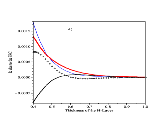
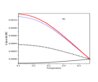
Figure 2: (color online) Normalized critical current due to the SR components, $I_{cSR}$, for the parallel (P) and antiparallel (AP) orientations of magnetization in domains in the middle $H$-layer vs the thickness of the $H$-layer (A) and temperature (B). The thickness of the $h$-layers is assumed to be small ($L_{h}<<\xi_{h}$). The normalized temperature $\tilde{T}$, exchange energy $\tilde{H}$ and thickness $\tilde{L}_{H}$ are measured in units $\Delta_{0}$ and $\xi_{\Delta}=\sqrt{D/\Delta_{0}}$, where $\Delta_{0}=\Delta(T)$ at $T=0$. The lower and upper curves correspond to the P and AP configuration, respectively. The critical current $j_{c}$ is measured in units of its value in a junction with $H=0$ (no exchange field) and normalized length $\tilde{L}_{H}=0.5$. The point and upper thin curves correspond to $\tilde{H}=70$; the lowest and upper thick curves correspond to $\tilde{H}=30$. The normalized temperature (in Fig.A) and thickness $\tilde{L}_{H}$ (in Fig.B) are equal to 0.1 and 0.5; the parameter $\tau_{m}\Delta$ equals 1. The values of the critical current corresponding to $\tilde{H}=30$ are reduced by 10 times.

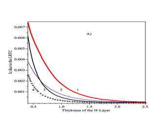
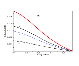
Figure 3: (color online) The same dependence as in Fig.2 for the normalized critical current due the LRTC components, $I_{cLR}$. As in Fig.2, the thickness of the $h$-layers is assumed to be small ($L_{h}<<\xi_{h}$). The normalization units are the same as in Fig.2. The curves are numbered so that: 1 - AP, ($\tilde{H}=30$); 2 - AP (70); 3 - P (30); 4 - P (70).

These formulas show that the critical current density $j_{cSR}$ decays exponentially with increasing the length $L_{H}$ over a short scale of the order $\xi_{H}$. The decrease of the current density $j_{cSR,P}$ with increasing the thickness $L_{H}$ or exchange energy $H$ is accompanied by oscillations GolubovRMP ; BuzdinRMP ; BVErmp . Oscillations in the dependence $j_{cSR,AP}(L_{H},H)$ are absent in the case of antiparallel orientations. The latter behavior was predicted by Blanter and Hekking Blanter who considered antiparallel orientation of magnetization in ferromagnetic domains in a SFS Josephson junction and presented formula for $j_{cSR,AP}$ in the limit $\theta_{H+}\gg 1.$ Eq.(LABEL:jcAnti) generalizes Eq.(26) of Ref.Blanter for the case of arbitrary $\theta_{H\pm}$, i.e. arbitrary $L_{H}.$ A rapid decay and oscillations of the critical Josephson current in SFS or SIFS junctions were observed in many experimental works Ryaz01 ; Ryaz06 ; Kontos ; Blum ; Bauer ; Sellier ; Weides06 ; Weides09 ; Blamire06 ; Shelukhin ; Westerholt ; Birge09 . This oscillatory behaviour was predicted a few decades ago Bulaev ; BuzdinBul .

In Fig.2a and 2b we show the dependence of the normalized critical currents density $I_{cSR}\equiv$ $j_{cSR}(h,H,L_{H})/j_{c}(0,0,L_{H})$ originating from the short-range component (the components $f_{0,3}$) on the thickness of the $H$-layer $L_{H}$ and temperature for the P and AP magnetization orientation. The plots are obtained on the basis of Eqs. (43-LABEL:jcAnti) applicable in the case of thin $h$-layers. We see that in the case of the P orientation the critical current density $j_{c,SR}$ caused by the SRC changes sign with increasing $L_{H},$ while in the case of the AP orientation the current $j_{c,SR}$ is always positive. However, at a fixed $L_{H}$ the current density $j_{cSR}$ decays monotonously with increasing temperature. For a smaller exchange energy the dependence $j_{cSR}(T)$ has another form and may change the sign (see the next subsection).

Note that the critical current for the AP orientation $I_{cSR,AP}$ is always larger that for the P orientation. The critical current $I_{cSR,AP}$ in an SFIFS Josephson junction with the antiparallel magnetization orientation in the F layers may be even exceed the critical current in SIS junction without the F layers provided that the coupling between S and F layers is strong enough ( here I stands for an insulator) BVE01a ; BVErmp .

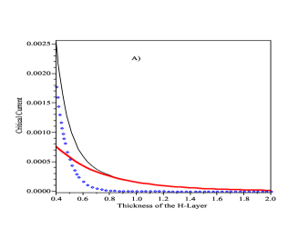
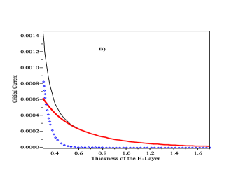
Figure 4: (color online) The dependence of the normalized critical current due to the SR component (point line), LRTC (solid thick line) and the total critical current (solid thin line)on the thickness of the $H$-layer for $\tilde{H}=70$ (A) and $\tilde{H}=170$ (B). The normalized temperature is equal to 0.1. Other parameters are the same as in Fig.2.

The Josephson current $j_{JLR}$ due to the LRTC is found using Eqs. (39, 18,LABEL:A1B1). We obtain

$$j_{JLR}=i\sigma\pi T\gamma_{1}^{2}\sin\alpha_{r}\sin\alpha_{l}\sum_{\omega\geq 0}\frac{Tr\{\hat{\tau}_{3}\hat{f}_{3}(L_{H})\hat{f}_{3}(-L_{H})\}}{\kappa_{\omega}\sinh(2\theta_{H\omega})}$$

(45)

The matrices $\hat{f}_{3}(\pm L_{H})$ are expressed in terms of  the matrices $\hat{f}_{\pm}(\pm L_{H}):$ $\hat{f}_{3}(\pm L_{H})=[\hat{f}_{+}(\pm L_{H})-\hat{f}_{+}(\pm L_{H})]/2.$ Using Eqs.(12-13), we find that $j_{JLR}=j_{cLR}\sin(2\varphi)$. The critical current $j_{cLR}$ in the case of the P and AP orientations is given by

$$j_{cLR,P}=-4\sigma\gamma_{B}^{2}\gamma_{1}^{2}\sin\alpha_{r}\sin\alpha_{l}(2\pi T)$$

$$\times\sum_{\omega\geq 0}\frac{f_{S}^{2}}{\kappa_{\omega}\sinh(2\theta_{H\omega})}ReP_{1}\cdot ReP_{2},$$ (46)

$$j_{cLR,AP}=-\sigma\gamma_{B}^{2}\gamma_{1}^{2}\sin\alpha_{r}\sin\alpha_{l}(2\pi T)$$

$$\times\sum_{\omega\geq 0}\frac{f_{S}^{2}}{\mathcal{D}_{AP}^{2}\kappa_{\omega}\sinh(2\theta_{H\omega})}[P_{3}^{2}-1],$$ (47)

where $P_{1}=\cosh^{2}\theta_{+}/\mathcal{D}_{+},$ $P_{2}=\sinh^{2}\theta_{+}/\mathcal{D}_{+},$ $P_{3}=|\cosh\theta_{+}|^{2}(1+|\tanh\theta_{+}|^{2}Re(\kappa_{+}/\kappa_{-})),$ $\mathcal{D}_{+}$ and $\mathcal{D}_{AP}\equiv\mathcal{D}_{AP+}=\mathcal{D}_{AP-}$ are defined in Eq. (LABEL:Den). Eq. (46) resembles Eqs. (12) and (10) of Refs.BVE03 ; BuzdinHouzet , respectively. Comparing Eq. (46) with Eq.(10) of Ref.BuzdinHouzet one has to have in mind that other boundary conditions and temperatures close to $T_{c}$ are considered in that work. Note that the parameter $(\gamma_{1}/\kappa_{\omega})=(\kappa_{h}L_{h})(\kappa_{h}/\kappa_{\omega})$ may be arbitrary; we assumed that $\kappa_{h}L_{h}\ll 1$, but the parameter $(\kappa_{h}/\kappa_{\omega})$ is large.

In Figs. 3a and 3b we plot the same dependencies as in Figs. 2a and 2b for the critical current $j_{cLR}$ originating from the LRTC. This current decays monotonously with increasing both the temperature and $L_{H}$. Note that the critical current $j_{cLR}$ has the opposite sign to $j_{cSR,AP}$ if $\sin\alpha_{r}\sin\alpha_{l}>0$ and in the case of the AP configuration is always larger than in the case of the P configuration.

In Figs. 4a and 4b we plot the most important dependencies of the $j_{cSR}(T)$ and $j_{cLR}(T)$ as well as the total critical current, $j_{cTot}=$ $j_{cSR}(T)+$ $|j_{cLR}(T)|,$ on the length $L_{H}$ for different magnitudes of the exchange energy $H$. The parameter $p(\alpha_{r},\alpha_{l})\equiv 4\gamma_{1}^{2}\xi_{\Delta}^{2}\sin\alpha_{r}\sin\alpha_{l}$ is taken to be equal to $0.2.$ The value of $H=170\Delta_{0}$ approximately corresponds to the exchange energy in $Co$ ($E_{ex}=309meV,$ see Blamire06 ) used in the experiment Birge . One can see that for $H=70\Delta_{0}$ and $H=170\Delta_{0}$ the critical current is caused by the LRTC at $L_{H}\gtrsim 0.5\xi_{\Delta}$ and at $L_{H}\gtrsim 0.4\xi_{\Delta}$, respectively, where $\xi_{\Delta}=\sqrt{D/\Delta_{0}}$. The latter curve is close to the one observed in Ref.Birge provided we accept $\xi_{\Delta}=10nm$ corresponding to the value of the diffusion coefficient $D$ about $10cm^{2}/s$.

One can say that the obtained results are in a qualitative agreement with experimental data Birge . It is difficult to carry our the quantitatvie comparison because our model is simplified. We admit the standard model in which one neglects the difference in the diffusion coefficients for the major and minor electrons in the ferromagnetic layers although this difference in $Co$ is large. We also assume the diffusive limit for all layers. At the same time, the mean free path in the strong ferromagnet ($Co$) seems to be larger than $\xi_{H}$. In this case the formula for the Josephson current even for one-layer SFS junction becomes rather complicatedBVECrCur .

In addition, the conductivities in all the layers are assumed to be equal whereas in experiment the conductivities in layers ($Cu,Co$ and $PdNi$) are different. The interface resistance $R_{B}$, strictly speaking, is not known and can be only estimated. However, one can see from Eqs.(43-LABEL:jcAnti) that both the ”effective conductivity” $\sigma$ (averaged over all layers) and the averaged interface resistance $R_{B}$ enter the expression for the critical current density $j_{c}$ as a prefactor before the sum. It disappears when we plot the critical current normalized to its value at $h=H=0.$ The most interesting dependence of the critical current $j_{c}$ on temperature and thicknesses $L_{h,H}$ is determined by exponential functions.

We assumed that the proximity effect is weak, that is, the amplitude of the condensate functions in ferromagnets is small. As follows from Eq.(LABEL:Bpm), this means that the parameter $|\gamma_{B}/\kappa_{+}|\approx|\rho L_{h,H}/R_{B}\theta_{+}|\approx|\rho L_{h,H}/R_{B}|\ll 1.$ According to Ref.Birge09 , where a structure similar to that in Ref.Birge (but without strong ferromagnets) was studied, the interface resistance per unit area, $R_{B}=SR_{SF},$ was equal $R_{B}=2.3\cdot 10^{-8}\Omega cm^{2}$ whereas $R_{F}S=\rho_{F}L_{F}\approx 7\cdot 10^{-12}\Omega cm^{2},$ that is, the ratio $R_{F}S/R_{B}\approx 10^{-4}$ is indeed very small, here $S$ is the cross section area of the junction. Taking into account that the resistance of the $h$ and $H$ ($Co$) - layers are comparable, we conclude that the proximity effect in experiment Birge is weak.

As to the value of the critical current, we do not attempt to carry out a quantitative comparison with experimental value because it depends on the ratio $(\rho L/R_{B})^{2}=(R_{F}S/R_{B})^{2}$ which is known only on the order of magnitude. In addition to that, the Josephson junction used in experiment contains many interfaces each of which reduces the proximity effect.

V.2 Arbitrary Thicknesses of the F Layers

In order to calculate the current density $j_{JSR}$, we substitute Eqs.(25-31) into Eq.(38) using the relations $\hat{f}_{0,3}(x)=[\hat{f}_{+}(x)\pm\hat{f}_{+}(x)]/2.$ After simple calculations, we obtain for the critical current density $j_{cSR}$ in the case of the P configuration

$$j_{cSR}=\sigma(2\pi T)\gamma_{B}^{2}\sum_{\omega\geq 0}Re[\frac{f_{S}^{2}}{\kappa_{H+}R(cs/sc)_{+}R(cc/ss)_{+}}]$$ (48)

The critical current density due to the LRTC, $j_{cLR},$ for the case of the arbitrary thicknesses $L_{h,H}$ is found from Eqs.(33-36,39). For the symmetric case ($\alpha_{r}=\alpha_{l}\equiv\alpha\ll 1$) we get

$$j_{cLR}=-\sigma(2\pi T)\gamma_{B}^{2}\alpha^{2}\sum_{\omega\geq 0}\frac{f_{S}^{2}}{\kappa_{\omega}\sinh(2\theta_{\omega})}Im(M)Im(N)$$ (49)

where

$$M=\frac{\sinh\theta_{H+}\cosh\theta_{h\omega}}{R(cs/sc)_{+}}+\frac{\kappa_{\omega}\cosh\theta_{H+}\sinh\theta_{h\omega}}{\kappa_{H+}R(cs/sc)_{+}},$$

(50)

$$N=\frac{\cosh\theta_{H+}\cosh\theta_{h\omega}}{R(cc/ss)_{+}}+\frac{\kappa_{\omega}\sinh\theta_{H+}\sinh\theta_{h\omega}}{\kappa_{H+}R(cc/ss)_{+}},$$

(51)

and $\theta_{\omega}=\theta_{\omega h}+\theta_{\omega H}$. In the antisymmetric case ($\alpha_{r}=-\alpha_{l}\equiv\alpha\ll 1$) the sign of the critical current density should be changed. Thus, in this case the critical current has the same sign as in SNS junction.

Using Eqs.(41-51), we calculate numerically the critical currents $j_{cSR}$ and $j_{cLR}$ for the case of symmetric case ($\alpha_{r}=\alpha_{r}\equiv\alpha\ll 1$) and the P configuration. In Fig. 5a and 5b the dependence of $j_{cSR}$ and $j_{cLR}$ on temperature $T$ is shown for the case when the exchange energies are not very high ($H=2h=10\Delta_{0}$) and the lengths $L_{H,h}$ are small ($L_{h}\approx L_{H}=0.1\xi_{\Delta}$). It is seen that the current $j_{cSR}$ depends on $T$ in a non-monotonic way and can change sign. This type of a non-monotonic temperature dependence was obtained in many works, both experimental Ryaz01 and theoretical (see reviews GolubovRMP ; BuzdinRMP and references therein as well as a recent paper SudboJJ ). The critical current due to the LRTC $j_{cLR}$ decays with increasing $T$ monotonously. Note that a non-monotonic behavior of $j_{cLR}(T)$ was found in Ref. EschrigRev for a half-metallic ferromagnet. In our model, we do not find values of parameters at which this dependence would not be monotonic. However, there is no contradiction between these two results because, as was shown recently EschrigPRL09 , the non-monotonic temperature dependence of the critical Josephson current $I_{cLR}$ takes place only for a sufficiently large exchange energy (comparable with the Fermi energy $\epsilon_{F}$). In our study we assume that both exchange energies, $h,H$, are small in comparison with $\epsilon_{F}$. In a recent work Westerholt10 , the Josephson dc effect was observed in a SFS junction with ferromagnetic $Cu_{2}MnAl$-Heusler alloy as a ferromagnetic layer. In the interval of thicknesses $8nm\lesssim L_{F}\lesssim 10.5nm$ the critical current as a function of $L_{F}$ shows a very slow decay with increasing $L_{F},$ and its temperature dependence was a non-monotonic in this interval of $L_{F}.$

In Fig.6A we show the dependence of $j_{cLR}(L_{h})$ for different exchange energies $h$ setting the angle $\alpha$ equal to $\sqrt{0.1}$. It is seen that the critical current caused by the LRTC has a maximum at $L_{h}\approx\xi_{h},$ that is, the maximum shifts to smaller $\xi_{h}$ with increasing $h$. The same dependence $j_{cLR}(L_{h})$, but for different $H$, is shown in Fig.6B. One can see that the position of the maximum weakly depends on $H.$ A nonmonotonic behaviour of the critical current as a function of $L_{H}$ was observed in experiment Birge .

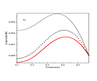
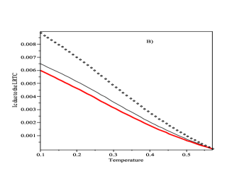
Figure 5: (color online) Temperature dependence of the normalized critical current due to the SR (A) and LRTC (B) components for the P orientation. The upper and lower curves correspond to $\tilde{h}=5$, $\tilde{H}=10$ and to normalized lengths $\tilde{L}_{h}=0.1$ and $\tilde{L}_{h}=0.12$. The point curve corresponds to $\tilde{h}=5,\tilde{H}=10$ and $\tilde{L}_{h}=0.1$. The ”length” $\tilde{L}_{H}=0.1$ and the parameter $\tau_{m}\Delta_{0}=0.1$.

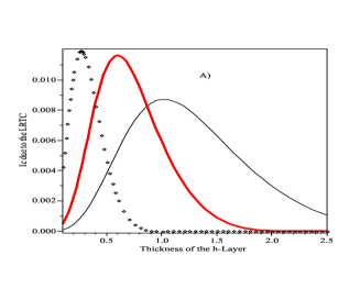
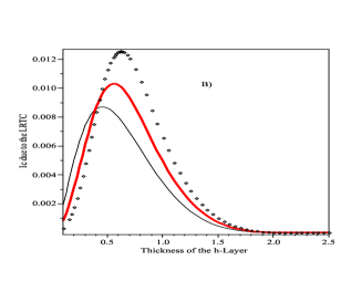
Figure 6: (color online) A) Normalized critical current due to the LRTC as a function of the thickness of the $h$-layer for different exchange energies $h$ for the P orientation. The parameters are: $\tilde{h}=2,5,20$ (solid thin, solid thick and point lines, respectively). The other parameters are $\tilde{H}=50,\tilde{T}=0.25,\tau_{m}\Delta=0.1,\tilde{L}_{H}=0.5$. B) The same dependence for different $\tilde{H}$: $\tilde{H}=5$ (thin solid curve), $\tilde{H}=20$ (thick solid curve) and $\tilde{H}=100$ (point curve). The parameter $\tilde{h}=5$. Other parameters are the same as in Fig.6A. All the curves correspond to the P orientation.

VI Discussion

We have considered the long-range triplet component in an SF’FF’S diffusive Josephson junction with a non-collinear magnetization $M$ orientation in the F’ and F ferromagnetic layers. Assuming that the proximity effect is weak, we have solved the linearized Usadel equation and found the pair wave functions for the short-range (singlet and $S=0$ triplet) and long-range components (the LRTC with $|S|=1$) in the cases of different exchange fields in F’ and F layers, arbitrary temperatures and parallel (antiparallel) $M$ orientation in two domains in the middle F layer.

Our study was motivated by recent experimental results concerning the observation of the LRTC in a multilayered (seven layers between superconductors) Josephson junctions Birge . The model used in our study, although accounting for the properties of the SFS junction used in the experiment Birge , is somewhat simplified. In particular, we solve the Usadel equation in which the difference in transport properties of the minor and major electrons in the F layers was ignored. This approximation is rather crude especially for strong ferromagnets (in $Co$ the diffusion coefficients for the minor and major electrons may differ by an order of magnitude Birge ). Account for different transport properties for electrons with up and down spins leads to a change not only in the boundary condition (4) Belzig+Naz but also in the collision integral by potential impurities BVE02 . The scattering by stationary fluctuations of magnetic moments in the ferromagnetic layers is also taken into account in the simplest way ignoring the spin-orbit interaction Demler .

Thus, the approximations taken by us do not allow a quantitative comparison of the critical current $j_{c}$ measured in experiment and calculated on the basis of the quasiclassical theory within a simplified model.  The formulas for $j_{c}$, Eqs.(43-LABEL:jcAnti), contain an effective conductivity averaged over all layers and effective interface resistance. Even in a simpler case of SFS junctions with a single ferromagnetic layer it is not possible yet to obtain a quantitative agreement between theory based on the quasiclassical theory and experiment Blamire06 ; Birge09 .

Fortunately, both these parameters enter the corresponding formulas as prefactors which disappear when the critical current $I_{c}(T,h,H,L_{h},L_{H})$ is normalized to its value at $h=H=0$. Therefore, the performed study allows one to understand what kind of dependencies of the critical current $I_{c}$ on different parameters ($T,L_{H},L_{h},H,h$) can be obtained in multilayered Josephson SFS junction. If the magnetization in the domains in the F layer is aligned parallel, the critical current $I_{cSR}$ caused by the short-range components oscillates with increasing the thicknesses of the F’ and F layers ($L_{h,H}$). This behavior was predicted in Refs.Bulaev ; BuzdinBul and observed in many experimental works Ryaz01 ; Ryaz06 ; Kontos ; Blum ; Bauer ; Sellier ; Blamire06 ; Weides06 ; Weides09 ; Westerholt ; Birge09 . The formulas obtained in this paper generalize previous theoretical results for $I_{cSR}$ (see reviews GolubovRMP ; BuzdinRMP ; BVErmp and references therein) to the case of different exchange fields in the F’ and F films.

If the magnetization in domains in the F layer are antiparallel, the critical current $I_{cSR}$ decays exponentially in agreement with the results of Ref.Blanter . In both the cases of the parallel and antiparallel orientations the characteristic length for the decay of $I_{cSR}$ is of the order of $\xi_{h,H}$.

The critical current $I_{cLR}$ due to the LRTC decays in both cases with increasing $L_{H}$ and $T$ in a monotonic way on the length of the order of $\xi_{N}.$ For certain values of parameters of the system the total critical current $I_{c}=$ $I_{cSR}+I_{cLR}$ coincides with $I_{cSR}$ at small thickness of the F layer $L_{H}$ and with $I_{cLR}$ at larger $L_{H}$ (see Fig.4). This behavior agrees with the dependence $I_{c}(L_{H})$ observed in the experiment Birge .

As it was predicted in Ref.BVE03 for a F’SFSF’ system and in Ref.BuzdinHouzet for a SF’FF’S system, the current $I_{cLR}$ has a maximum as a function of $L_{h}$ at $L_{h}\sim\xi_{h}$ decaying to zero at large and small $L_{h}$. Thus, the presence of the the F’ layers makes the F layer with a strong ferromagnet “transparent” for the LRTC. Unlike previous theoretical studies, we present a formula for the amplitude of the current $I_{cLR}$ for arbitrary thicknesses $L_{h,H}$, temperatures and exchange fields $h,H$. This allows one to choose optimal parameters for observing the LRTC.

However, it remains unclear how the angle dependence of the critical $j_{cLR}(\alpha_{r,l})$ shows up in the critical current $I_{c}$ observed in experiment. Generally speaking, orientations of the $M$ vectors in F’ and F films are not necessarily the same ($\alpha_{r,l}\neq 0$). If there are domains in the F’ layers, the total critical current $I_{c,Av}$ is determined by averaging the current density $j_{c}$ over the width of the junction as the magnitude and sign of the average $\langle\sin\alpha_{r}\sin\alpha_{l}\rangle$ depends on the number of domains, orientations of the magnetization $M$ in these domains etc. This issue requires a further theoretical and experimental studies.

VII Appendix

The boundary conditions for the matrices $\hat{f}_{0,3}$ follow directly from Eq. (4) and have the form

$$\partial\hat{f}_{3}/\partial x|_{x=\pm L}=\pm\gamma_{B}\hat{f}_{S}|_{x=\pm L},\text{ \ }\partial\hat{f}_{0}/\partial x|_{x=\pm L}=0.$$ (52)

Substituting Eqs. (28,27) into Eqs.(52), we obtain Eqs. (31). The coefficients $C_{h\pm}^{(1,2)}$ are found from the matching conditions of the functions $\hat{f}_{0,3}(x)$ and their derivatives at $x=L_{H}.$ They equal

$$C_{h\pm}^{(1)}=S_{h\pm}^{(1)}\frac{R_{\pm}(sc/cs)}{R_{\pm}(cc/ss)};\text{ }C_{h\pm}^{(2)}=S_{h\pm}^{(2)}\frac{R_{\pm}(ss/cc)}{R_{\pm}(cs/sc)}.$$ (53)

Eqs. (27, 31, 53) determine the form of the function $\hat{f}_{3}(x)$ in Eq. (32). The solution for Eq. (32) is given by the formula

$$\hat{F}_{1}(x)=\hat{F}_{1un}(x)+\hat{F}_{1nun}(x),$$ (54)

where $\hat{F}_{1un}(x)$, $\hat{F}_{1nun}(x)$ are solutions of a homogeneous Eq.(32) (without the R.H.S.) and $\hat{F}_{1nun}(x)$ is a particular solution of this equation. These functions are

$$\hat{F}_{1un}(x)=\hat{\tau}_{2}[a^{(2)}\cosh(\kappa_{\omega}\tilde{x})+b^{(2)}\sinh(\kappa_{\omega}\tilde{x})]$$

$$+\hat{\tau}_{1}[a^{(1)}\cosh(\kappa_{\omega}\tilde{x})+b^{(1)}\sinh(\kappa_{\omega}\tilde{x})]\}$$ (55)

$$\hat{F}_{1nun}(x)=\sin\alpha\sum_{j=1,2}i(-1)^{j}\{\hat{\tau}_{2}S_{hj}^{(2)}[\frac{R_{j}(ss/cc)}{R_{j}(cs/sc)}\cosh(\kappa_{hj}\tilde{x})$$

$$+\sinh(\kappa_{hj}\tilde{x})]+\hat{\tau}_{1}[\frac{R_{j}(sc/cs)}{R_{j}(cc/ss)}\cosh(\kappa_{hj}\tilde{x})+\sinh(\kappa_{hj}\tilde{x})]\}$$

(56)

Matching Eqs.(54-56), we find finally the matrices $\hat{a}_{H}$ and $\hat{b}_{H}$, Eqs. (35-36).

VIII Acknowledgements

We thank SFB 491 for financial support.

References

- (1) J. Bardeen, L.N. Cooper, and J.R. Schrieffer, Phys. Rev. 108, 1175 (1957).
- (2) J.R. Schrieffer, Superconductivity (Benjamin, New York), (1964).
- (3) J.G. Bednorz and K.A. Müller, Z. Phys. 64, 189 (1986).
- (4) C.C. Tsuei, and J.R. Kirtley, Rev. Mod. Phys. 72, 969 (2000).
- (5) D.J. Van Harlingen, Rev. Mod. Phys. 67, 515 (1995).
- (6) A.P. Mackenzie and Y. Maeno, Rev. Mod. Phys. 75, 657 (2003).
- (7) I. Eremin, D. Manske, S.G. Ovchinnikov, and J. F. Annett, Ann. Phys. (Berlin) 13, 149 (2004).
- (8) V.P.Mineev and K.V.Samokhin, Introduction to Unconventional Superconductivity (Gordon and Breach, Amsterdam; 1999).
- (9) V.L. Berezinskii, JETP Lett. 20, 287 (1975).
- (10) A.J. Leggett, Rev. Mod. Phys. 47, 331 (1975).
- (11) D.Vollhardt and P.Wölfle, The superfluid phases of He3 (Taylor and Francis. London, New York, Philadelphia; 1990).
- (12) T.R. Kirkpatrick and D. Belitz, Phys. Rev. Lett. 66, 1533 (1991).
- (13) P. Coleman, E. Miranda, and A. Tsvelik, Phys. Rev. Lett. 70, 2960 (1993).
- (14) E. Abrahams, A.V. Balatsky, J.R. Schrieffer, and P.B. Allen, Phys. Rev. B 47, 513 (1993).
- (15) F.S. Bergeret, A.F. Volkov, K.B. Efetov, Phys. Rev.Lett. 86, 4096 (2001).
- (16) P. G. de Gennes, Rev. Mod. Phys. 36, 225 (1964).
- (17) A.A. Golubov, M.Y. Kupriyanov, and E.Il’ichev, Rev. Mod. Phys. 76, 411 (2004).
- (18) F.S. Bergeret, A.F. Volkov, K.B. Efetov, Rev. Mod. Phys. 77, 1321 (2005).
- (19) A. Buzdin, Rev. Mod. Phys. 77, 935 (2005).
- (20) M. Eschrig, T. Lofwander, T. Champel, J. C. Cuevas, J. Kopu, Gerd Schön, J. Low Temp. Phys. 147, 457, (2007); M. Eschrig, T. Lofwander, Nature Physics 4, 138-143 (2008).
- (21) A.F. Volkov and K.B. Efetov, Phys. Rev. B 72, 184504 (2008).
- (22) A.F. Volkov, Ya.V. Fominov, and K.B. Efetov, Phys. Rev. B 72, 184504 (2005); Ya.V. Fominov, A.F. Volkov, and K.B. Efetov, Phys. Rev. B 75, 104509 (2007).
- (23) V. Braude and Yu. V. Nazarov, Phys. Rev. Lett. 98, 077003 (2007).
- (24) Z. Pajovic, M. Bozovic, Z. Radovic, J. Cayssol, and A. Buzdin, Phys. Rev. B 74, 184509 (2006).
- (25) K. Halterman, O. T. Valls, Physica C 420, 111 (2005).
- (26) Y. Asano, Y. Sawa, Y. Tanaka, and Alexander A. Golubov, Phys. Rev. B 76, 224525 (2007).
- (27) B. Béri, J. N. Kupferschmidt, C. W. J. Beenakker, P. W. Brouwer, Phys.Rev.B 79, 024517 (2009).
- (28) A. F. Volkov, A. Anishchanka, K. B Efetov, Phys. Rev. B 73, 104412 (2006).
- (29) T. Champel, T. Löfwander, M. Eschrig, Phys. Rev. Lett. 100, 077003 (2008).
- (30) Gábor B. Halász, J. W. A. Robinson, M. G. Blamire, James F. Annett, Phys. Rev. B 79, 224505 (2009)
- (31) M. Alidoust, J. Linder, G. Rashedi, T. Yokoyama, and A. Sudbo, Phys. Rev. B 81, 014512 (2010).
- (32) I. Sosnin, H. Cho, V.T. Petrashov, and A.F. Volkov, Phys. Rev. Lett. 96, 157002 (2006).
- (33) R.S. Keizer, S.T.B. Goennenwein, T.M. Klapwijk, G. Miao, G. Xiao, A. Gupta, Nature 439, 825 (2006).
- (34) M. Eschrig, J. Kopu, J.C. Cuevas, and G. Schön, Phys. Rev.Lett. 90, 137003 (2003).
- (35) A.V. Galaktionov, M.S. Kalenkov, and A.D. Zaikin, Phys. Rev. B 77, 094520 (2008).
- (36) Trupti S. Khaire, Mazin A. Khasawneh, W. P. Pratt, Jr., and Norman O. Birge, Phys. Rev. Lett., 104, 137002 (2010)
- (37) M.S. Anwar, M. Hesselberth, M. Porcu, J. Aarts, arXiv:1003.4446.
- (38) Trupti S. Khaire,W. P. Pratt, Jr., and Norman O. Birge, Phys. Rev. B 79, 094523 (2009).
- (39) Y.S. Barash, I.V. Bobkova, and T. Kopp, Phys. Rev. B 66, 140503(R) (2002).
- (40) B. Crouzy, S. Tollis, and D.A. Ivanov, Phys. Rev. B 75, 054503 (2007).
- (41) I. Sperstad, J. Linder, and A. Sudbo, Phys. Rev. B 78, 104509 (2008).
- (42) A.F. Volkov, F.S. Bergeret, K. B. Efetov, Phys. Rev. Lett. 90, 117006 (2003).
- (43) M. Houzet and A. I. Buzdin, Phys. Rev. B 76, 060504(R) (2007).
- (44) A.I. Larkin and Yu.N. Ovchinnikov, in Nonequilibrium Superconductivity, edited by D.N. Langenberg and A.I. Larkin (Elsevier, Amsterdam, 1984).
- (45) J. Rammer and H. Smith, Rev. Mod. Phys. 58, 323 (1986).
- (46) W. Belzig, G. Schoen, C. Bruder, and A.D. Zaikin, Superlattices and Microstructures, 25, 1251 (1999).
- (47) N.B. Kopnin, Theory of Nonequilibrium Superconductivity (Clarendon Press, Oxford, UK, 2001).
- (48) A.V. Zaitsev, JETP 59, 1015 (1984).
- (49) M. Yu. Kupriyanov and V. F. Lukichev, JETP 67, 1163 (1988).
- (50) A. Millis, D. Rainer, and J. A. Sauls, Phys. Rev. B 38, 4504 (1988).
- (51) M. Eschrig, Phys. Rev. B 80, 134511 (2009).
- (52) R. Grein, M. Eschrig, G. Metalidis, and Gerd Schön, Phys. Rev. Lett. 102, 227005 (2009).
- (53) M. S. Kalenkov, A. V. Galaktionov, A. D. Zaikin, Phys. Rev. B 79, 014521 (2009).
- (54) A. Cottet, D. Huertas-Hernando, W. Belzig, Yu. V. Nazarov, Phys. Rev. B 80, 184511 (2009)
- (55) J. Linder and A. Sudbø, Phys. Rev. B 76, 064524 (2007).
- (56) Ya.M. Blanter and F.W. Hekking, Phys. Rev. B 69, 024525 (2004).
- (57) E. A. Demler, G. B. Arnold, and M. R. Beasley, Phys. Rev. B 55, 15174 (1997).
- (58) O. Kashuba, Ya. M. Blanter, V. I. Fal’ko, Phys. Rev. B 75, 132502 (2007).
- (59) F. S. Bergeret, A. F. Volkov,and K. B. Efetov, Phys. Rev. B 75, 184510 (2007).
- (60) D.A. Ivanov and Ya.V. Fominov, Phys. Rev. B 73, 214524 (2006).
- (61) D.A. Ivanov, Ya.V. Fominov, M.A. Skvortsov, and P.M. Ostrovsky, Phys. Rev. B 80,, 134501 (2009).
- (62) V.V. Ryazanov, V.A. Oboznov, A.Yu. Rusanov, A.V. Veretennikov, A.A. Golubov, and J. Aarts, Phys. Rev. Lett. 86, 2427 (2001).
- (63) V.A. Oboznov, V.V. Bolginov, A.K. Feofanov, V.V. Ryazanov, and A.I. Buzdin, Phys. Rev. Lett. 96, 197003 (2006).
- (64) T. Kontos, M. Aprili, J. Lesueur, and X. Grison, Phys. Rev. Lett. 89, 137007 (2002).
- (65) Y. Blum, A. Tsukernik, M. Karpovski, and A. Palevski, Phys. Rev. Lett. 89, 187004 (2002).
- (66) A. Bauer, J. Bentner, M. Aprili, M.L. Della Rocca, M. Reinwald, W. Wegscheider, and C. Strunk, Phys. Rev. Lett. 92, 217001 (2004).
- (67) H. Sellier, C. Baraduc, F. Lefloch, R. Calemczuk, Phys. Rev. Lett. 92, 257005 (2004)
- (68) J. W. A. Robinson, S. Piano, G. Burnell, C. Bell, and M. G. Blamire, Phys. Rev. Lett. 97, 177003 (2006).
- (69) V. Shelukhin, A. Tsukernik, M. Karpovski, Y. Blum, K. B. Efetov, A.F. Volkov, T. Champel, M. Eschrig, T. Lofwander, G. Schon, A. Palevski, Phys. Rev. B 73,1 (2006).
- (70) M. Weides, M. Kemmler, E. Goldobin, H. Kohlstedt, R. Waser, D. Koelle, R. Kleiner, Phys. Rev. Lett. 97, 247001 (2006).
- (71) A. A. Bannykh, J. Pfeiffer, V. S. Stolyarov, I. E. Batov, V. V. Ryazanov, M. Weides, Phys. Rev. B 79, 054501 (2009).
- (72) D. Sprungmann, K. Westerholt, H. Zabel, M. Weides, H. Kohlstedt, J. Phys. D: Appl. Phys. 42, 075005 (2009).
- (73) L.N. Bulaevskii, V.V. Kuzii, and A.A. Sobyanin, JETP Lett. 25, 290 (1977).
- (74) A.I. Buzdin, L.N. Bulaevskii, and S.V. Panyukov, JETP Lett. 35, 178 (1982).
- (75) F.S. Bergeret, A.F. Volkov, K.B. Efetov, Phys. Rev. B 64, 134506 (2001).
- (76) F.S. Bergeret, A.F. Volkov, K.B. Efetov, Phys. Rev.Lett. 86, 3140 (2001).
- (77) F.S. Bergeret, A.F. Volkov, K.B. Efetov, Phys. Rev. B 66, 184403 (2002).
- (78) D. Sprungmann, K. Westerholt, H. Zabel, M. Weides, H. Kohlstedt, arXiv:1003.2082.