The Spiral Modes of the Standing Accretion Shock Instability

Abstract

A stalled spherical accretion shock, such as that arising in core-collapse supernovae, is unstable to non-spherical perturbations. In three dimensions, this Standing Accretion Shock Instability (SASI) can develop spiral modes that spin-up the protoneutron star. Here we study these non-axisymmetric modes by combining linear stability analysis and three-dimensional, time-dependent hydrodynamic simulations with Zeus-MP, focusing on characterizing their spatial structure and angular momentum content. We do not impose any rotation on the background accretion flow, and use simplified microphysics with no neutrino heating or nuclear dissociation. Spiral modes are examined in isolation by choosing flow parameters such that only the fundamental mode is unstable for a given polar index $\ell$, leading to good agreement with linear theory. We find that any superposition of sloshing modes with non-zero relative phases survives in the nonlinear regime and leads to angular momentum redistribution. It follows that the range of perturbations required to obtain spin-up is broader than that needed to obtain the limiting case of a phase shift of $\pi/2$. The bulk of the angular momentum redistribution occurs during a phase of exponential growth, and arises from internal torques that are second order in the perturbation amplitude. This redistribution gives rise to at least two counter rotating regions, with the maximum angular momentum of a given sign approaching a significant fraction of the mass accretion rate times the shock radius squared $(\dot{M}\,r_{\rm shock}^{2}\sim 10^{47}$ g cm² s^-1, spin period $\sim 60$ ms). Nonlinear mode coupling at saturation causes the angular momentum to fluctuate in all directions with much smaller amplitudes.

1. Introduction

The explosion mechanism of massive stars is not well understood at present. Observational and theoretical evidence gathered thus far suggests that this mechanism is intrinsically asymmetric for all stars that form iron cores ($\gtrsim 12M_{\sun}$; see, e.g., Wang & Wheeler 2008, Burrows et al. 2007b and Janka et al. 2007 for recent reviews). Stars that end up with O-Ne-Mg cores are currently found to explode in spherical symmetry via the neutrino mechanism (Kitaura et al. 2006, Burrows et al. 2007a, Janka et al. 2008).

One piece of phenomenology that a successful theory of core-collapse supernovae has to explain is the distribution of pulsar spins at birth. Population synthesis studies of radio pulsars generally assume normal or log-normal distributions with mean values ranging from a few ms (Arzoumanian et al. 2002) to a few $\sim 100$ ms (Faucher-Giguère & Kaspi 2006) in order to reproduce observations. This large range is due to the different assumptions made about input physics, such as the shape of the radio beam (e.g., Faucher-Giguère & Kaspi 2006). Independent constraints that combine Chandra, XMM, and Swift observations of historic supernovae with an empirical correlation between X-ray luminosity and spin down power tend to rule out a large pulsar population with initial periods $\leq 40$ ms (Perna et al. 2008). On the other hand, current stellar evolution calculations that account for magnetic torques predict, using conservation of angular momentum and an assumption for the mass cut, neutron star birth periods $\lesssim 10$ ms (Heger et al. 2005). However, these models suffer from large uncertainties in the input physics, which could also lead in principle to very slowly rotating pulsars (Spruit & Phinney 1998). Axisymmetric core-collapse calculations indicate that there is an almost linear mapping between the rotation rate of the iron core and that of the resulting protoneutron star, with no robust braking mechanism in sight to bring the implied fast neutron star spins to values more in agreement with observations (Ott et al. 2006).

If most presupernova cores turn out to rotate slowly, then there is an alternative mechanism to generate periods $\gtrsim 50$ ms, which arises from instabilities in the supernova shock itself (Blondin & Mezzacappa 2007). Axisymmetric core-collapse supernova simulations that include neutrino transport and microphysics to several degrees of approximation find that the stalled postbounce shock undergoes large scale oscillatory motions that break the spherical symmetry of the system (Burrows et al. 1995; Janka & Mueller 1996; Mezzacappa et al. 1998; Scheck et al. 2006; Ohnishi et al. 2006; Buras et al. 2006b, a; Burrows et al. 2006, 2007c; Scheck et al. 2008; Murphy & Burrows 2008; Ott et al. 2008; Marek & Janka 2009; Suwa et al. 2009). When neutrino driven convection is suppressed, the instability of the shock persists in the form of an overstable sloshing cycle, with the most unstable modes having Legendre indices $\ell=1$ and $2$ (Blondin et al. 2003; Blondin & Mezzacappa 2006). In the limit of short wavelength, this so-called Standing, Spherical, or Stationary Accretion Shock Instability (SASI) is driven by an interplay between advected and acoustic perturbations (Foglizzo et al. 2007). There is no conclusive proof yet on the mechanism behind long wavelength modes, although considerations of the timescales (Fernández & Thompson 2009b) and the case of planar geometry (Foglizzo 2009; Sato et al. 2009) point to the advective-acoustic cycle as a relevant component. The SASI is weakened when rotation becomes dynamically important (e.g., Ott et al. 2008).

Three-dimensional simulations of the SASI have found that a spiral type of mode can develop, causing the flow to divide itself into at least two counter-rotating streams, leading to angular momentum redistribution (Blondin & Mezzacappa 2007). Blondin & Mezzacappa (2007) find that this process can spin-up a canonical neutron star to a period of $\sim 50$ ms after $\sim 0.1M_{\sun}$ of material is accreted. Aside from the fact that this spin period is comparable to that obtained by population synthesis calculations, the most interesting results of Blondin & Mezzacappa (2007) are that (i) no progenitor rotation is required for this mechanism to operate and, (ii) for weak progenitor rotation, this instability dominates the spin-up of the protoneutron star, imparting it along a different axis.

One of the key questions that remains to be answered is how easy it is to excite these spiral modes. In contrast to Blondin & Mezzacappa (2007) and Blondin & Shaw (2007), the findings of Iwakami et al. (2008a), Iwakami et al. (2009a), and Iwakami et al. (2009b) suggest that with no rotation in the upstream flow, these modes are difficult to excite. Yamasaki & Foglizzo (2008) find that, indeed, for a cylindrical accretion flow with rotation, prograde spiral modes have a higher growth rate than retrograde ones. They attribute this to a Doppler shift of the mode frequency induced by rotation. Part of the difficulty in comparing numerical results on this instability is that they have been obtained using different microphysics, numerical methods, and coordinate systems, and that the three-dimensional structure of these linear eigenmodes remains as of yet unexplored. The work of Blondin & Shaw (2007) examined spiral SASI modes with time-dependent hydrodynamical simulations restricted to a polar wedge around the equatorial plane. They found that sloshing and spiral modes are closely related, because the pressure perturbation rotates with the same frequency as a sloshing mode of the same Legendre index, and because by combining two counter-rotating spirals, the flow field of a sloshing mode is recovered. The work of Iwakami et al. (2009b) also identified sloshing modes as the superposition of two counter-rotating spirals.

The aim of this paper is to better understand spiral modes in the linear and nonlinear phase, particularly their three-dimensional spatial structure and angular momentum content.

The structure of axisymmetric sloshing eigenmodes has been obtained previously through linear stability analysis (Foglizzo et al. 2007), and verified to high precision with time-dependent axisymmetric hydrodynamic simulations (Fernández & Thompson 2009b). Starting from the findings of Blondin & Shaw (2007), we show that spiral modes are most easily understood as sloshing modes out of phase. Their spatial structure is built using solutions to the differential system of Foglizzo et al. (2007), and their evolution is compared with results of time-dependent hydrodynamic simulations using Zeus-MP (Hayes et al. 2006). In our calculations we do not add rotation to the flow anywhere, and employ an ideal gas equation of state, parametric cooling, and point-mass gravity, with no heating or nuclear dissociation below the shock.

One of our main findings is that it is relatively simple to create spiral modes out of sloshing modes by changing their numbers, relative phases, and amplitudes, covering a broader parameter space than the limiting cases where the amplitudes are equal and the relative phase is $\pi/2$. These modes survive to large amplitudes, resulting in a significant angular momentum redistribution below the shock. We set aside for now the question of whether this coherent superposition of sloshing modes is able to develop in a more realistic core-collapse context, where three-dimensional, nonlinear turbulent convection may likely act as a forcing agent (Fernández & Thompson 2009a). We revisit this issue in the discussion section.

We also find that the bulk of the angular momentum redistribution generated by a spiral mode occurs during the phase of exponential growth. This spin-up of the flow arises from internal torques that are second order in the perturbation amplitude, and results in angular momenta of a characteristic magnitude at saturation. Non-linear mode coupling causes the angular momentum flux to become stochastic, fluctuating in all directions with an amplitude much smaller than that achieved during exponential growth.

The structure of this paper is the following. In Section 2 we describe the physical model used, and summarize the most important elements that enter the linear stability calculation and time-dependent simulations, with details deferred to the Appendices. Section 3 describes how spiral modes can be constructed by superposing sloshing modes out of phase, and explores some of their features. Section 4 contains the results of time-dependent simulations of these modes, including both linear and nonlinear development. We conclude by summarizing our findings and discussing their implications for more realistic core-collapse models and neutron star spins.

2. Methods

2.1. Physical Model

The physical system consists of a steady-state, standing spherical accretion shock at a radial distance ${r_{\rm s0}}$ from the origin. Below the shock, the material settles subsonically onto a star of radius $r_{*}$ and mass $M$ centered at the origin of the coordinate system. This settling is mediated by a cooling rate per unit volume that mimics neutrino emission due to electron capture, $\mathscr{L}\propto p^{3/2}\,\rho$, with $p$ the pressure and $\rho$ the density (e.g., Blondin & Mezzacappa 2006, Fernández & Thompson 2009b). In all the cases studied here, cooling is relevant only in a narrow region – of order a pressure scale height – outside the accretor. Upstream of the shock, the fluid is supersonic, with incident Mach number $\mathcal{M}_{1}=5$ at $r={r_{\rm s0}}$, and has a vanishing energy flux. Upstream and downstream solutions are connected by the Rankine-Hugoniot jump conditions. The equation of state is that of an ideal gas of adiabatic index $\gamma=4/3$, and the self gravity of the flow is neglected. The equations describing this steady flow are presented in §A.1. The model was first developed by Houck & Chevalier (1992) to study accretion onto compact objects, and subsequently used by Blondin et al. (2003), Blondin & Mezzacappa (2006), Foglizzo et al. (2007), Blondin & Mezzacappa (2007), Blondin & Shaw (2007), and Fernández & Thompson (2009b) as a minimal approximation to the postbounce stalled shock.

In contrast to Fernández & Thompson (2009b), we do not include here the effects of nuclear dissociation at the shock. This is a significant energy sink in the system, changing the Mach number and density below the shock for fixed upstream conditions, and hence affecting the linear modes of the SASI. Nevertheless, as our goal here is to characterize the basic behavior of the instability in three dimensions, we aim at keeping the calculations as simple as possible.

Neutrino heating is also neglected, in order to suppress convection in the flow, as originally done by Blondin et al. (2003). Since most of the flow below the shock is adiabatic, the entropy profile is flat and hence marginally unstable to overturns triggered by the SASI itself.

We adopt a system of units normalized to the shock radius ${r_{\rm s0}}$, the free-fall velocity at this radius $v_{\rm ff0}=\sqrt{2GM/{r_{\rm s0}}}$, and the upstream density $\rho_{1}$ (Fernández & Thompson 2009b). Numerical values relevant for the stalled shock phase of core collapse supernovae are $r_{\mathrm{s0}}\sim 150$ km, $v_{\mathrm{ff}}(r_{\rm s0})\sim 4.8\times 10^{9}M_{\mathrm{1.3}}^{1/2}\,(r_{\rm s0}/150~{}{\rm km})^{-1/2}$ km s^-1, $t_{\mathrm{ff}}\equiv r_{\mathrm{s0}}/v_{\mathrm{ff}}\sim 3.1\,M_{\mathrm{1.3}}^{-1/2}\,(r_{\rm s0}/150~{}{\rm km})^{3/2}$ ms, and $\rho_{1}\sim 4.4\times 10^{7}\dot{M}_{\mathrm{0.3}}\,M_{\mathrm{1.3}}^{-1/2}\,(r_{s0}/150~{}{\rm km})^{-3/2}$ g cm^-3 (assuming a strong shock), where the mass accretion rate has been normalized to $\dot{M}=0.3\,\dot{M}_{\mathrm{0.3}}\,M_{\odot}$ s^-1. We will express quantities involving angular momentum in terms of $\dot{M}{r_{\rm s0}}\simeq 4\pi\times 10^{46}(r_{\rm s0}/150~{}{\rm km})^{2}\dot{M}_{\mathrm{0.3}}$ g cm² s^-1.

2.2. Linear Stability Analysis

To obtain linear SASI eigenmodes and eigenfrequencies, we solve the differential system of Foglizzo et al. (2007), the results of which agree with time-dependent axisymmetric hydrodynamic simulations to high precision (Fernández & Thompson 2009b). The relevant equations are described in detail in Appendix A; here we summarize the main elements of the calculation. The eigenvalue problem is formulated in terms of perturbation variables that are conserved when advected. These are the perturbed mass flux $h=\delta\rho/\rho+\delta v_{r}/v_{r}$, Bernoulli flux $f=v_{r}\delta v_{r}+\delta c^{2}/(\gamma-1)$, entropy $\delta S=(\gamma-1)^{-1}\left[\delta p/p-\gamma\delta\rho/\rho\right]$, and an entropy-vortex combination $\delta K=r^{2}\mathbf{v}\cdot(\nabla\times\delta\mathbf{w})+\ell(\ell+1)(p/\rho)\delta S$ (see also eq. [A33]), with $c^{2}=\gamma p/\rho$, $\mathbf{v}$ the velocity, and $\mathbf{w}$ the vorticity. Perturbations are decomposed in Fourier modes in time and spherical harmonics in the angular direction, having the general form

$$\delta q=\delta\tilde{q}(r)\,e^{-i\omega t}\,Y_{\ell}^{m}(\theta,\phi),$$ (1)

where $\delta\tilde{q}(r)$ is the complex amplitude, $Y_{\ell}^{m}$ is a spherical harmonic, and the complex frequency satisfies $\omega=\omega_{\rm{osc}}+i\omega_{\rm{grow}}$. This choice results in all thermodynamic variables along with $\delta v_{r}$ being proportional to $Y_{\ell}^{m}$ (corresponding to spheroidal modes, e.g. Andersson et al. 2001). The transverse components of the velocity involve angular derivatives of the $Y_{\ell}^{m}$, and have the same radial amplitude (Appendix A),

$$\delta v_{\theta} = \delta\tilde{v}_{\Omega}(r)\,e^{-i\omega t}\,\frac{\partial}{\partial\theta}Y_{\ell}^{m}(\theta,\phi)$$ (2)

$$\delta v_{\phi} = \delta\tilde{v}_{\Omega}(r)\,e^{-i\omega t}\,\frac{1}{\sin\theta}\frac{\partial}{\partial\phi}Y_{\ell}^{m}(\theta,\phi).$$ (3)

The system of ordinary differential equations that determines the complex amplitudes is independent of the azimuthal number $m$ of the mode. Boundary conditions at the shock are expressed in terms proportional to the shock displacement $\Delta\xi$, or the shock velocity $\Delta v=-i\omega\Delta\xi$. By imposing $\delta\tilde{v}_{r}(r_{*})=0$ at the inner boundary, a complex eigenvalue $\omega$ is obtained for a given set of flow parameters. For each $\ell$, a discrete set of overtones is obtained, which are related to the number of nodes in the radial direction (Foglizzo et al. 2007; Fernández & Thompson 2009b). The resulting eigenmodes have both real and imaginary eigenfrequencies.

For fixed $\gamma$, $\mathcal{M}_{1}$, and functional form of the cooling function, the eigenfrequencies of the SASI depend only on the relative size of the shock and accreting star, quantified by the ratio $r_{*}/{r_{\rm s0}}$. Time-dependent studies of individual SASI modes are possible by choosing model parameters such that only the fundamental mode is unstable, for a given $\ell$. Based on the fact that the relevant modes in more realistic core-collapse simulations are $\ell=1$, and $2$, we adopt two configurations for single-mode studies: $r_{*}/{r_{\rm s0}}=0.5$ for $\ell=1$, and $r_{*}/{r_{\rm s0}}=0.6$ for $\ell=2$ (see Foglizzo et al. 2007 and Fernández & Thompson 2009b for more extended parameter studies of the SASI eigenfrequencies). In addition, we explore a configuration with a larger postshock cavity, $r_{*}/{r_{\rm s0}}=0.2$, to more closely resemble actual stalled supernova shocks. In this case unstable overtones of $\ell=1$ and $\ell=2$ are present.

To facilitate visualization, and unless otherwise noted, we employ the real representation of spherical harmonics. For $\ell=1$, one has

$$Y_{1}^{0} = \sqrt{\frac{3}{4\pi}}\cos\theta$$ (4)

$$Y_{1}^{1} = \sqrt{\frac{3}{4\pi}}\sin\theta\,\cos\phi$$ (5)

$$Y_{1}^{-1} = \sqrt{\frac{3}{4\pi}}\sin\theta\,\sin\phi.$$ (6)

This basis is entirely equivalent to the one involving complex exponentials in azimuth (e.g., Arfken & Weber 2005), but has a straightforward interpretation: equations (4), (5), and (6) are dipoles in the z-, x-, and y-directions, respectively. For $\ell=2$, we have

$$Y_{2}^{0} = \sqrt{\frac{5}{4\pi}}\frac{1}{2}\left(3\cos^{2}\theta-1\right)$$ (7)

$$Y_{2}^{1} = \sqrt{\frac{15}{4\pi}}\sin\theta\cos\theta\,\cos\phi$$ (8)

$$Y_{2}^{-1} = \sqrt{\frac{15}{4\pi}}\sin\theta\cos\theta\,\sin\phi$$ (9)

$$Y_{2}^{2} = \sqrt{\frac{15}{16\pi}}\sin^{2}\theta\,\cos 2\phi$$ (10)

$$Y_{2}^{-2} = \sqrt{\frac{15}{16\pi}}\sin^{2}\theta\,\sin 2\phi,$$ (11)

corresponding to the usual z-symmetric quadrupole ($Y_{2}^{0}$), and a series of 4-striped ”beach balls” with alternating polarity and symmetry axis along $\hat{x}$ ($Y_{2}^{1}$), $\hat{y}$ ($Y_{2}^{-1}$), and $\hat{z}$ ($Y_{2}^{\pm 2}$).

Whenever necessary, we will denote the traditional complex spherical harmonics as $\Upsilon_{\ell}^{m}$.

2.3. Time Dependent Numerical Simulations

We perform time-dependent hydrodynamic calculations to verify the evolution of linear SASI eigenmodes in three dimensions, covering the linear and nonlinear phases. To this end, we employ the publicly available code Zeus-MP (Hayes et al. 2006), which solves the Euler equations using a finite difference algorithm that includes artificial viscosity for the treatment of shocks. The default version of the code supports an ideal gas equation of state and point mass gravity. We have extended it to account for optically thin cooling and a tensor artificial viscosity, for a better shock treatment in curvilinear coordinates (e.g., Stone & Norman 1992, Hayes et al. 2006, Iwakami et al. 2008a). Issues associated with implementing the latter are discussed in Appendix B.

The initial conditions are set by the steady-state accretion flow used in linear stability calculations. To prevent runaway cooling at the base of the flow, we impose a gaussian cutoff in the cooling with entropy (Fernández & Thompson 2009b). The normalization of the cooling function is adjusted so that the Mach number at the surface of the accreting star is $\mathcal{M}\sim 10^{-2}$.

Spherical polar coordinates ($r,\theta,\phi$) are used , covering the whole sphere minus a cone of half-opening angle $5$ degrees around the polar axis. This prescription does not significantly alter the flow dynamics, and ameliorates the severe Courant-Friedrichs-Lewy restriction around the polar axis (H-Th. Janka, private communication). We present convergence studies in Appendix B showing that only $\sim 10\%$ differences relative to using the full sphere are introduced with this prescription. Cells are uniformly spaced in the polar and azimuthal directions, while ratioed in radius. The choice of grid spacing is key to a achieve a stable background solution and to adequately capture linear growth rates, while minimizing the computational cost. The radial size of the cells at $r=r_{*}$, $\Delta r_{\rm min}$, determines how stable the unperturbed shock remains, because near hydrostatic equilibrium needs to be maintained. At the shock, the angular size determines how well growth rates are captured. Based on numerical experiments, we have found that $\Delta r_{\rm min}<10^{-3}{r_{\rm s0}}$ is required to obtain a stable shock within $500$ dynamical times, and that 36 cells in the polar direction is the minimum needed to obtain a clean shock oscillation ($\omega_{\rm osc}$ within $\lesssim 10\%$ and $\omega_{\rm grow}$ within $\sim 20\%$ from the linear stability value; convergence tests are presented in Appendix B). We choose the ratio of radial spacing so that $\Delta r={r_{\rm s0}}\Delta\theta$ at the shock radius ${r_{\rm s0}}$, and $\Delta\phi=\Delta\theta$, resulting in a total of $56$ radial ($\ell=1$), $48$ polar, and $96$ azimuthal cells. For $\ell=2$, we use $28$ ratioed cells in radius from $r_{*}$ to ${r_{\rm s0}}$, and then use a uniform radial spacing until the outer boundary. This choice of grid spacing is made because the tensor artificial viscosity behaves best when applied over the longest cell dimension (e.g., Stone & Norman 1992), and hence choosing the three cell dimensions as equal as possible results in nearly isotropic dissipation except near the polar axis. In addition, we perform one simulation at double the resolution in all dimensions (e.g., 128x96x192) to test the robustness of our results. This resolution approaches values comparable to existing two-dimensional simulations, and can better capture the parasitic instabilities that mediate the saturation of the instability (Guilet et al. 2010). In Table 1 we summarize the modes evolved. With the exception of the high-resolution model (R5_L1P2_HR), all simulations were carried out until at least $200{t_{\rm ff0}}$, well into the nonlinear phase.

Table 1Models Evolved.

Model	$r_{*}/{r_{\rm s0}}$	Perturbation	Resolution
r5_L1_LR(c)	0.5	Shell, $\ell=1$	$\phantom{1}56\times 48$
r5_L1_HR(c)	0.5	Shell, $\ell=1$	$112\times 96$
R2_L11f(c)	0.2	Shells, $\Phi=\pi/2$	$\phantom{1}56\times 48\times 96$
R2_L11h(c)	0.2	Shells, $\Phi=\pi/2$	$\phantom{1}56\times 48\times 96$
R5_L11x	0.5	Shell, $Y_{1}^{1}$ only	$\phantom{1}56\times 48\times 96$
R5_L11P2(c)	0.5	Shells, $\Phi=\pi/2$	$\phantom{1}56\times 48\times 96$
R5_L11P4	0.5	Shells, $\Phi=\pi/4$	$\phantom{1}56\times 48\times 96$
R5_L11P8	0.5	Shells, $\Phi=\pi/8$	$\phantom{1}56\times 48\times 96$
R5_L11_HR	0.5	Shells, $\Phi=\pi/2$	$112\times 96\times 192$
R5_RAN	0.5	Random Pressure 1%	$\phantom{1}56\times 48\times 96$
R6_L21P2(c)	0.6	Shells, $\Phi=\pi/2$	$(28+44)\times 48\times 96$
R6_L21P4	0.6	Shells, $\Phi=\pi/4$	$(28+44)\times 48\times 96$
R6_L21P8	0.6	Shells, $\Phi=\pi/8$	$(28+44)\times 48\times 96$
R6_L22P2(c)	0.6	Shells, $\Phi=\pi/2$	$(28+44)\times 48\times 96$
R6_L22P4	0.6	Shells, $\Phi=\pi/4$	$(28+44)\times 48\times 96$
R6_L22P8	0.6	Shells, $\Phi=\pi/8$	$(28+44)\times 48\times 96$

The boundary conditions are reflecting at the inner radial boundary ($r=r_{*}$), periodic in the $\phi$ direction, reflecting at the polar boundaries ($\theta=\{0,\pi\}$ minus the cutout), and set equal to the upstream flow at the outer radial boundary ($r=4{r_{\rm s0}}$). The use of tensor artificial viscosity prevents the appearance of a numerical instability at the poles of the shock, as described by Iwakami et al. (2008b). This carbuncle instability (Quirk 1994) arises within a few dynamical times if the standard VonNeumann & Richtmyer (1950) prescription is used. However, even when including the tensor viscosity, we have found that a different numerical instability develops around the polar axis when reflecting boundary conditions and the full sphere are used. This is due to the fact that a wake is generated by the reflecting axis when the sloshing modes reach a large amplitude, resulting in a different radial velocity profile at opposite sides of the polar axis. The azimuthal velocity then develops a sawtooth instability around the axis. The cutout improves (but does not completely suppress) the development of this instability, to the point where it does not significantly alter the flow dynamics.

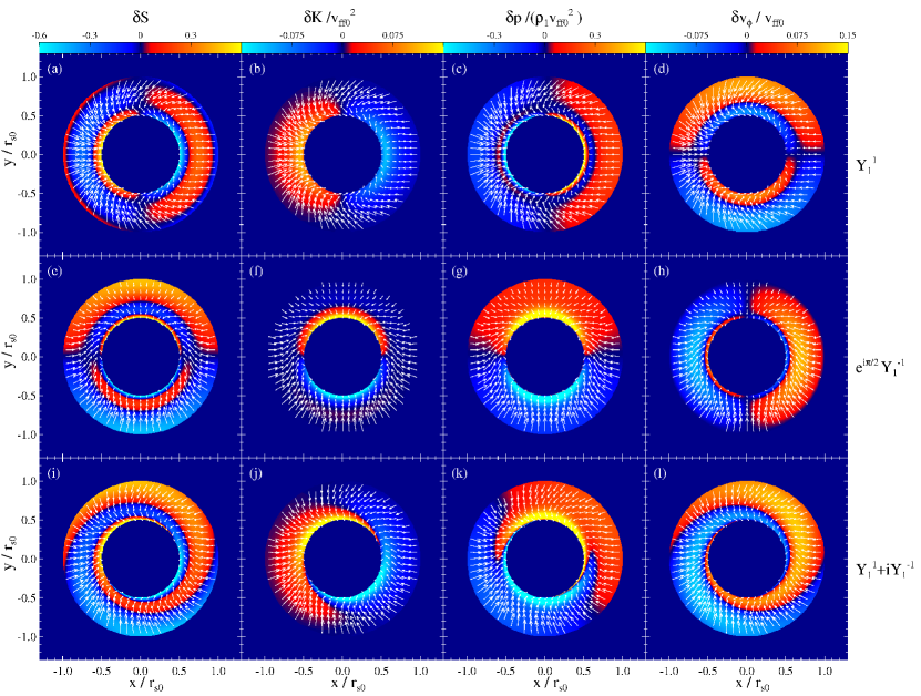
Figure 1.— Real part of perturbed quantities from linear stability analysis, showing how transverse sloshing modes out of phase combine to create a $\ell=1$, $m=1$ spiral mode at the equatorial plane ($z=0$). The top, middle, and bottom rows show the $Y_{1}^{1}$ mode at $t=0$, the $Y_{1}^{-1}$ mode displaced $\pi/2$ in phase, and their sum, respectively (real spherical harmonics are given by eqns. [4]-[6]). From left to right, columns show the entropy, entropy-vortex, pressure, and azimuthal velocity perturbation for a shock displacement amplitude $\Delta\tilde{\xi}=0.25{r_{\rm s0}}$ (§2.2 and Appendix A). White arrows show the perturbed velocity profile. The size of the postshock cavity is $r_{*}/{r_{\rm s0}}=0.5$, and only the fundamental mode is unstable. Note that only the region below the unperturbed shock position is shown. The electronic version of the article contains an animated version of this figure (real frequency only).

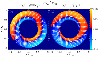
Figure 2.— Effect of changing the relative phase (left) and amplitude (right) relative to the $\ell=1$, $m=1$ spiral in Figure 1l. Shown is the perturbed azimuthal velocity from the linear eigenmodes at $z=0$. The left panel has a phase difference $\Phi=\pi/8$ with equal amplitudes, while the right panel decreases the amplitude of $Y_{1}^{-1}$ by 1/2, with a phase difference of $\pi/2$. The electronic version of the article contains an animated version of this figure (real frequency only).

3. Superposition of Linear Eigenmodes

Understanding of spiral SASI modes becomes easier when the real representation of spherical harmonics is used (eqns. [4]-[11]). For $\ell=1$, they correspond to the familiar sloshing modes, axisymmetric relative to the three cartesian coordinate axes. When viewed this way, the fact that the eigenfrequencies for a given $\ell$ are independent of azimuthal number $m$ is natural, as any of these elementary modes is equally likely to arise in a spherically symmetric accretion flow (see, e.g., Binney & Tremaine 2008 for a more rigorous argument). When excited in phase, any linear combination of these sloshing modes will result in a new sloshing mode that is symmetric around some axis.

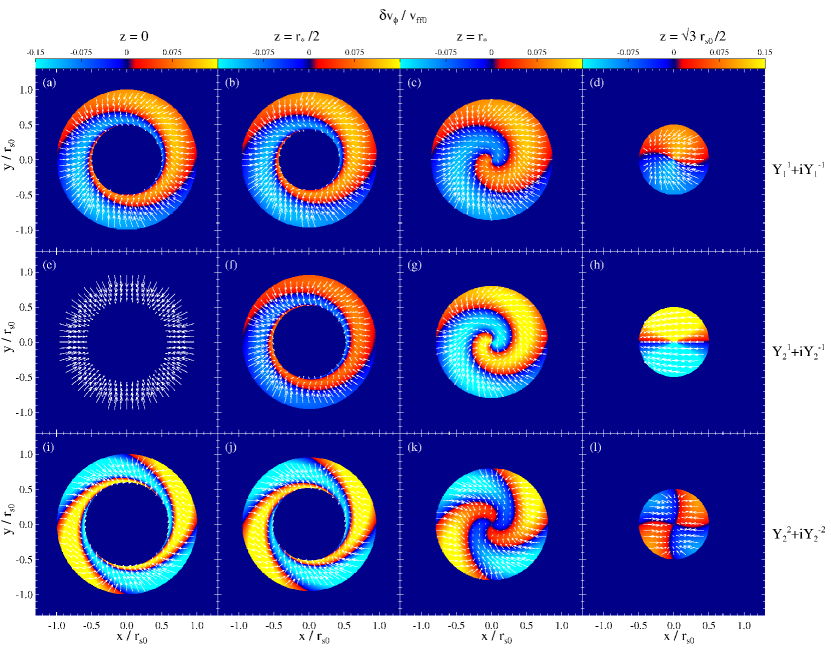
Figure 3.— Real part of the perturbed azimuthal velocity from linear stability, showing the three-dimensional structure of spiral modes for different combinations of $\ell$ and $m$. The top, middle, and bottom rows show $Y_{1}^{1}+iY_{1}^{-1}$, $Y_{2}^{1}+iY_{2}^{-1}$, and $Y_{2}^{2}+iY_{2}^{-2}$, all at $t=0$, respectively. From left to right, columns show different elevations above the equatorial plane. The fractional stellar size is $r_{*}/{r_{\rm s0}}=0.5$ for $\ell=1$ and $r_{*}/{r_{\rm s0}}=0.6$ for $\ell=2$, so that only the fundamental mode is unstable. The equatorial plane of the $Y_{2}^{\pm 1}$ mode (panel e) has only radial flow.

Spiral modes arise whenever two or more of these “basis” sloshing modes are excited out of phase. The familiar $\ell=1$, $m=\pm 1$ spirals corresponds to $Y_{1}^{1}\pm iY_{1}^{-1}$, or x- and y-symmetric sloshing modes that are $\pm\pi/2$ out of phase with each other, and that have the same amplitude, akin to two transverse and out-of-phase harmonic oscillators describing circular motion. Aside from the exponential growth in amplitude, this gives rise to a static spiral pattern that rotates with the angular frequency of the oscillators. This type of spiral motion was suggested by Lin & Shu (1964) to explain the morphology of spiral arms in galaxies, and is also well-known in stellar pulsation theory (e.g., Unno et al. 1989).

Figure 1 shows, side-by-side, the real part of the entropy, entropy-vortex, pressure, and azimuthal velocity perturbation in the equatorial plane ($z=0$), with the total velocity field superimposed. Shown are the fundamental modes $Y_{1}^{-1}$, $\exp(i\pi/2)\,Y_{1}^{-1}$, and the sum of them, for a shock displacement amplitude $\Delta\tilde{\xi}=0.25{r_{\rm s0}}$ (an animated version of the figure is available in the online version of the article). In sloshing modes, the entropy eigenmodes consist of annular regions of alternating polarity that extend over half a circle in azimuth for $\ell=1$, and which are advected with the background flow. The perturbed fluid moves towards regions of low-entropy, which generally coincide with underpressures. The entropy-vortex perturbation ($\delta K$) has opposite polarity than $\delta S$. When combined $\pi/2$ out-of-phase, a spiral pattern is created in $\delta S$, $\delta K$, and $\delta v_{\phi}$. The pressure, however, has a different behavior. In a sloshing mode, it propagates outwards, as can be seen in the animated version of Figure 1. The latter suggests that pressure perturbations arise in response to negative entropy perturbations, which affect the cooling and thus hydrostatic equilibrium (as in the case of $\ell=0$ modes, Fernández & Thompson 2009b). The source terms in the differential system (eqns. [A8]-[A11]) are such that cooling terms are comparable to terms proportional to $\omega$ for fundamental modes (which have the lowest $|\omega|$ for a given $\ell$), decreasing their relative contribution for higher overtones as $\omega$ increases in magnitude. When combined $\pi/2$ out-of-phase, the pressure perturbations from sloshing modes result in two almost half-circular regions of opposite polarity oriented towards the center of the prograde and retrograde fluid streams. As the amplitude grows, a protuberance and depression arise at opposite sides of the shock, following the pressure perturbation (§4). The overall flow structure rotates with a period equal to the oscillation frequency of the sloshing modes.

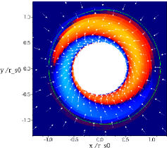
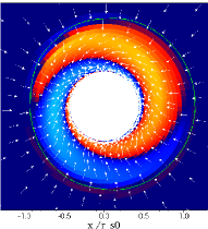
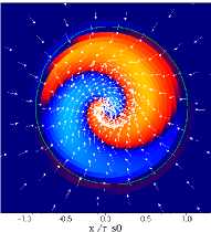
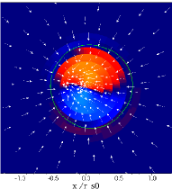
Figure 4.— Azimuthal velocity in a snapshot of model R5_L11P2 at time $t=33{t_{\rm ff0}}$. Units and color table are the same as in Figure 3, and panels from left to right correspond to the same altitudes above the equator. The ratio of stellar to shock radius is $r_{*}/{r_{\rm s0}}=0.5$, for which only the fundamental $\ell=1$ mode is unstable. Despite the relatively coarse grid resolution, the agreement with the linear eigenmodes is excellent. The green contour shows the surface with internal pressure equal to $0.1\rho_{1}v_{\rm ff0}^{2}$. An animated version of this figure is available in the online version of the article.

From the previous discussion, it can be seen that spiral modes need not be limited to the x-y plane, a phase shift of $\pi/2$, or to have equal amplitudes. Panel (a) of Figure 2 shows the effects of decreasing the phase difference from $\pi/2$ to $\pi/8$ relative to the standard case shown in panel (l) of Figure 1. The spiral pattern is still apparent, though not static anymore. Indeed, the animated version of Figure 2 shows that it is in fact episodic, arising whenever the two sloshing modes interact constructively. Panel (b) of Figure 2 shows what happens when the amplitudes are not the same: again, the spiral pattern is still distinguishable, although more irregular. We take these results as an indication that a more general class of spiral-like modes can be obtained by combining sloshing modes in different ways. This means that a larger region of parameter space (number of modes, relative phase, relative amplitude) of initial perturbations can result in spiral-like behavior of the shock compared with the limiting case of $\pm\pi/2$ phase or equal amplitudes. In §4 we show that in fact these modes survive in the nonlinear phase, leading to angular momentum redistribution below the shock (albeit smaller in magnitude than a phase difference of $\pi/2$).

Adding a third sloshing mode in the z-direction ($Y_{1}^{0}$) results in a 45 degree tilt of the “spiral plane” relative to the equator. The azimuthal and polar angles determining the normal to this plane are set by the phase and amplitude of this mode relative to their transverse counterparts, respectively. One can thus immediately see that the torque imparted to the star by nonlinear spiral modes is in a direction set by the way the instability is excited. This conclusion agrees with the results of Blondin & Mezzacappa (2007).

In the parameter regime relevant to core-collapse supernovae, quadrupolar modes are also significant. As with the dipolar case, each of these corresponds to an elementary sloshing SASI mode, which can be combined and excited in phase to generate a sloshing mode along an arbitrary axis. Spiral modes are again generated by exciting at least two of these basic modes out-of-phase. Figure 3 compares the perturbation to the azimuthal velocity for dipolar and quadrupolar spiral modes at different altitudes from the equatorial plane. The $|m|=\ell$ modes preserve their spiral structure from pole to pole, while the $|m|<\ell$ case has a purely radial flow at the equator, and dipolar spiral flows above and below. These dipolar spirals are 180 degrees out of phase with each other.

Increasing the angular degree of the mode results in more complicated combinations, although the modes $Y_{\ell}^{\pm\ell}$ always have the form $\sin^{\ell}\theta\,\{\cos(\ell\theta),\sin(\ell\theta)\}$. This guarantees the existence of two spiral modes with $2\ell$ arms of alternating polarity for all $\ell\geq 1$.

4. Results from Time-Dependent Simulations

4.1. Linear Growth and Saturation

In order to trigger an individual spiral mode in our simulations, we drop overdense shells with angular dependence determined by real spherical harmonics (eqns. [4]-[11]). We locate these shells in the upstream flow in such a way that when advected, they arrive at the shock with a time delay that corresponds to a relative phase $\Phi$. In other words, the radial positions $r_{1}$ and $r_{2}$ of a two-shell combination satisfy

$$\int_{r_{1}}^{r_{2}}\frac{{\mathrm{d}}r}{|v_{r}|}=\frac{\Phi}{\omega_{\rm osc}}.$$ (12)

More than two modes are included straightforwardly, as only relative phases are relevant. This type of perturbation results in the excitation of an isolated spiral mode when the background accretion flow does not rotate, allowing comparison with eigenfunctions from linear stability analysis, and quantification of its contribution to the angular momentum redistribution as it grows exponentially in amplitude.

Figure 4 shows the azimuthal velocity field at the same altitudes above the equator as in Figure 3 for model R5_L11P2, for which only the fundamental mode is unstable. Despite the coarseness of the grid, the flow structure in the upper row of Figure 3 is clearly reproduced. The online version of the article contains an animated version of this figure.

To test the effects of unstable overtones, we have also evolved a configuration with $r_{*}/{r_{\rm s0}}=0.2$, which is closer in size to stalled supernova shocks (models R2_L11f and R2_L11h). In this case $\ell=1$ has several unstable overtones (see, e.g., Figure 13 of Fernández & Thompson 2009b), which are all excited whenever an $\ell=1$ perturbation is imposed. Figure 5 shows the resulting azimuthal velocity arising from perturbations of the type in equation (12), employing phase differences corresponding to the fundamental and first overtones of the $Y_{1}^{1}+iY_{1}^{-1}$ mode. In the first case, shown in the left panel, a spiral-like pattern is formed, although the presence of unstable overtones makes it irregular. In the second, on the right, an initial first overtone spiral becomes overtaken by a fundamental sloshing mode in an oblique direction, because the latter mode has a larger growth rate.

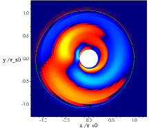
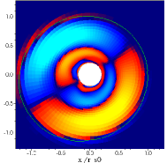
Figure 5.— Evolution of the azimuthal velocity in the equatorial plane at $t\simeq 30{t_{\rm ff0}}$ for models R2_L11f (left) and R2_L11h (right), which are closer in size to stalled supernova shocks, but have several unstable $\ell=1$ overtones. When the fundamental is excited (left), an irregular spiral is obtained, whereas an excitation of the first overtone yields an oblique sloshing mode at the fundamental frequency (right). The color scale is the same as in Figure 4.

As a mode grows in amplitude, the pressure perturbation shown in Figure 1k develops into a protuberance that rotates with the oscillation period of the instability. Eventually a shock forms at the interface where the two streams move towards each other, resulting in a triple point at the shock (Blondin & Shaw 2007). Figure 6 shows the morphology of the shock right before this triple point forms, for models R5_L11P2, R6_L21P2, and R6_L22P2.

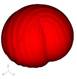
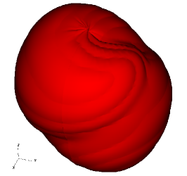
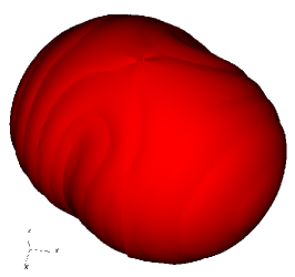
Figure 6.— Isobaric surfaces ($p=0.1\rho_{1}{v_{\rm ff0}^{2}}$), showing the morphology of the shock in the transition to the nonlinear regime for models R5_L11P2 at $t=46.5{t_{\rm ff0}}$ (left), R6_L21P2 at $t=57{t_{\rm ff0}}$ (middle), and R6_L22P2 at $t=52.5{t_{\rm ff0}}$ (right). In all cases, the ratio $r_{*}/{r_{\rm s0}}$ is chosen so that only the fundamental mode is unstable, for each $\ell$. The meridional line at $y=0$ is an artifact of the plotting tool, while the irregularity at the north pole is due to the numerical instability described in section 2.3. In all cases, the shock deformations grow in amplitude and rotate counterclockwise. An animated version of this Figure is available in the online version of the article.

The initial phase of exponential growth of isolated modes is followed by nonlinear mode coupling and saturation. Figures 7a and 7b show the spherical harmonic coefficients

$$a_{\ell,m}(t)=\int{\mathrm{d}}\Omega\,Y_{\ell}^{m}\,R_{s}(\theta,\phi,t),$$ (13)

where $R_{s}(\theta,\phi,t)$ is an isobaric surface tracing the shock, as a function of time for models R5_L11P2c and R5_L11P4. In both cases, the primary sloshing mode combination remains isolated in the linear phase, along with a non-oscillatory increase in the $\ell=2$, $m=0$ mode due to the increasing oblateness of the shock, likely caused by the redistribution of angular momentum (§4.2). Other modes are excited only after the primary mode reaches nonlinear amplitudes. Interestingly, the first modes to couple are $Y_{2}^{\pm 2}$, which achieve amplitudes about 50% lower than the primary mode. The axisymmetric $\ell=1$ mode together with $\ell=2$, $m=\{0,\pm 1\}$ modes couple much later, and do not reach as large an amplitude as $m=2$. We do not show $\ell=3$ results to keep Figure 7 legible, but a similar trend is observed in that $Y_{3}^{\pm 3}$ couple first and reach the largest amplitudes of all $\ell=3$ modes. This sequence of mode coupling differs from that found by Iwakami et al. (2008a), who witnessed the $\ell=2$, $m=0,\pm 1$ modes to couple first and reach the largest amplitude behind $\ell=1$. However, their non-axisymmetric perturbation excites the real spherical harmonics $Y_{1}^{0}$ and $Y_{1}^{1}$ in phase, hence it is not surprising that the mode coupling sequence differs.

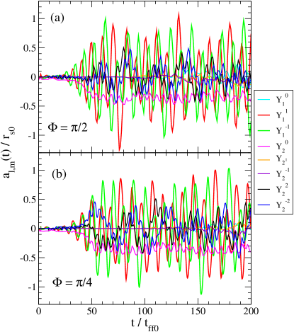
Figure 7.— Real spherical harmonic coefficients of the shock (traced by an isobaric surface) as a function of time, for models R5_L11P2c (top) and R5_L11P4 (bottom). The linear phase lasts approximately until the $\ell=1$ displacement is $\sim 10\%$ of the postshock cavity, or $t\simeq 30{t_{\rm ff0}}$. Full saturation is reached around $t=60{t_{\rm ff0}}$. Note that the $Y_{1}^{\pm 1}$ coefficients do not fall into the same envelope in the linear phase, indicating that they were not excited with the same amplitude.

To track how the relative phase in the primary spiral mode evolves going into the nonlinear phase, we compute a normalized cross-correlation between the spherical harmonic coefficients of the corresponding sloshing modes:

$$\mathrm{CC}[a_{1,1},a_{1,-1}](\Delta t)=$$

$$\frac{\int\,dt\,\left[a_{1,1}(t)-\bar{a}_{1,1}\right]\left[a_{1,-1}(t+\Delta t)-\bar{a}_{1,-1}\right]}{\left(\int dt\left[a_{1,1}(t)-\bar{a}_{1,1}\right]^{2}\right)^{1/2}\left(\int\,dt\left[a_{1,-1}(t)-\bar{a}_{1,-1}\right]^{2}\right)^{1/2}},$$ (14)

where $\bar{a}_{\ell,m}$ is the time average of $a_{\ell,m}$ and the integrals are performed over the same time interval $[t_{\rm{min}},t_{\rm{max}}]$. Figure 8 shows the results of applying equation (4.1) to the linear and nonlinear phase of modes R5_L11P2c, R5_L11P4, and R5_L11P4, which differ only in the initial relative phase of the perturbation. In the linear regime, the cross-correlation has an initial peak at a time delay $\Delta t_{1}=\Phi/\omega_{osc}$. As this amounts to shifting the second sloshing mode back into the first, equation (4.1) yields values near unity. Subsequent peaks arise at $\Delta t_{n}=(\Phi+n\pi)/\omega_{osc}$, ($n=1,2,...$), with an amplitude $(-1)^{n}\exp(-n\pi\omega_{\rm grow}/\omega_{\rm osc})$, i.e., each half period down in magnitude by the inverse exponential growth rate, with alternating sign. When equation (4.1) is applied to the fully saturated nonlinear phase, the first peak shifts to a larger value of $\Delta t$ relative to the linear phase, with no significant change in amplitude between subsequent peaks. Furthermore, the three nonlinear cross-correlations are nearly identical, with a period $\simeq 12{t_{\rm ff0}}$ and a time delay $\simeq 2.5{t_{\rm ff0}}$, corresponding to a phase shift $\simeq 2\pi/5$. This suggests that the development of spiral modes in the fully saturated stage is independent of the initial conditions, for any non-zero initial relative phase between sloshing modes. As mentioned in §3, a larger class of initial perturbations can therefore result in spiral modes, not just those tuned to a relative phase of $\pi/2$.

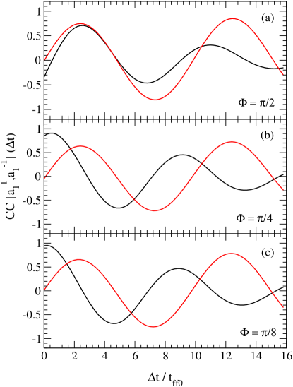
Figure 8.— Normalized cross-correlation (eq. [4.1]) applied to models R5_L11P2c (top), R5_L11P4 (middle), and R5_L11P8 (bottom). Shown is the linear and weakly nonlinear phase (black), covering the time interval $t\in[24,50]{t_{\rm ff0}}$, and the fully saturated phase (red), over $t\in[100,200]{t_{\rm ff0}}$ (see Figure 7). The ratio of consecutive peaks in the linear phase is approximately $\exp{(\pi\omega_{\rm grow}/\omega_{\rm osc})}$, or the fraction of an e-folding corresponding to one-half of an oscillation period. The initial condition is reflected in the cross-correlation taken over the linear phase. However, the time-delay between sloshing modes in the nonlinear phase is almost independent of initial conditions.

We have also performed a simulation in which, instead of using overdense shells, we impose random cell-to-cell pressure perturbations below the shock (R5_RAN). For this, we employ the setup with $r_{*}/{r_{\rm s0}}=0.5$, for which only the fundamental $\ell=1$ mode is unstable (and the most unstable for all $\ell$). Figure 9a shows the corresponding spherical harmonic coefficients as a function of time. Initially, a sloshing mode along the $z$-axis is triggered due to the form of the grid. However, as this mode reaches the nonlinear phase, a sloshing mode along the $y$ axis emerges out-of-phase, and then another along the $x$ axis follows. Figure 9b shows the normalized cross-correlation in the nonlinear phase, for the three different $\ell=1$ mode combinations over the time interval $t\in[200,300]{t_{\rm ff0}}$, showing that all of them are out-of phase. Note that the phase delay between $Y_{1}^{1}$ and $Y_{1}^{-1}$ is nearly the same as that in Figure 8 (modulo half a period), even though $Y_{1}^{1}$ is still growing in amplitude. The resulting angular momentum redistribution is discussed in §4.2.

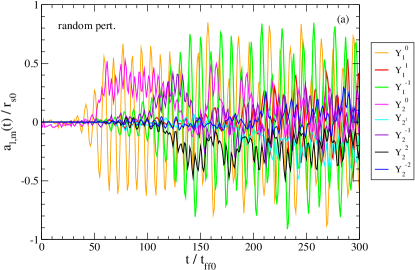
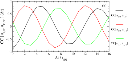
Figure 9.— Top: spherical harmonic coefficients for model R5_RAN. The initial bias towards axisymmetric ($Y_{1}^{0}$ and $Y_{2}^{0}$) perturbations is due to the form of the grid (more cells closer to the poles). Non-axisymmetric modes do indeed grow out of numerical noise, as expected. Bottom: normalized cross-correlation (eq. [4.1]) applied over the time interval $t\in[200,300]{t_{\rm ff0}}$ to the $\ell=1$ modes pairwise. All three of them are out-of-phase with each other in the nonlinear phase, leading to angular momentum redistribution (Figure 16).

To close this subsection, we address the effects of dimensionality and resolution on the saturation amplitude. Table 2 shows the rms fluctuation of the $a_{1,1}$ spherical harmonic coefficient around its mean for various models. There does not appear to be a systematic difference between the saturation amplitude in 2D and 3D at this resolution and with this numerical method. The changes due to the presence of the cutout around the polar axis or a resolution doubling are of the same magnitude, $\sim 10\%$. Similarly, whether the sloshing mode is isolated or part of a spiral mode seems to make a small difference, which is a weak function of the relative phase between modes. In the context of parasitic instabilities (Guilet et al. 2010), this indicates that either (i) the resolution is still too low to expose the different growth rates of parasites in 2D and 3D, or (ii) given the structure of these modes, the difference in the growth rates does not translate in sizable differences in the saturation amplitudes.

Table 2Saturation Amplitude of $Y_{1}^{1}$ mode

Model	Dimensionality	Resolution	$\Delta a_{1,1}\tablenotemark{b}$
r5_L1_LR	2D	$\phantom{1}56\times 48$	0.505
r5_L1_LRc	2D	$\phantom{1}56\times 48$c	0.424
r5_L1_HR	2D	$112\times 96$	0.412
r5_L1_HRc	2D	$112\times 96$c	0.454
R5_L11x	3D	$\phantom{1}56\times 48\times 96$c	0.473
R5_L11P2	3D	$\phantom{1}56\times 48\times 96$	0.505
R5_L11P2c	3D	$\phantom{1}56\times 48\times 96$c	0.499
R5_L11P4	3D	$\phantom{1}56\times 48\times 96$c	0.504
R5_L11P8	3D	$\phantom{1}56\times 48\times 96$c	0.481
R5_L11_HR	3D	$112\times 96\times 192$c	0.525

4.2. Angular Momentum Redistribution

Given that the background accretion flow has not net angular momentum, any net spin-up of the protoneutron star via accreted matter involves the separation of the postshock flow into regions with angular momentum of opposite sign (e.g., Blondin & Shaw 2007). In what follows, we explore how the linear and nonlinear phases of spiral modes mediate this angular momentum redistribution, and quantify the magnitude of the effect. To ease comparison with other studies, we express angular momenta in units of $\dot{M}{r_{\rm s0}}^{2}$, which amounts to dividing our results by $4\pi$ within the dimensionless unit system described in §2.1.

4.2.1 Linear Phase

Figure 10 shows the z-component of the angular momentum density integrated over a spherical surface at radius $r$

$$l_{z}(r)=r^{2}\int\,{\mathrm{d}}\Omega\,\rho\,r\sin\theta\,v_{\phi},$$ (15)

for model R5_L11_HR at various times during the linear phase. The upper panel shows times covering a full oscillation cycle, and the bottom shows curves rescaled by a factor $\exp{[-2\omega_{\rm grow}(t-t_{0})]}$ over a longer timescale, with $\omega_{\rm grow}$ the growth rate measured from the spherical harmonic coefficients. We thus infer that, in the linear phase, (i) a spiral mode has a characteristic angular momentum density profile which separates the flow into two counter-rotating regions, (ii) this profile is non-oscillatory, and (iii) it grows in amplitude at nearly twice the growth rate of the mode. The latter is consistent with the fact that $l_{z}(r)$ is a second-order quantity, as the zeroth- and first-order components of equation (15) vanish. To lowest order in $\Delta\xi/{r_{\rm s0}}$, it is made up of products of the form $\Delta\rho^{(1)}\Delta v_{\phi}^{(1)}$ and $\rho^{(0)}\Delta v_{\phi}^{(2)}$, where the superscripts in parentheses indicate explicitly the order of the perturbation.

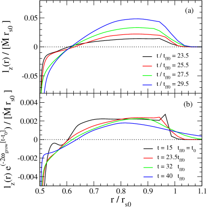
Figure 10.— Z-component of the angular momentum density integrated over a spherical surface $l_{z}(r)$ (eq. [15]) as a function of time for model R5_L11_HR. Top: Values at four times covering an entire $a_{1,1}$ oscillation period, showing that $l_{z}(r)$ is non-oscillatory. Bottom: values at a few times where the $Y_{1}^{1}$ mode is at phase zero, scaled by the square of the mode amplification factor relative to $t_{0}=15{t_{\rm ff0}}$, $\exp(-2\omega_{\rm grow}[t-t_{0}])$, showing that $l_{z}(r)$ grows at nearly twice the growth rate of the primary linear spiral mode.

We can separate out equation (15) into components

$$l_{z}(r) = l^{(0)(2)}+l^{(1)(1)}+{\rm O(3)}$$ (16)

$$l^{(0)(2)} = r^{3}\int\,{\mathrm{d}}\Omega\,\rho^{(0)}\,\sin\theta\Delta v_{\phi}^{(2)}$$ (17)

$$l^{(1)(1)} = r^{3}\int\,{\mathrm{d}}\Omega\,\Delta\rho^{(1)}\,\sin\theta\Delta v_{\phi}^{(1)}$$ (18)

where O(3) denotes higher order terms. Due to the fact that $\rho^{(0)}$ is spherically symmetric, only the $\ell=0$ component of $\sin\theta\,\Delta v_{\phi}^{(2)}$ survives:

$$\left[\sin\theta\Delta v_{\phi}^{(2)}\right]_{0,0}=\int\,{\mathrm{d}}\Omega\,Y_{0}^{0}\,\sin\theta\,v_{\phi}-{\rm O(3)}.$$ (19)

The first order components are the real parts of the complex perturbations

$$\Delta\rho^{(1)} = \frac{1}{2}\sum_{\ell,m}\left[\delta\tilde{\rho}_{\ell,m}\Upsilon_{\ell}^{m}e^{-i\omega_{\ell,m}t}+\delta\tilde{\rho}^{*}_{\ell,m}\Upsilon_{\ell}^{m*}e^{i\omega^{*}_{\ell,m}t}\right]$$ (20)

$$\sin\theta\Delta v_{\phi}^{(1)} = \frac{i}{2}\sum_{\ell,m}m\left[\delta\tilde{v}_{\Omega,\ell,m}\Upsilon_{\ell}^{m}e^{-i\omega_{\ell,m}t}\right.$$ (21)

$$\qquad\qquad-\left.\delta\tilde{v}^{*}_{\Omega\ell,m}\Upsilon_{\ell}^{m*}e^{i\omega^{*}_{\ell,m}t}\right],$$

where $\Upsilon_{\ell}^{m}$ denotes the usual complex spherical harmonics, and the star stands for complex conjugation. Integrating over angles yields

$$l^{(1)(1)}=r^{3}\sum_{\ell,m}m\, e^{2{\rm Im}(\omega_{\ell,m})t}\,\left[{\rm Im}(\delta\tilde{\rho}_{\ell,m}){\rm Re}(\delta\tilde{v}_{\Omega,\ell,m})\right.$$ (22)

$$\left.-{\rm Re}(\delta\tilde{\rho}_{\ell,m}){\rm Im}(\delta\tilde{v}_{\Omega,\ell,m})\right]+{\rm O(3)}.$$

Figure 11 shows $l_{z}(r)$ at time $t=23.5{t_{\rm ff0}}$ for model R5_L11_HR, where the $Y_{1}^{1}+iY_{1}^{-1}$ mode is at phase zero (cf. Figure 7). Also shown are $l^{(0)(2)}$, with both $\rho^{(0)}$ and $\sin\theta\,\Delta v_{\phi}^{(2)}$ obtained by projection of the corresponding fields fields onto $Y_{0}^{0}$, and the $\ell=1$, $m=1$ component of $l^{(1)(1)}$. For the latter, the real part of the complex amplitude at phase zero is the projection onto $Y_{1}^{1}$, while the imaginary part is minus the $Y_{1}^{-1}$ component. Most of the angular momentum density comes from $l^{(0)(2)}$, with $l^{(1)(1)}$ being a $\sim 10\%$ correction. Together, these terms account for almost all of $l_{z}(r)$, in agreement with the fact that modes with $\ell\geq 2$, $m\neq 0$ have a negligible amplitude in the linear phase.

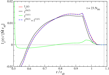
Figure 11.— Angular momentum density integrated over a spherical surface for model R5_L11_HR (red line, eq. [15]) as a function of radius, evaluated at $t=23.5{t_{\rm ff0}}$, where the spiral mode is at phase zero. Also shown are the dominant second order components $l^{(0)(2)}$ and $l^{(1)(1)}$ (defined in eqns. [16]-[18], black and green lines, respectively), where the latter is evaluated for the $\ell=1$, $m=1$ mode only (eq. [22]), and their sum (blue dashed lines). The vertical dotted line shows the average shock radius.

For comparison, figures 12a and b show the $Y_{1}^{\pm 1}$ components of the density and azimuthal velocity fields as a function of radius at $t=23.5{t_{\rm ff0}}$, for model R5_L11_HR, along with the eigenmodes from linear stability analysis normalized by the value of their respective spherical harmonic coefficients. Reasonable agreement is found between both approaches. Thus, most of $l^{(1)(1)}$ can be accounted for by linear theory. Figure 12c shows $[\sin\theta\,v_{\phi}^{(2)}]_{0,0}$ (eq. [19]). Note that the amplitude is $\sim 10$ times smaller than the first order $\ell=1$ components in Figure 12a.

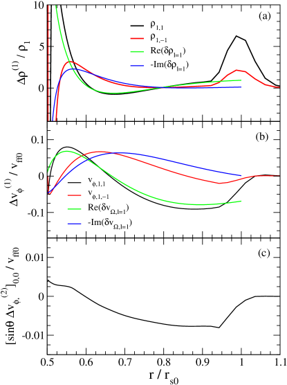
Figure 12.— Top: $\ell=1$, $m=\pm 1$ components of the density at time $t=23.5{t_{\rm ff0}}$ for model R5_L11_HR (black and red curves). Also shown are the corresponding values predicted by linear stability theory for a relative phase $\Phi=\pi/2$, with $Y_{1}^{1}$ at zero phase. The amplitude of the eigenfunctions has been normalized by the value of the shock spherical harmonic coefficients. Middle: same as top, but now for the azimuthal velocity (see Appendix A for the definition of $\delta v_{\Omega}$). The reasonable agreement with eigenfunctions means that $l^{(1)(1)}$ is mostly accounted for by linear theory. Bottom: The projection of the azimuthal velocity onto $Y_{0}^{0}$, which is second order (eq. [19]). Note that its amplitude is about 10 times smaller than the first-order $\ell=1$ perturbations in panel (b).

The angular momentum redistribution is a smooth process, mediated by exponential amplification. Thus, the formation of a triple point at the shock is not the main agent behind the the spin-up of the inner region, as we have shown that angular momentum redistribution begins as soon as linear modes are excited. The triple point may, however, be related to the saturation of the primary mode, setting the magnitude of the angular momentum redistribution.

A key element for a predictive theory of the spin-up due to exponentially growing spiral modes involves calculation of the second order velocity perturbation $\sin\theta\,v_{\phi}^{(2)}$, since $l^{(0)(2)}$ dominates the spin-up. We surmise that this would require repeating the steps followed for linear perturbations (A.1), but now expanding to second order in $\Delta\xi/{r_{\rm s0}}$. Combining this result with a criterion for the saturation of the SASI (such as that from Guilet et al. 2010) would allow estimation of the maximum angular momentum redistribution achievable by this means.

4.2.2 Nonlinear Phase and Total Spin-Up

We focus first on the high resolution $\ell=1$ model, R5_L11_HR, and then present results for other parameter combinations (Table 1). Figure 13 shows the evolution of the three components of the enclosed angular momentum

$$L_{i}(r)=\int_{r_{*}}^{r}\,l_{i}(s)\,{\mathrm{d}}s\,\qquad(i=x,y,z)$$ (23)

evaluated at $r=0.6{r_{\rm s0}}$, corresponding to the approximate radius at which $l_{z}(r)$ changes sign (see Figure 10). Two clear phases can be distinguished. First, from $t=0$ to $50{t_{\rm ff0}}$, $L_{z}$ grows exponentially due to the effects discussed in §4.2.1. Once other modes start to grow in amplitude, the torque becomes oscillatory and saturates together with the primary mode. Once full saturation has been reached, the transverse components $L_{x}$ and $L_{y}$ increase in magnitude and fluctuate stochastically around zero. The subsequent evolution in this fully saturated stage depends somewhat on the resolution employed. Model R5_L11_HR seems to remain in a quasi steady-state until the end of the integration at $t=180{t_{\rm ff0}}$, while model R5_L11P2c shows large amplitude and long period oscillations in $L_{z}$, and a secular increase in the magnitude of $L_{x}$ and $L_{y}$ at late times.

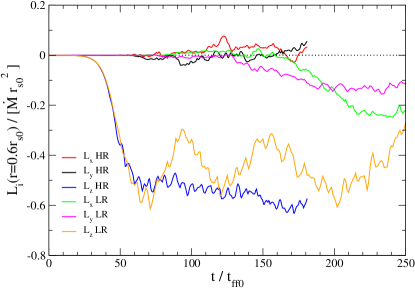
Figure 13.— Evolution of the three cartesian components of the enclosed angular momentum (eq. [23]) evaluated at $r=0.6{r_{\rm s0}}$, where $l_{z}(r)$ changes sign, for $\ell=1$, $m=\pm 1$ spiral modes at different resolution. Shown are $L_{x}$, $L_{y}$ and $L_{z}$ for model R5_L11_HR (red, black, and blue curves, respectively) and R5_L11P2c (green, magenta, and orange curves, respectively). The bulk of the angular momentum redistribution occurs during the exponentially growing phase, and the saturation value is a weak function of resolution. The subsequent evolution shows larger departures. Model R5_L11_HR is only evolved until $t=180{t_{\rm ff0}}$.

Figure 14 shows how the angular momentum redistribution depends on the polar and azimuthal indices of the primary spiral mode, as well as on the relative phase with which it is excited. In this case, the ratio $r_{*}/{r_{\rm s0}}$ is chosen so that only the fundamental mode is unstable for either $\ell=1$ or $\ell=2$, hence the primary spiral mode grows isolated in the linear phase. The top panel focuses on the low resolution runs that excite the $\ell=1$, $m=\pm 1$ modes (R5_L11P2c, R5_L11P4, and R5_L11P8). The maximum spin-up due to the primary spiral mode (along $L_{z}$) is weakly dependent on the initial relative phase, and has a magnitude $\sim 0.6\dot{M}{r_{\rm s0}}^{2}$. However, the time-delay required to achieve this maximum can differ by a factor of two. The transverse components ($L_{x}$ and $L_{y}$) do not show a significant difference, aside from the secular growth in the case $\Phi=\pi/2$, which is likely due to resolution effects (Figure 13). Figure 14b focuses on the $\ell=2$, $m=\pm 1$ modes, which still impart a spin-up along the z-axis despite having vanishing azimuthal velocity at the equator. Note however that the magnitude of the spin-up is much smaller than $\ell=1$ spiral modes. The magnitude of the transverse components at late times for $\Phi=\pi/2$ are to be taken with caution, again due to possible resolution effects. Finally, the $\ell=2$, $m=\pm 2$ modes show a behavior qualitatively similar to $\ell=1$, $m=\pm 1$, although the magnitude of the maximum angular momentum redistribution depends strongly on the relative phase. As with $\ell=2$, $m=\pm 1$, the maximum spin-up is much smaller in magnitude than $\ell=1$.

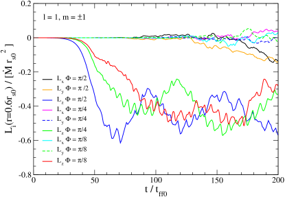
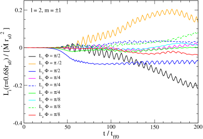
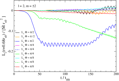
Figure 14.— Enclosed angular momentum components at fiducial radial positions for models where spiral modes with different spherical harmonic indices and relative phases are excited. Top: models R5_L11P2c, R5_L11P4, and R5_L11P8. The relative phase of the primary spiral mode is related to the time required to reach maximum spin-up. Middle: Same for models R6_L21P2c, R6_L21P4, and R6_L21P8. This time the angular momentum redistribution is more strongly dependent on initial relative phase. The radius $r=0.68{r_{\rm s0}}$ is equivalent in depth to that for runs with $r_{*}/{r_{\rm s0}}=0.5$. Bottom: Corresponding curves for models R6_L22P2c, R6_L22P4, and R6_L22P8. The behavior is somewhat similar to the modes with $\ell=1$, $m=\pm 1$, but the maximum spin-up does depend on initial phase. Note that the vertical scale is not the same.

The effects of changing the size of the postshock cavity ($r_{*}/{r_{\rm s0}}$) on the angular momentum redistribution are shown in Figure 15 for model R2_L11fc. Here, as in Figure 5a, the system has a size more similar to realistic core-collapse situations, but is such that many $\ell=1$ overtones are unstable. Still, a spin-up is observed, which is in fact larger than the case $r_{*}/{r_{\rm s0}}=0.5$. The secular growth of the spin-up, however, is to be taken with caution due to the low resolution of the model. The angular momentum redistribution following the phase of linear growth is still $\simeq 0.6\dot{M}{r_{\rm s0}}^{2}$. This initial peak, however, comes after a long time-delay of $130{t_{\rm ff0}}\simeq 400M_{1.3}^{-1/2}({r_{\rm s0}}/150~{}{\rm km})^{3/2}$ ms.

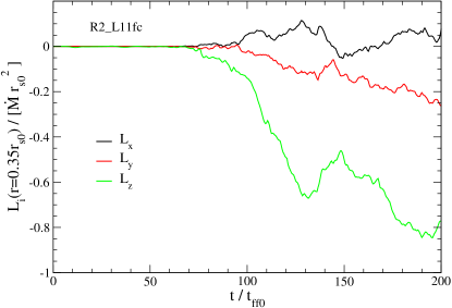
Figure 15.— Enclosed angular momentum within $r=0.35{r_{\rm s0}}$ for model R2_L11fc, for which $\ell=1$ has several unstable overtones (see Figure 5). The linear phase is qualitatively similar to that in model R5_L11P2c, but the maximum angular momentum is larger at longer times.

The effect of changing the initial perturbation is shown in Figure 16, which shows the angular momentum enclosed within $r=0.6{r_{\rm s0}}$ for model R5_RAN. The angular momentum amplification is directly related to the growth of spiral modes (compare with Figure 9). By the time integration stops, $Y_{1}^{1}$ is still growing, so $L_{y}$ may increase even more in magnitude. The fact that the spin-up along the z-axis is positive (in contrast to models R5_L11_HR and R5_L11P2c) is a consequence of the random initial relative phase between the corresponding sloshing modes. The spherical symmetry of the problem implies that changing the sign of $\Phi$ in equation (12) leads to angular momentum redistribution with the opposite sign.

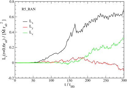
Figure 16.— Enclosed angular momentum within $r=0.6{r_{\rm s0}}$ for model R5_RAN (compare with Figure 9). The appearance of spiral modes induces a steady growth in the magnitude of the $L_{x}$ and $L_{z}$ components. Note that the model is evolved to later times.

The order-of-magnitude of the maximum angular momentum redistribution, $\dot{M}{r_{\rm s0}}^{2}$, can be understood if at saturation, the azimuthal velocity $v_{\phi}$ is close to the upstream velocity $v_{1}$. From linear theory (A.1), this follows for shock displacements of order unity, which is indeed the case for $\ell=1$ modes. Not so straightforward to explain is the size of the fluctuations in the fully saturated state, which involves interference between modes with different amplitudes and phases. The basic behavior of the spin-up during the exponential growth phase agrees with what was seen by Blondin & Shaw (2007) (their Figure 7), although they did not quantify their results in terms of fundamental physical quantities. Our results agree to within a factor of a few with those of Blondin & Mezzacappa (2007). They report typical spin-ups of $2.5\times 10^{47}$ at 250 ms (72${t_{\rm ff0}}$ for $M=1.2M_{\sun}$ and ${r_{\rm s0}}=230/1.5=153$ km, where 1.5 is our approximate average shock radius in units of ${r_{\rm s0}}$ and $230$ km their quoted shock position). At similar times, we find $0.6\dot{M}{r_{\rm s0}}^{2}\simeq 10^{47}(\dot{M}/0.36\,M_{\sun}~{}{\rm s}^{-1})({r_{\rm s0}}/153~{}{\rm km})^{2}$ g cm² s^-1. The differences could be caused by several factors: (i) their absorbing boundary condition with no cooling, which causes the shock to expand with time (e.g., Blondin et al. 2003), and (ii) resolution, which we have already shown to affect the long term behavior of the system.

Assuming that all of the angular momentum enclosed within the radius where $l_{z}(r)$ changes sign is accreted onto the neutron star, and that the latter has a moment of inertia $I_{\rm NS}=I_{45}\times 10^{45}$ g cm², one can write the minimum period due to spiral modes as

$$P\simeq 80\,I_{45}\dot{M}^{-1}_{0.3}\left(\frac{150~{}{\rm km}}{{r_{\rm s0}}}\right)^{2}\left(\frac{0.6}{f_{\rm amp}}\right)~{}{\rm ms},$$ (24)

where $f_{\rm amp}$ is the fraction of $\dot{M}{r_{\rm s0}}^{2}$ achieved during the phase of exponential growth. If no exponentially growing spiral mode takes place, one can still expect to achieve $f_{\rm amp}\lesssim 0.1$ from stochastic fluctuations, in which case the spin period $P\gtrsim 500$ ms. Figure 17 shows the evolution of the spin period for a few representative modes, taking into account the three components of the angular momentum, $P=2\pi I_{\rm NS}/\sqrt{L_{x}^{2}+L_{y}^{2}+L_{z}^{2}}$, with the $L_{i}$ measured at the radius at which $l_{z}(r)$ changes sign.

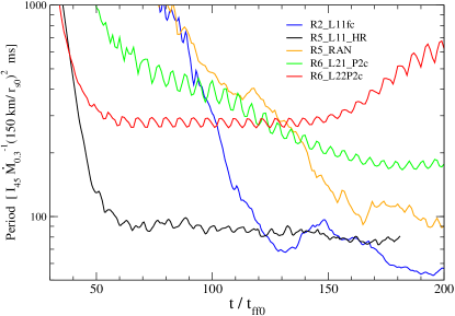
Figure 17.— Minimum neutron star spin periods, obtained by assuming that all of the angular momentum enclosed within the radius at which $l_{z}(r)$ changes sign is accreted onto a star of moment of inertia $I_{\rm NS}=10^{45}I_{45}$, for different models and as a function of time. All components of the angular momentum are included.

This simplistic picture is bound to change when more realistic physics is included. First, because it is not clear yet that spiral modes can easily develop in a convective gain region (e.g., Iwakami et al. 2008a), but also because both the neutrinosphere radius, the mass accretion rate, and the shock radius change as a function of time. The onset of explosion further complicates the picture, as the mass accretion is cut off and the postshock flow expands. Still, anisotropic cold and fast downflows piercing the convective region are expected to impart stochastic torques to the forming neutron star (Thompson 2000), an effect that we cannot capture with our current setup.

5. Summary and Discussion

In this paper we have studied the spiral modes of the SASI in the linear and nonlinear regime, when no rotation is imposed on the accretion flow, and when neutrino driven convection is suppressed. We have combined results from linear stability analysis and time-dependent simulations to understand the structure and evolution of these non-axisymmetric modes. Our main findings follow:

1. – Spiral modes are most easily understood as two or more sloshing modes out of phase. In the linear regime and in the absence of rotation, their three-dimensional structure can be obtained by linear superposition of known axisymmetric eigenfunctions. The parameters that determine a spiral mode are the number of sloshing modes involved, their relative phases, and amplitudes. Two modes of equal amplitude and relative phase equal to $\pm\pi/2$ is a limiting case of a more general class of non-axisymmetric mode.

2. – As long as the initial relative phase is not zero, spiral modes survive in the nonlinear phase. For the $\ell=1$, $m=\pm 1$ case, they seem to reach some type of equilibrium relative phase once all modes are excited in the fully saturated stage. This equilibrium phase does not seem to depend on the initial phase shift. Hence, the range of perturbations needed to excite spiral-like behavior leading to protoneutron star spin-up is broader than that needed to achieve spiral modes with a relative phase of $\pi/2$. The absolute sign of the angular momentum component in the inner and outer region depends on the sign of the initial relative phase.

3. – The angular momentum redistribution in the linear and weakly nonlinear phase of an isolated spiral mode is caused by the spatial dependence of the angular momentum density, which consists of at least two counterotating regions. This division occurs because the eigenmodes have at least one radial node in the transverse velocity profile (see, e.g., Figure 12b-c). The angular momentum density is non-oscillatory, and increases in magnitude at nearly twice the growth rate of the spiral mode. For $\ell=1$, we have found that the dominant term involves a second order perturbation to the azimuthal velocity, which couples to the background density. We see no apparent relation between the formation of the triple point at the shock and the angular momentum redistribution, other than a possible role in the saturation of the primary mode and hence a cutoff in the growth of the spin-up.

4. – The bulk of the angular momentum redistribution is achieved at the end of the phase of exponential growth. After $200$ dynamical times, our models achieve a maximum spin-up of at least $0.6\dot{M}{r_{\rm s0}}^{2}$ along the axis of the primary spiral mode, independent of the resolution employed, but restricted to $\ell=1$. Modes with $\ell=2$ also lead to spin-up along the primary axis, but with a smaller magnitude.

5. – In the fully saturated stage, where all modes are excited due to nonlinear coupling, all components of the angular momentum fluctuate with a characteristic magnitude $\lesssim\dot{M}{r_{\rm s0}}^{2}/10$. Resolution seems to be relevant for capturing the long-term evolution of the spin-up, which can display secular increases in magnitude at low resolution.

Blondin & Mezzacappa (2007) found that the development of spiral modes at late times is a robust feature of the flow, as many different types of perturbation resulted in a similar outcome when the accretion flow is non-rotating. Our results tend to confirm this picture. This was not the case in the simulations of Iwakami et al. (2009a), which however include neutrino heating and thus convection, fundamentally altering the flow dynamics relative to the simpler case with no heating. The fact that most progenitor models are likely to show some degree of rotation will always make excitation of a prograde spiral mode more likely, as its growth rate is larger (Yamasaki & Foglizzo 2008). Indeed, the development of SASI-like spiral modes has been observed in time dependent studies of accretion disks around a Kerr black hole (Nagakura & Yamada 2009)

Are overdense shells with large angular extent realistic? Two- and three-dimensional compressible simulations of carbon and oxygen shell burning in a $23M_{\sun}$ star find that density fluctuations of order $10\%$ are obtained due to internal waves excited in the stably stratified layers that lie in between convective shells (Meakin & Arnett 2006, 2007a, 2007b). These large amplitude fluctuations are due to the strong stratification, and are correlated over large angular scales (Meakin & Arnett 2007a). The oxygen-carbon interface lies too far out in radius to reach the stalled shock during the crucial few hundred milliseconds after bounce. But if a similar phenomenon were to occur above the Si shell, it would have a definite impact on the evolution of the stalled shock. Given that typical SASI periods are $\sim 30$ ms, all that is needed is a region of radial extent $\lesssim v_{\rm ff}/\omega_{\rm osc}\sim 200M_{1.3}^{1/2}r_{\rm 150}^{-1/2}$ km by the time it reaches the shock.

A different question is whether this coherent superposition of linear modes can take place in an environment where turbulent neutrino-driven convection already operates. The convective growth time in the gain region is a few ms (e.g., Fryer & Young 2007) compared to the several tens of ms required for the SASI to grow. A critical parameter determining the interplay between these two instabilities is the integral of the buoyancy frequency multiplied by the advection time over the gain region (Foglizzo et al. 2006). If this dimensionless parameter $\chi$ is less than 3, then infinitesimal perturbations do not have time to grow before they are advected out of the heating region, and a large amplitude perturbation is required to trigger convection. Using axisymmetric simulations with approximate neutrino transport and a realistic equation of state, Scheck et al. (2008) found that for weak neutrino heating, the SASI overturns can actually trigger convection. On the other hand, using parametric simulations, Fernández & Thompson (2009a) found that when $\chi>3$, convection grows rapidly and the vorticity distribution reaches its asymptotic value before the SASI achieves significant amplitudes. Two-dimensional convection is volume filling, as the vorticity accumulates on the largest spatial scales, hence large scale convective modes could be exciting dipolar SASI modes. The interplay between these two instabilities is not well understood at present, hence discussion of spiral modes in this context will have to wait for further work.

A few three-dimensional core-collapse simulations have been performed so far, some of these with highly dissipative numerical methods (Fryer & Young 2007; Iwakami et al. 2008a). These groups find that convection starts on smaller angular scales, with convective cells having roughly the size of the gain region (Fryer & Young 2007), or being mediated by high-entropy bubbles with a range of sizes (Iwakami et al. 2008a). In exploding simulations, as the shock expands, convective cells increase size and a global $\ell=1$ mode emerges (Fryer & Young 2007; Iwakami et al. 2008a). Persistent spiral modes do not seem to appear spontaneously, they need to be explicitly triggered (Iwakami et al. 2008a).

Very recently, Nordhaus et al. (2010) have reported three-dimensional, parametric core-collapse simulations using Riemann solvers and covering the whole sphere. Their results are in line with previous studies in that they do not witness the development of large scale shock oscillations in the stalled phase, or spiral modes with noticeable amplitudes. Similarly, Wongwathanarat et al. (2010) have presented full-sphere parametric explosions with a Riemann hydrodynamic solver, including the contraction of the protoneutron star and grey neutrino transport. Their conclusions are similar to that of Nordhaus et al. (2010) in that no coherent spiral modes are observed, with angular momenta saturating at a few times $10^{46}$ g cm² s^-1. Fryer & Young (2007) observe specific angular momenta $\lesssim 10^{13}$ cm² s^-1 imparted stochastically to the protoneutron star by anisotropic accretion. These values, and those of Wongwathanarat et al. (2010), are in agreement with the angular momentum fluctuations we observe in our fully saturated SASI, which on average have a magnitude $\sim 5\times 10^{12}(f_{\rm amp}/0.1)\dot{M}_{0.3}({r_{\rm s0}}/150~{}{\rm km})^{2}M^{-1}_{1.3}$ cm² s^-1.

Appendix A Calculation of Linear Eigenmodes

A.1. Background Flow and Perturbation Equations

The steady accretion flow below the shock is obtained by solving the time-independent Euler equations, using an ideal gas equation of state of adiabatic index $\gamma$ and the gravity of a point mass $M$,

$$\frac{\partial}{\partial r}(r^{2}\rho v_{r}) = 0$$ (A1)

$$v_{r}\frac{\partial v_{r}}{\partial r}+\frac{1}{\rho}\frac{\partial p}{\partial r}+\frac{GM}{r^{2}} = 0$$ (A2)

$$\frac{\partial p}{\partial r}-c_{s}^{2}\frac{\partial\rho}{\partial r} = (\gamma-1)\frac{\mathscr{L}}{v_{r}}.$$ (A3)

The boundary conditions at $r={r_{\rm s0}}$ are given by the Rankine-Hugoniot jump conditions (e.g., Landau & Lifshitz 1987). The upstream flow is adiabatic and has Mach number $\mathcal{M}_{1}$ at $r={r_{\rm s0}}$. For a given ratio $r_{*}/{r_{\rm s0}}$, the normalization of the cooling function is obtained by imposing $v_{r}(r_{*})=0$.

Foglizzo et al. (2007) introduce Eulerian perturbations of the form shown in equation (1). To obtain a compact formulation of the system, the following perturbation variables are employed

$$h = \frac{\delta v_{r}}{v_{r}}+\frac{\delta\rho}{\rho}$$ (A4)

$$f = v_{r}\delta v_{r}+\frac{\delta c^{2}}{\gamma-1}$$ (A5)

$$\delta S = \frac{1}{\gamma-1}\left(\frac{\delta p}{p}-\gamma\frac{\delta\rho}{\rho}\right)$$ (A6)

$$\delta K = r^{2}\mathbf{v}\cdot(\nabla\times\delta\mathbf{w})+\ell(\ell+1)\frac{p}{\rho}\delta S,$$ (A7)

corresponding to the perturbed mass flux, energy flux, entropy, and an entropy-vortex combination, respectively. The differential system for the radial profile of linear perturbations is obtained by perturbing the time-dependent fluid equations to first order, and rewriting the resulting equations in terms of (A4)-(A7), obtaining (Foglizzo et al. 2007)

$$\frac{\partial h}{\partial r} = \frac{i\delta K}{\omega r^{2}v_{r}}+\frac{i\omega}{v_{r}(1-\mathcal{M}^{2})}\left[\frac{\mu^{2}}{c^{2}}f-\mathcal{M}^{2}h-\delta S\right]$$ (A8)

$$\frac{\partial f}{\partial r} = \delta\left(\frac{\mathscr{L}}{\rho v_{r}}\right)+\frac{i\omega v_{r}}{(1-\mathcal{M}^{2})}\left[h-\frac{f}{c^{2}}+\left(\gamma-1+\frac{1}{\mathcal{M}^{2}}\right)\frac{\delta S}{\gamma}\right]$$ (A9)

$$\frac{\partial\delta S}{\partial r} = \frac{i\omega}{v_{r}}\delta S+\delta\left(\frac{\mathscr{L}}{pv_{r}}\right)$$ (A10)

$$\frac{\partial\delta K}{\partial r} = \frac{i\omega}{v_{r}}\delta K+\ell(\ell+1)\delta\left(\frac{\mathscr{L}}{\rho v_{r}}\right),$$ (A11)

where $\mu^{2}=1-(1-\mathcal{M}^{2})[\ell(\ell+1)c^{2}/r]/\omega^{2}$ and $\mathcal{M}$ is the Mach number. The shock boundary conditions for equations (A8)-(A11) are obtained from the perturbed shock jump conditions evaluated at the unperturbed shock position ${r_{\rm s0}}$ (Foglizzo et al. 2007),

$$h_{2} = \left(\frac{1}{v_{2}}-\frac{1}{v_{1}}\right)\Delta v$$ (A12)

$$f_{2} = \left(\frac{\mathscr{L}_{1}}{\rho_{1}v_{1}}-\frac{\mathscr{L}_{2}}{\rho_{2}v_{2}}\right)\Delta\xi+(v_{2}-v_{1})\Delta v$$ (A13)

$$\delta S_{2} = \frac{\rho}{p}\left[\frac{\mathscr{L}_{1}}{\rho_{1}v_{1}}-\frac{\mathscr{L}_{2}}{\rho_{2}v_{2}}-\left(\frac{GM}{{r_{\rm s0}}^{2}}-2\frac{v_{1}v_{2}}{{r_{\rm s0}}}\right)\left(1-\frac{v_{2}}{v_{1}}\right)\right]\Delta\xi$$ (A14)

$$-\frac{v_{1}}{p/\rho}\left(1-\frac{v_{2}}{v_{1}}\right)^{2}\Delta v$$

$$\delta K_{2} = \ell(\ell+1)\left[(v_{1}-v_{2})\Delta v+f_{2}\right],$$ (A15)

where $\Delta\xi$ is the shock displacement, $\Delta v=-i\omega\Delta\xi$ the shock velocity, and the subscripts $1$ and $2$ refer to quantities above and below the shock, respectively. The reflecting boundary condition at $r=r_{*}$ is

$$\delta v_{r}=\frac{v_{r}}{(1-\mathcal{M}^{2})}\left[h+\delta S-\frac{f}{c^{2}}\right]=0,$$ (A16)

resulting in a complex eigenvalue $\omega$.

A.2. Transverse Velocity Perturbation

The transverse components of the perturbed Euler equation are

$$-i\omega\,\delta v_{\theta}+\frac{v_{r}}{r}\frac{\partial\,\delta v_{r}}{\partial\theta}+v_{r}\,\delta w_{\phi}+\frac{1}{\rho\,r}\frac{\partial\delta p}{\partial\theta} = 0$$ (A17)

$$-i\omega\,\delta v_{\phi}+\frac{v_{r}}{r\,\sin\theta}\frac{\partial\,\delta v_{r}}{\partial\phi}-v_{r}\,\delta w_{\theta}+\frac{1}{\rho\,r\,\sin\theta}\frac{\partial\delta p}{\partial\phi} = 0,$$ (A18)

from which one can readily solve for $\delta v_{\theta}$ and $\delta v_{\phi}$ if the transverse components of the vorticity $\mathbf{w}$ are known. Note that, since $\delta v_{r}$ and $\delta p$ are proportional to $Y_{\ell}^{m}$ (§2.2), one has $\{\delta v_{\theta},\,\delta w_{\phi}\}\propto\partial Y_{\ell}^{m}/\partial\theta$, and $\{\delta v_{\phi},\,\delta w_{\theta}\}\propto\partial Y_{\ell}^{m}/(\sin\theta\,\partial\phi)$. Hence the only additional quantity required is the radial profile of the vorticity.

Taking the curl of the Euler equation yields

$$\frac{\partial\delta\mathbf{w}}{\partial t}-\nabla\times\left(\mathbf{v}\times\delta\mathbf{w}\right)-\frac{1}{\rho^{2}}\left(\nabla\rho\times\nabla p\right)=0.$$ (A19)

The inertial term can be expanded as

$$\nabla\times(\mathbf{v}\times\delta\mathbf{w})=v_{r}\left(\nabla_{\Omega}\cdot\delta\mathbf{w}_{\Omega}\right)\hat{r}-\frac{1}{r}\frac{\partial}{\partial r}\left(r\,v_{r}\,\delta\mathbf{w}_{\Omega}\right),$$ (A20)

where $\nabla_{\Omega}\cdot\delta\mathbf{w}_{\Omega}$ is the angular part of the divergence of the transverse vorticity, $\delta\mathbf{w}_{\Omega}=\delta w_{\theta}\,\hat{\theta}+\delta w_{\phi}\,\hat{\phi}$. Denoting by $\mathbf{B}$ the baroclinic term, one obtains

$$B_{r} = 0$$ (A21)

$$B_{\theta} = -\frac{1}{\rho_{0}^{2}}\left[\frac{1}{r\sin\theta}\frac{{\mathrm{d}}p_{0}}{{\mathrm{d}}r}\frac{\partial\,\delta\rho}{\partial\phi}-\frac{1}{r\sin\theta}\frac{{\mathrm{d}}\rho_{0}}{{\mathrm{d}}r}\frac{\partial\,\delta p}{\partial\phi}\right]$$ (A22)

$$B_{\phi} = -\frac{1}{\rho_{0}^{2}}\left[\frac{1}{r}\frac{{\mathrm{d}}\rho_{0}}{{\mathrm{d}}r}\frac{\partial\,\delta p}{\partial\theta}\phantom{\frac{1}{\sin\theta}}-\frac{1}{r}\frac{{\mathrm{d}}p_{0}}{{\mathrm{d}}r}\frac{\partial\,\delta\rho}{\partial\theta}\right].$$ (A23)

The equation governing the radial profile of the transverse vorticity is then

$$\frac{\partial\,\delta\mathbf{w}_{\Omega}}{\partial r}=\left[\frac{i\omega}{v_{r}}+\frac{1}{r}+\frac{1}{\rho_{0}}\frac{{\mathrm{d}}\rho_{0}}{{\mathrm{d}}r}\right]\delta\mathbf{w}_{\Omega}-\frac{1}{v_{r}}\mathbf{B}$$ (A24)

Once the radial profile of $\delta\mathbf{w}_{\Omega}$ is known, solving for $\delta w_{r}$ is straightforward, as no radial derivatives are involved.

The boundary condition at the shock for equation (A24) is obtained from equations (A17) and (A18), once the transverse velocity below the shock is known. Imposing $\hat{t}_{i}\cdot(\mathbf{v}_{2}+\delta\mathbf{v}_{2}-\mathbf{v}_{1})=0$ at the shock, where $\hat{t}_{i}$ are the tangent vectors

$$\hat{t}_{\theta} = \frac{1}{r}\frac{\partial\Delta\xi}{\partial\theta}\hat{r}+\hat{\theta}$$ (A25)

$$\hat{t}_{\phi} = \frac{1}{r\sin\theta}\frac{\partial\Delta\xi}{\partial\phi}\hat{r}+\hat{\phi},$$ (A26)

one obtains (e.g., Foglizzo et al. 2007)

$$\delta v_{\theta,2} = \frac{v_{r,1}-v_{r,2}}{{r_{\rm s0}}}\frac{\partial\Delta\xi}{\partial\theta}$$ (A27)

$$\delta v_{\phi,2} = \frac{v_{r,1}-v_{r,2}}{{r_{\rm s0}}\sin\theta}\frac{\partial\Delta\xi}{\partial\phi},$$ (A28)

where the subscripts $1$ and $2$ denote values upstream and downstream of the shock, respectively. We then obtain

$$\delta\tilde{w}_{r,2} = 0$$ (A29)

$$\delta\tilde{w}_{\theta,2} = -\frac{i\omega}{v_{r}}\delta\tilde{v}_{\phi,2}+\frac{1}{{r_{\rm s0}}}\delta\tilde{v}_{r,2}+\frac{1}{\rho{r_{\rm s0}}}\delta\tilde{p}_{2}$$ (A30)

$$\delta\tilde{w}_{\phi,2} = \frac{i\omega}{v_{r}}\delta\tilde{v}_{\theta,2}-\frac{1}{{r_{\rm s0}}}\delta\tilde{v}_{r,2}-\frac{1}{\rho{r_{\rm s0}}}\delta\tilde{p}_{2},$$ (A31)

where tildes denote the radial amplitude (eq. [1]). Given that $\delta\tilde{v}_{\theta,2}=\delta\tilde{v}_{\phi,2}$, it follows that $\delta\tilde{w}_{\phi,2}=-\delta\tilde{w}_{\theta,2}$. With this boundary condition, equations (A22), (A23), and (A24) imply that $\delta\tilde{w}_{\theta}(r)=-\delta\tilde{w}_{\phi}(r)$ for all $r$, and hence $\delta\tilde{v}_{\theta}(r)=\delta\tilde{v}_{\phi}(r)$ as well. For convenience, we adopt the notation

$$\delta\tilde{v}_{\Omega}(r)\equiv\delta\tilde{v}_{\theta}(r)=\delta\tilde{v}_{\phi}(r).$$ (A32)

Given the radial and angular form of the transverse velocity perturbations, one obtains $\delta w_{r}(r)=(\nabla\times\mathbf{v})_{r}=0$ everywhere.

Knowing that the transverse components of the vorticity have equal and opposite radial amplitudes, one can show from the definition of $\delta K$ (§2.2) that

$$\delta\tilde{w}_{\theta}=\frac{1}{rv_{r}}\left[\frac{\delta\tilde{K}}{\ell(\ell+1)}-\frac{p}{\rho}\delta\tilde{S}\right],$$ (A33)

that is, the amplitude of the vorticity can be directly obtained from the basic perturbation variables, without the need for solving equation (A24). We have nevertheless integrated this equation as a self-consistency check.

Appendix B Zeus-MP Implementation

B.1. Tensor Artificial Viscosity

Astrophysical hydrodynamic codes that employ finite difference algorithms to solve the Euler equations rely on artificial viscosity to broaden shocks over a few cells. This allows differencing of the flow variables without discontinuities, while obtaining the correct solutions to the jump conditions away from shocks. The standard practice is to use the prescription of VonNeumann & Richtmyer (1950), which only takes into account the spatial derivative of the velocity normal to the shock as an approximation to the divergence of the velocity field for determining compression. When curvilinear coordinates are used, however, this approach results in short wavelength oscillations behind the shock, and spurious heating of homologously contracting flows (e.g., Tscharnuter & Winkler 1979). To fix this, the artificial viscosity can be formulated as a coordinate-invariant tensor, which can correctly identify zones where the flow is compressed by becoming active only when $\nabla\cdot\mathbf{v}<0$ (Tscharnuter & Winkler 1979). Additional constraints on the functional form come from requiring that the artificial viscosity does not act on homologously contracting or shear flows (Tscharnuter & Winkler 1979; Stone & Norman 1992; Hayes et al. 2006).

In the context of core-collapse calculations, a tensor form of the artificial viscosity in Zeus-MP has previously been employed by Iwakami et al. (2008a), Iwakami et al. (2009a), and Iwakami et al. (2009b). They found that unless the tensor formulation is used, the carbuncle instability (Quirk 1994) appears at the poles of the shock (Iwakami et al. 2008b).

We have independently implemented a tensor artificial viscosity in Zeus-MP along the lines of Stone & Norman (1992) and Iwakami et al. (2008a), with some slight modifications. First, we use the volume difference instead of metric coefficient times coordinate difference (Stone & Norman 1992). This removes singularities at the polar axis whenever the factor $\sin\theta{\mathrm{d}}\theta$ appears in the denominator. Second, we have made use of the traceless nature of the artificial viscosity tensor to rewrite the $\theta$-component of its divergences as

$$\left(\nabla\cdot\mathbf{Q}\right)_{\,(2)} = \frac{1}{r\,\sin\theta}\frac{\partial}{\partial\theta}\left(\sin\theta\,Q_{22}\right)-\frac{Q_{33}}{r\sin\theta}\frac{\partial\sin\theta}{\partial\theta}$$ (B1)

$$= \frac{1}{r\,\sin^{2}\theta}\frac{\partial}{\partial\theta}\left(\sin^{2}{\theta}\,Q_{22}\right)+\frac{Q_{11}}{r\sin\theta}\frac{\partial\sin\theta}{\partial\theta},$$ (B2)

where the second expression is that used by Stone & Norman (1992) and Iwakami et al. (2008a). This allows to completely eliminate the metric coefficients of the denominator, by implementing the volume difference described above. The net effect is to reduce the noise in the $\theta$ velocity in the supersonic regions close to the z-axis, without making any significant difference at or below the shock.

When evolving our setup with this artificial viscosity prescription, the flow remains spherically symmetric and smooth for an indefinite time as long as there are no perturbations. If, on the other hand, the VonNeumann & Richtmyer (1950) prescription is used, the carbuncle instability indeed appears out of numerical noise within $\sim 10$ dynamical times, in agreement with Iwakami et al. (2008b).

However, when evolving sloshing SASI modes transverse to the z-axis, a runaway sawtooth instability of the $\phi$ component of the velocity develops around the axis whenever the amplitude (and thus the flow velocity) becomes large. This happens because the radial velocity at both sides of the axis is not the same, which in turn is caused by a wake generated by the reflecting axis. The reflection of the flow at the axis also compresses it, resulting in enhanced artificial viscosity dissipation at the axis, with irregular velocities. A similar phenomenon is observed in modes parallel to the z-axis, although the cause of this is not clear yet.

The cutout at the polar axis, described in the next subsection, suppresses the growth of this numerical instability to the point where meaningful results can be obtained. It does not, however, completely eliminate it. We proceed to the nonlinear phase based on the fact that the angular momentum contributed by regions around the shock and close to the polar axis is minor.

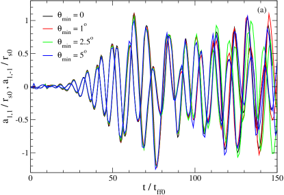
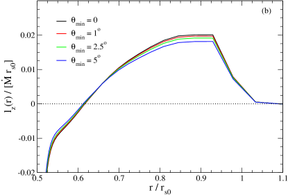
Figure 18.— Left: spherical harmonic coefficients for modes $Y_{1}^{1}$ and $Y_{1}^{-1}$ as a function of the half-opening angle $\theta_{\rm min}$ of the cutout around the polar axis. The cases $\theta_{\rm min}=0$ and $\theta_{\rm min}=5$ deg correspond to models R5_L11P2 and R5_L11P2c, respectively. Right: z-component of the angular momentum density integrated over a spherical surface (eq. [15]) at $t=24{t_{\rm ff0}}$ as a function of $\theta_{\rm min}$, for the same runs as the left panel.

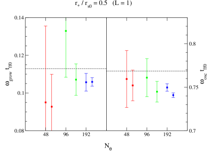
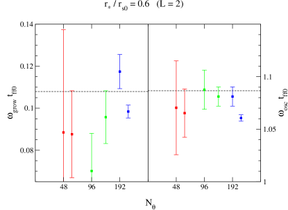
Figure 19.— Comparison of linear growth rates (left panels) and oscillation frequencies (right panels) from numerical simulations (squares) with values from linear stability analysis (dashed lines). The left plot shows results for $\ell=1$ ($r_{*}/{r_{\rm s0}}=0.5$) and the right $\ell=2$ ($r_{*}/{r_{\rm s0}}=0.6$). Different angular resolutions are color coded, with red, green, and blue corresponding to $N_{\theta}=48$, $96$ and $192$ cells over the whole range of polar angles, respectively. For each angular resolution, two points are shown, one with the baseline radial resolution (such that ${r_{\rm s0}}\Delta\theta=\Delta r$ at the shock) and another (to the right) with radial resolution doubled. At the resolution employed in this study, growth rates are reproduced within $20\%$, and oscillation frequencies within $10\%$ of the linear stability value.

B.2. Cutout at the Polar Axis

To investigate the reliability of results obtained with the axis cutout prescription described in §2.3, we performed two runs with half-opening angles $1$ and $2.5$ degrees, which fill the gap between models R5_L11P2 and R5_L11P2c. Figure 18a shows the spherical harmonic coefficients for modes $Y_{1}^{1}$ and $Y_{1}^{-1}$ as a function of time, for different values of the half-opening angle $\theta_{\rm min}$ of the cone that is removed from the grid around the polar axis. Aside from a $\sim 10\%$ reduction in the maximum amplitude, all curves follow nearly identical trajectories until $t\simeq 80{t_{\rm ff0}}$, where they start to diverge more noticeably. Panel (b) shows the angular momentum density integrated over a spherical surface at time $t=24{t_{\rm ff0}}$ (eq. [15], a low-resolution counterpart to Figure 11). Again, as the opening angle increases, results decrease by about $10\%$, consistent with the decrease in amplitude of shock oscillations. Other than that, the qualitative behavior is identical. We conclude that our resolution-independent results are reliable, with a quantitative uncertainty of at least $10\%$.

B.3. Linear Growth Rates

The eigenfrequencies obtained with the method described in Appendix A have been verified to high precision with time-dependent axisymmetric hydrodynamic simulations using the code FLASH2.5 (Fernández & Thompson 2009b). A basic test for the newly implemented setup is thus the reproduction of the linear SASI growth rates from linear stability analysis. This is a resolution-dependent requirement, hence convergence tests are needed. Figure 19 shows growth rates and oscillation frequencies as a function of angular and radial resolution, for axisymmetric simulations of $\ell=1$ and $\ell=2$ modes. The measurement method is the same as that described in Fernández & Thompson (2009b). With the baseline resolution employed in this study ($N_{\theta}=48$), growth rates are captured within $\sim 20\%$ and oscillation frequencies within $10\%$.

References

- Andersson et al. (2001) Andersson, N., Kokkotas, K. D., & Ferrari, V. 2001, International Journal of Modern Physics D, 10, 381
- Arfken & Weber (2005) Arfken, G. B., & Weber, H. J. 2005, Mathematical Methods for Physicists, sixth edn. (Amsterdam: Elsevier)
- Arzoumanian et al. (2002) Arzoumanian, Z., Chernoff, D. F., & Cordes, J. M. 2002, ApJ, 568, 289
- Binney & Tremaine (2008) Binney, J., & Tremaine, S. 2008, Galactic Dynamics, 2nd edn. (Princeton: Princeton Univ. Press)