Chemical abundances in the polar disk of NGC4650A: implications for cold accretion scenario

Abstract

The aim of the present study is to test whether the cold accretion of gas through a ”cosmic filament” (Macciò et al., 2006) is a possible formation scenario for the polar disk galaxy NGC 4650A. If polar disks form from cold accretion of gas, the abundances of the HII regions may be similar to those of very late-type spiral galaxies, regardless of the presence of a bright central stellar spheroid, with total luminosity of few $10^{9}L_{\odot}$.

We use deep long slit spectra obtained with the FORS2 spectrograph at the VLT in the optical and near-infrared wavelength ranges for the brightest HII regions in the disk polar disk of NGC 4650A. The strongest emission lines ([OII] $H_{\beta}$, [OIII], $H_{\alpha}$) were used to derived oxygen abundances, metallicities and the global star formation rates for the disk. The deep spectra available allowed us to measure the Oxygen abundances ($12+log(O/H)$) using the Empirical method based on intensities of the strongest emission lines, and the Direct method, based on the determination of the electron temperature from the detection of weak auroral lines, as the [OIII] at 4363 Å.

The Oxygen abundance measured for the polar disk is then compared with those measured for different galaxy types of similar total luminosities, and then compared against the predictions of different polar ring formation scenarios.

The average metallicity values for the polar disk in NGC 4650A is $Z=0.2Z_{\odot}$, and it is lower that the values measured for ordinary spirals of similar luminosity. Moreover the gradient of the metallicity is flat along the polar disk major axis, which implies none or negligible metal enrichment from the stars in the older central spheroid.

The low metallicity value in the polar disk NGC 4650A and the flat metallicity gradient are both consistent with a later infall of metal-poor gas, as expected in the cold accretion processes.

1 Introduction

The hierarchical, merger-dominated picture of galaxy formation is based on the Cold Dark Matter (CDM) model (Cole et al., 2000), which predicts that the observed galaxies and their dark halo (DH) were formed through a repeated merging process of small systems (De Lucia et al. 2006; Genel et al. 2008). In this framework, major and minor mergers of disky systems do play a major role in the formation of spheroid and elliptical galaxies (Naab et al. 2007; Bournaud et al. 2007), in all environments and from the Local Group to high-redshift universe (Conselice et al., 2003). The gas fraction is a key parameter in the physics of such gravitational interactions: if it is high enough, an extended and massive disk structure can survive (Springel & Hernquist 2005; Robertson & Bullock 2008). Galaxies can get their gas through several interacting processes, such as smooth accretion, stripping and accretion of primordial gas, which are equally important in the growth of galaxies. Recent theoretical works have argued that the accretion of external gas from the cosmic web filaments, with inclined angular momentum (Davé et al. 2001, Semelin & Combes 2005), might be the most realistic way by which galaxies get their gas. This process may also explain the build-up of high redshift disk galaxies (Kereš et al. 2005, Keres 2008, Brook et al. 2008, Dekel et al. 2009, Bournaud & Elmegreen 2009). The relative share of all gravitational interactions depends on the environments and it drives many morphological features observed in galaxies, such as bars and polar rings.

Galaxies with polar rings (PRGs) generally contain a central featureless stellar spheroid and an elongated structure, the “polar ring” (made up by gas, stars and dust), which orbits in a nearly perpendicular plane to the equatorial one of the central galaxy (Whitmore et al., 1990). The decoupling of the angular momentum of the polar structure and the central spheroid cannot be explained by the collapse of a single protogalactic cloud: thus a “second event” must have happened in the formation history of these systems. This is the reason why studying PRGs promise to yield detailed information about many of the processes at work during galaxy interactions and merging (Iodice et al. 2002, Iodice et al. 2002, Reshetnikov & Combes 1994, Reshetnikov et al. 2002, Bournaud & Combes 2003).

The debate on the origin of PRGs is still open and two main processes have been proposed i) a major dissipative merger or ii) gas accretion. In the merging scenario, the PRG results from a “polar” merger of two disk galaxies with unequal mass, (Bekki 1997; Bekki 1998; Bournaud et al. 2005): the morphology of the merger remnants depends on the merging initial orbital parameters and the initial mass ratio of the two galaxies. In the accretion scenario, the polar ring may form by a) the disruption of a dwarf companion galaxy orbitating around an early-type system, or by b) the tidal accretion of gas stripping from a disk galaxy outskirts, captured by an early-type galaxy on a parabolic encounter (Reshetnikov & Sotnikova 1997; Bournaud & Combes 2003; Hancock et al. 2009). In the latter case, the total amount of accreted gas by the early-type object is about $10\%$ of the gas in the disk donor galaxy, i.e. up to $10^{9}$ $M_{\odot}$. Both major merger and accretion scenarios are able to account for many observed PRGs morphologies and kinematics, such as the existence of both wide and narrow rings, helical rings and double rings (Whitmore et al., 1990).

Very recently, a new mechanism has been proposed for the formation of wide disk-like polar rings: a long-lived polar structure may form through cold gas accretion along a filament, extended for $\sim 1$ Mpc, into the virialized dark matter halo (Macciò et al., 2006). In this formation scenario, there is no limits to the mass of the accreted material, thus a very massive polar disk may develop either around a stellar disk or a spheroid. Brook et al. (2008), by using high-resolution cosmological simulations of galaxy formation, have confirmed and strengthened the formation scenario proposed by Macciò et al. (2006). In this case polar disk galaxies can be considered as extreme examples of angular momentum misalignment that occurs during the hierarchical structure formation. In the merging history, an inner disk formed first after the last major merger of two galaxies with a 1:1 mass ratio, then, due to the high gas fraction, the galaxy rapidly forms a new disk whose angular momentum depends on the merger orbital parameters. At later times, gas continues to be accreted along the disk which may be also in a plane perpendicular to the inner disk. The morphology and kinematics of one simulated object, in both simulations, are similar to those observed for NGC4650A: in particular, Brook et al. (2008) found that such formation mechanism can self-consistently explain both morphology and kinematics of central spheroid and polar structure, and all the observed features (like colors and colors gradient, longevity, spiral arms, HI content and distribution).

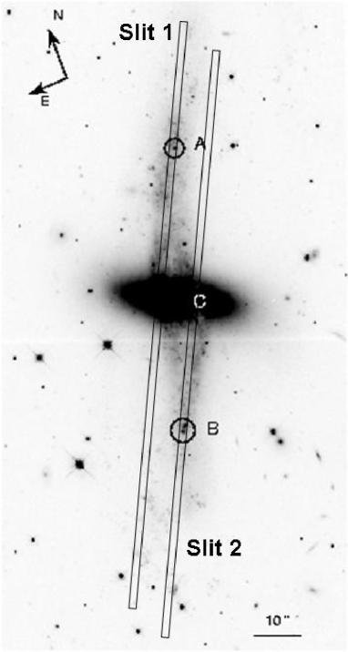
Figure 1: Optical image of NGC4650A with superimposed the slits used to acquire data analyzed in this work.

NGC 4650A is the prototype for PRGs (see Fig. 1). Its luminous components, inner spheroid and polar structure were studied in optical and near-infrared (NIR) photometry, spectroscopy, and in the radio emission, HI 21 cm line and continuum (Arnaboldi et al. 1997, Gallagher et al. 2002, Iodice et al. 2002, Swaters & Rubin 2003, Iodice et al. 2006).

The polar structure in NGC 4650A is a disk, very similar to that of late-type spirals or LSB galaxies, rather than a ring. The polar disk stars and dust can be reliably traced to $\sim 1.2$ kpc radius from the galaxy nucleus, and the surface brightness profiles have an exponential decrease (Iodice et al. 2002, Gallagher et al. 2002). Furthermore, the rotation curves measured from the emission and absorption line optical spectra are consistent with those of a disk in a differential rotation rather than that of a narrow ring (Swaters & Rubin, 2003). This is also confirmed by the HI 21 cm observations (Arnaboldi et al., 1997) which show that the gas is five times more extended than the luminous polar structure, with a position-velocity diagram very similar to those observed for edge-on disks. The polar disk is very massive, since the total HI mass is about $10^{10}M_{\odot}$, which added to the mass of stars, makes the mass in the polar disk comparable with the total mass in the central spheroid (Iodice et al., 2002). The morphology of the central spheroid resembles that of a low-luminosity early-type galaxy: the surface brightness profile is described by an exponential law, with a small exponential nucleus; its integrated optical vs. NIR colors are similar to those of an intermediate age stellar population (Iodice et al. 2002, Gallagher et al. 2002). New high resolution spectroscopy in NIR on its photometric axes suggests that this component is a nearly-exponential oblate spheroid supported by rotation (Iodice et al., 2006).

These new kinematic data, together with the previous studied, set important constraints on the possible formation mechanisms for NGC4650A.

Because of the extended and massive polar disk, with strong $H_{\alpha}$ emissions, NGC 4650A is the ideal candidate to measure the chemical abundances, metallicity and star formation rates (SFR) via spectroscopic measurements of line emissions along the major axis of the polar disk. The goal is to compare the derived values for the metallicity and SFR with those predicted by the different formation scenarios. As we shall detail in the following sections, if the polar structure forms by accretion of primordial cold gas from cosmic web filament, we expect the disk to have lower metallicities of the order of $Z\sim 1/10Z_{\odot}$ (Agertz et al., 2009) with respect to those of same-luminosity spiral disks.

We shall adopt for NGC4650A a distance of about 38 Mpc based on $H_{0}=75\ km\ s^{-1}\ Mpc^{-1}$ and an heliocentric radial velocity $V=2880\ km\ s^{-1}$, which implies that 1 arcsec = 0.18 kpc.

2 Observations and data reduction

Spectra were obtained with FORS2@UT1, on the ESO VLT, in service mode, during two observing runs: 078.B-0580 (on January 2007) and 079.B-0177 (on April 2007). FORS2 was equipped with the MIT CCD 910, with an angular resolution of $0.25^{\prime\prime}$ pixel^-1. The adopted slit is $1.6^{\prime\prime}$ wide and $6.8^{\prime}$ long. Spectra were acquired along the North and South side of the polar disk, at $P.A.=152^{\circ}$ (see Fig. 1), in order to include the most luminous HII regions in polar disk. The total integration time for each direction is 3 hours, during the 078.B-0580 run and 2.27 hours during 079.B-0177 run, respectively, with an average seeing of $1.2^{\prime\prime}$.

At the systemic velocity of NGC 4650A, to cover the red-shifted emission lines of the $[OII]\lambda 3727$, $[H_{\gamma}]\lambda 4340$, $[OIII]\lambda 4363$, $[OIII]\lambda\lambda 4959,5007$, $[H_{\beta}]\lambda 4861$, $[NII]\lambda 5755$ the grism GRIS-600B+22 was used in the $3300-6210$ Å wavelength range, with a dispersion of 50 Å/mm (0.75 Å/pix). In the near-infrared $5600-11000$Å wavelength range, the grism GRIS-200I+28 was used, with a dispersion of 162 Å/mm (2.43 Å/pix) to detect the fainter $[SII]\lambda\lambda 6717,6731$ and $[SIII]\lambda\lambda 9068,9532$ emission lines, with a $S/N\geq 20$ and the brighter $[H_{\alpha}]\lambda 6563$ emission line, with a $S/N>150$. In this wavelength range, where the sky background is much more variable and higher with respect to the optical domain, to avoid the saturation of the sky lines a larger number of scientific frames with short integration time (850 sec) were acquired.

The data reduction was carried out using the CCDRED package in the IRAF (Image Reduction and Analysis Facility) environment. The main strategy adopted for each data-set included dark subtraction, flat-fielding correction, sky subtraction and rejection of bad pixels. Wavelength calibration was achieved by means of comparison spectra of Ne-Ar lamps acquired for each observing night, using the IRAF TWODSPEC.LONGSLIT package. The sky spectrum was extracted at the outer edges of the slit, for $r\geq 40$ arcsec from the galaxy center, where the surface brightness is fainter than $24mag/arcsec^{2}$, and subtracted off each row of the two dimensional spectra by using the IRAF task BACKGROUND in the TWODSPEC.LONGSLIT package. On average, a sky subtraction better than $1\%$ was achieved. The sky-subtracted frames, both for North and South part of the polar disk, were co-added to a final median averaged 2D spectrum.

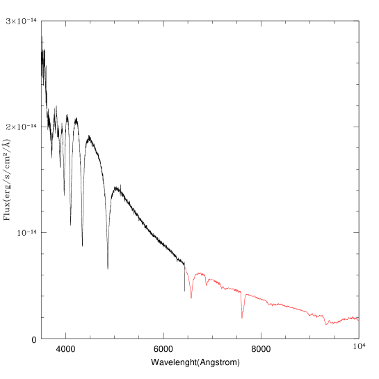
Figure 2: 1-D spectrum of the standard star LTT4816, used to flux-calibrate the spectra. The black line represent the spectrum of the star acquired in the blue wavelength range, while the red line is the same star acquired in the red range.

The final step of the data-processing is the flux calibration of each 2D spectra, by using observations of the standard star LTT4816 and the standard tasks in IRAF (STANDARD, SENSFUNC and CALIBRATE). The flux calibration is very important in the present study because we need to “align” two spectra, which cover different wavelength range and taken in different times. Thus, we checked and obtained that the calibrations for the spectra in both spectral range were consistent. Fig. 2 shows the 1D flux calibrated spectra of the spectrophotometric standard star used to calibrate the spectra in the whole range $3300-11000$ Å. To perform the flux calibration we extracted a 1-D spectrum of the standard star to find the calibration function; then we extracted a set of 1-D spectra of the galaxy summing up a number of lines corresponding to the slit width. Since the slit width was $1.3^{\prime\prime}$ and the scale of the instrument was $0.25^{\prime\prime}/pix$, we collapsed seven lines to obtain each 1-D spectrum. Finally we applied the flux calibration to this collection of spectra.

Furthermore, we compared our flux calibrated spectra with others acquired at the Siding Spring Observatory with the Double Beam Spectrograph (DBS) (Buttiglione et al., 2006). The DBS has a dichroic that slits the light in a red and a blue arm, therefore the flux calibration with standard stars can be done simultaneously for the red and the blue arms. We used these spectra to check for any difference in the flux calibrations, finding that our flux calibrated spectra, both of the template star and of the galaxy, turn out to be consistent with them.

The wavelength and flux-calibrated spectra are shown in Fig. 3 and 4. In the blue spectrum (top panel) are clearly visible a number of emission lines: $H_{\beta}$, $H_{\gamma}$, $[OII]\lambda 3727$ and $[OIII]\lambda\lambda 4959,5007$, while in the red one (bottom panel) we have $H_{\alpha}$ (blended with the $[NII]\lambda 6583$ line appearing in the red wing of $H_{\alpha}$), $[SII]\lambda\lambda 6717,6731$ and $[SIII]\lambda\lambda 9069,9532$. From a two-Gaussian fit to the combined emission, we estimate the line ratio $[NII]\lambda 6583/(H_{\alpha}+[NII]\lambda 6548\simeq 0.1$. For this reason the $H_{\alpha}$ flux is that measured as the total flux in the line reduced by the contribution of $[NII]\lambda 6583$. The observed emission lines and their uncorrected and reddening-corrected fluxes relative to $H_{\beta}$ are listed in Tab. 2 and Tab. 3.

Since ground-based near-infrared spectroscopy is affected by the strong and variable absorption features due to the Earth’s atmosphere, we accounted for this effect in our spectra, in which the telluric absorption bands are clearly visible around 7200, 8200 and 9300 Å. In order to perform this correction we used the ”telluric standard star” LTT4816, near both in time and air mass to the object, and the IRAF task TELLURIC; by fitting the continuum, telluric calibration spectra are shifted and scaled to best divide out telluric features from data spectra. The ratios of the uncorrected fluxes relative to those obtained applying the average telluric correction are the following: $[SII]\lambda 6717_{uncorrected}/[SII]\lambda 6717_{corrected}=[SII]\lambda 6731_{uncorrected}/[SII]\lambda 6731_{corrected}=1.7$ and $[SIII]\lambda 9069_{uncorrected}/[SIII]\lambda 9069_{corrected}=[SIII]\lambda 9532_{uncorrected}/[SIII]\lambda 9532_{corrected}=0.6$.

2.1 Measurement of emission-lines fluxes

The fluxes of the above mentioned emission lines were measured using the IRAF SPLOT routine, that provides an interactive facility to display and analyze spectra. The $H_{\beta}$ is evaluated for $r\geq 10$ arcsec, where only the emission line is present; for lower distances, i.e. where stars relative to the spheroid also contributes to the spectra, the $H_{\beta}$ is also in absorption. We evaluated flux and equivalent width by marking two continuum points around the line to be measured. The linear continuum is subtracted and the flux is determined by simply integrating the line intensity over the local fitted continuum. The errors on these quantities have been calculated, following Pérez-Montero & Díaz (2003), by the relation $\sigma_{1}=\sigma_{c}N^{1/2}[1+EW/(N\Delta)]^{1/2}$, were $\sigma_{1}$ is the error in the line flux, $\sigma_{c}$ is the standard deviation in a box near the measured line and represents the error in the continuum definition, N is the number of pixels used to measure the flux, EW is the equivalent width of the line and $\Delta$ is the wavelength dispersion in Å/pixel. The errors relative to each emission line fluxes are listed in Tab. 2 and Tab. 3.

2.2 Reddening correction

Reduced and flux calibrated spectra and the measured emission line intensities were corrected for the reddening, which account both for that intrinsic to the source and to the Milky Way. By comparing the intrinsic Balmer decrements, $H_{\alpha}/H_{\beta}=2.89$ and $H_{\gamma}/H_{\beta}=0.468$, predicted for large optical depth (case B) and a temperature of $10^{4}$ K, with the observed one, we derived the visual extinction $A(V)$ and the color excess $E(B-V)$, by adopting the mean extinction curve by Cardelli et al. (1989) $A(\lambda)/A(V)=a(x)+b(x)R_{V}$, where $R_{V}[\equiv\ A(V)/E(B-V)]=3.1$ and $x=1/\lambda$. In order to estimate reddening correction for all the observed emission lines, we used the complete extinction curve into three wavelengths regions (Cardelli et al. (1989)): infrared ($\lambda\geq 0.9\mu m$), optical/NIR ($0.9\mu m\geq\lambda\geq 0.3\mu m$) and ultraviolet ($0.125\mu m\geq\lambda\geq 0.10\mu m$), which are characterized by different relations of a(x) and b(x). All the emission lines in our spectra are in the optical/NIR range, except for the $[SIII]\lambda 9532$, that falls in the infrared range, so we used the average $R_{V}$-dependent extinction law derived for these intervals to perform the reddening correction.
We measured the fluxes of $H_{\beta}$, $H_{\gamma}$ and $H_{\alpha}$ lines at each distance from the galaxy center and for each spectra (North slit and South slit), than we derived the average observed Balmer decrements, which are the following:
$H_{\alpha}/H_{\beta}$ = $2.40\pm\ 0.01$
$H_{\gamma}/H_{\beta}$ = $0.41\pm\ 0.01$
while the color excess obtained by using these observed decrements are:
$[E(B-V)]_{H_{\alpha}/H_{\beta}}$ = $0.20\pm\ 0.004$
$[E(B-V)]_{H_{\gamma}/H_{\beta}}$ = $0.25\pm\ 0.012$.
Such values of E(B-V) are used to derive the extinction $A_{\lambda}$, through the Cardelli’s law; in particular, the $[E(B-V)]_{H_{\gamma}/H_{\beta}}$ and $[E(B-V)]_{H_{\alpha}/H_{\beta}}$ are used respectively for the reddening correction in optical and NIR wavelength range. The corrected fluxes are given by $F^{\lambda}_{int}/F^{H_{\beta}}_{int}=F^{\lambda}_{obs}/F^{H_{\beta}}_{obs}10^{0.4[A_{\lambda}-A_{H_{\beta}}]}$. Observed and reddening-corrected emission line fluxes are reported in Tab. 2 and Tab. 3.

3 Oxygen abundances determination

The main aim of the present work is to derive the chemical abundances in the polar disk of NGC4650A: in what follow we evaluate the oxygen abundances following the methods outlined in Pagel et al. (1979), Díaz & Pérez-Montero (2000) and Pilyugin (2001), referring to them as Empirical methods, and those introduced by Osterbrock (1989) and Allen (1984), or Direct methods.

The large dataset available (presented in Sec. 2) let us to investigate both the Empirical methods, based on the intensities of easily observable lines (Sec. 3.1), and the Direct method, based on the determination of the electron temperature, by measuring the intensities of the weak auroral lines (Sec. 3.2).
As described in details in the next sections, we have derived the oxygen abundance parameter $12+log(O/H)$ along the polar disk, by using both the Empirical and Direct methods.

3.1 Empirical oxygen and sulphur abundance measurements

The Empirical methods are based on the cooling properties of ionized nebulae which translate into a relation between emission-line intensities and oxygen abundance. Several abundance calibrators have been proposed based on different emission-line ratios: among the other, in this work we used $R_{23}$ (Pagel et al., 1979), $S_{23}$ (Díaz & Pérez-Montero, 2000) and the P-method (Pilyugin, 2001). The advantages of different calibrators have been discussed by several authors (Díaz & Pérez-Montero 2000, Kobulnicky & Zaritsky 1999, Kobulnicky & Kewley 2004, Pérez-Montero & Díaz 2005, Kewley & Ellison 2008, Hidalgo-Gámez & Ramírez-Fuentes 2009).

The method proposed by Pagel et al. (1979) is based on the variation of the strong oxygen lines with the oxygen abundance. Pagel et al. (1979) defined the ”oxygen abundance parameter” $R_{23}=([OII]\lambda 3727+[OIII]\lambda\lambda 4959+5007)/H_{\beta}$, which increase with the oxygen abundance for values lower than 20% of the solar one and then reverses his behavior, decreasing with increasing abundance, due to the efficiency of oxygen as a cooling agent that lead to a decreasing in the strength of the oxygen emission lines at higher metallicities. Three different regions can be identified in the trend of $R_{23}$ with the oxygen abundance (Pérez-Montero & Díaz, 2005): a lower branch ($12+log(O/H)<8.1$), in which $R_{23}$ increase with increasing abundance, an upper branch ($12+log(O/H)>8.4$), in which the trend is opposite, and a turnover region ($8.1<12+log(O/H)<8.4$). While the upper and lower branches can be fitted by regression lines, the turnover region seems to be the most troublesome, in fact object with the same value of $R_{23}$ can have very different oxygen abundances. The $R_{23}$ parameter is affected by two main problems: the two-valued nature of the calibration and the dependence on the degree of ionization of the nebula.

To break the degeneracy that affects the metallicity for values of $12+log(O/H)\geq 8.0$, Díaz & Pérez-Montero (2000) proposed an alternative calibrator, based on the intensity of sulphur lines: $S23=([SII]{\lambda}{\lambda}6717+6731+[SIII]{\lambda}{\lambda}9069+9532)/H_{\beta}$. The [SII] and [SIII] lines are analogous to the optical oxygen lines [OII] and [OIII], but the relation between the ”Sulphur abundance parameter $S_{23}$” and the oxygen abundance remain single valued up to solar metallicities (Díaz & Pérez-Montero 2000 and Pérez-Montero & Díaz 2005). Moreover, because of their longer wavelength, sulphur lines are less sensitive to the effective temperature and ionization parameter of the nebula, and almost independent of reddening, since the [SII] and [SIII] lines can be measured nearby hydrogen recombination lines. Díaz & Pérez-Montero (2000) have attempted a calibration of oxygen abundance through the sulphur abundance parameter, obtaining the following empirical relation:

$$12+log(O/H)=1.53logS_{23}+8.27$$ (1)

For the polar disk of NGC4650A, by using the emission line fluxes given in Tab. 2 and Tab. 3, we derived both $R_{23}$ and $S_{23}$ parameters, which are listed in Tab. 4. Since there are few measurements available for the Sulphur lines, we have obtained an average value of $S_{23}$ for the polar disk, by using the following telluric corrected fluxes ratios: $[SII]\lambda 6717/H_{\beta}=0.18$, $[SII]\lambda 6731/H_{\beta}=0.2$, $[SIII]\lambda 9069/H_{\beta}=0.43$ and $[SIII]\lambda 9532/H_{\beta}=0.25$, obtaining $logS_{23}=0.024\pm 0.030$. The average oxygen abundance, derived by adopting the Eq. 1, is the following: $12+log(O/H)_{S}=8.3\pm 0.2$.

Pilyugin (2001) realized that for fixed oxygen abundances the value of $X_{23}=logR_{23}$ varies with the excitation parameter $P=R_{3}/R_{23}$, where $R_{3}=OIII[4959+5007]/H_{\beta}$, and proposed that this latter parameter could be used in the oxygen abundance determination. This method, called ”P-method”, propose to use a more general relation of the type $O/H=f(P,R_{23})$, compared with the relation $O/H=f(R_{23})$ used in the $R_{23}$ method. The equation related to this method is the following

$$12+log(O/H)_{P}=\frac{R_{23}+54.2+59.45P+7.31P^{2}}{6.07+6.71P+0.371P^{2}+0.243R_{23}}$$ (2)

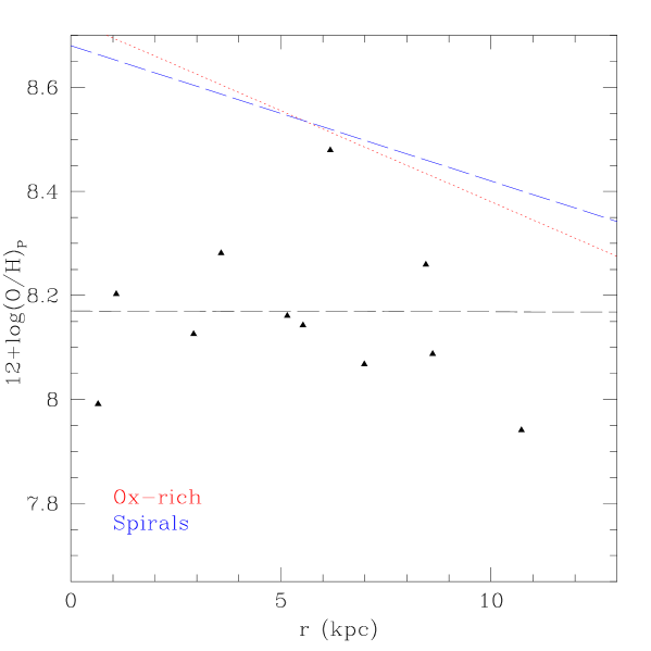
Figure 6: Oxygen abundance derived with empirical methods proposed by Pilyugin (2001) versus radius. The values in Tab. 4 were binned each 5 arcseconds. The superimposed lines are the linear best fit derived by Pilyugin et al. (2006); the red line represents the best fit to the abundance of oxygen-rich spirals, while the blue line is those related to ordinary spirals. The black line is the best fits obtained for NGC4650A.

where $P=R_{3}/R_{23}$. It can be used for oxygen abundance determination in moderately high-metallicity HII regions with undetectable or weak temperature-sensitive line ratios (Pilyugin, 2001).
We used also the ”P-method” to derive the oxygen abundance in the polar disk of NGC4650A: the values of $12+log(O/H)_{P}$ at each distance from the galaxy center are listed in Tab. 4, and shown in Fig. 5 and Fig. 6. The average value of the oxygen abundance is $12+log(O/H)_{P}=8.2\pm 0.2$, which is consistent with the values derived by using the Sulphur abundance parameter (Eq. 1).

The metallicities corresponding to each value of oxygen abundances given before have been estimated. We adopted $12+log(O/H)_{\odot}=8.83=A_{\odot}$ and $Z_{\odot}=0.02$ (Asplund et al., 2004). Given that $Z_{NGC4650A}\approx KZ_{\odot}$ and $K=10^{[A_{NGC4650A}-A_{\odot}]}$, we obtain a metallicity for the HII regions of the polar disk in NGC4650A $Z\simeq 0.004$ which correspond to $Z\simeq(0.2\pm 0.002)Z_{\odot}$.

3.2 Direct oxygen abundance measurements

The electron temperature is the fundamental parameter to directly derive the chemical abundances in the star-forming regions of galaxies. In a temperature-sensitive ion, with a well separated triplet of fine-structure terms, electron temperature and electron density ($N_{e}$), can be measured from the relative strengths of lines coming from excited levels at different energies above the ground state (see Osterbrock 1989; Allen 1984). As explained in detail below, the oxygen abundances are function of both the emission line fluxes and electron temperatures: this relation is the basis of the commonly known as direct method or $T_{e}$ method.
Usually, it happens that not all these lines can be observed in the spectra, or they are affected by large errors. Thus, some assumption were proposed for the temperature structure through the star-forming region: for HII galaxies it is assumed a two-zone model with a low ionization zone, where the OII, NII, NeII and SII lines are formed, and a high ionization zone where the OIII, NIII, NeIII and SIII lines are formed (see, e.g. Campbell et al. 1986; Garnett 1992). Photoionization models are then used to relate the temperature of the low ionization zone $t_{2}$ to $t_{3}$, the temperature of the high ionization zone (Pagel et al. 1992; Pérez-Montero & Díaz 2003; Pilyugin et al. 2006; Pilyugin 2007; Pilyugin et al. 2009).

For NGC4650A, we aim to derive the oxygen abundance of the polar disk directly by the estimate of the $O^{++}$ and $O^{+}$ ions electron temperatures. According to Izotov et al. (2005) and Pilyugin et al. (2006), we have adopted the following equations for the determination of the oxygen abundances, which are based on a five-level atom approximation:

$$12+log(OIII/H)=log([4959+5007]/H_{\beta})+6.2+1.251/t_{3}-0.55logt_{3}-0.014t_{3}$$ (3)

$$12+log(OII/H)=log([3727]/H_{\beta})+5.961+1.676/t_{2}-0.40logt_{2}-0.034t_{2}+log(1+1.35x_{2})$$ (4)

where $t_{3}$ and $t_{2}$ are the electron temperatures within the [OIII] and [OII] zones respectively, in units of $10^{4}$ K; $x_{2}=10^{-4}N_{e}t_{2}^{-0.5}$, where $N_{e}$ is the electron density. The total oxygen abundance is $O/H=OIII/H+OII/H$.

The electron temperatures and the electron density, needed to solve the above relations, have been derived using the task TENDEM of the STSDAS package in IRAF, which solves the equations of the statistical equilibrium within the five-level atom approximation (De Robertis et al. 1987; Shaw & Dufour 1995). According to this model, both $t_{3}$ and $t_{2}$ are function of the electron density $N_{e}$ and of the line ratios $R_{OIII}=[OIII]\lambda(4959+5007)/[OIII]\lambda 4363$ and $R_{OII}=[OII]\lambda 3727/[OII]\lambda 7325$, respectively. For NGC4650A, $N_{e}$ has been derived from the line ratio $[SII]\lambda 6717/[SII]\lambda 6731$, which has the average value of $0.83\pm 0.06$, through the whole disk extension, for a default temperature of $10^{4}$ K. This let to $N_{e}\sim 1217$ $cm^{-3}$. Even though the auroral line $[OIII]\lambda 4363$ is usually very weak, even in the metal-poor environments, the large collecting area of the 8m telescope and the high signal-to-noise spectra, let us to measure such emission line along the whole extension of the polar disk (see Tab. 2), which let us to estimate $R_{OIII}$.
The electron temperature $t_{3}=f(R_{OIII},N_{e})$ has been calculated by putting $N_{e}$ and $R_{OIII}$ as inputs in the TENDEM task: given the large spread of $R_{OIII}$, we adopted the average value in the following three bins, $0\leq R\leq 20$ arcsec, $20<R\leq 40$ arcsec, $40<R\leq 60$ arcsec. The distribution of $t_{3}$ in each bin is shown in Fig. 7: the electron temperature is almost constant till about 40 arcsec and tends to increase at larger distances. In the same figure there are also plotted the values of $t_{2}$ (at the same distances) obtained by adopting the following empirical $t_{2}-t_{3}$ relation, derived by Pilyugin et al. (2009): $t_{2}=0.264+0.835t_{3}$. The empirical $t_{2}-t_{3}$ relation has been investigated and debated for a long time and several forms are given in the literature; that by Pilyugin et al. (2009) is the most recent work on this subject, where they derived the $t_{2}-t_{3}$ relation in terms of the nebular $R_{3}=[OIII]\lambda(4959+5007)/H_{\beta}$ and $R_{2}=[OII]\lambda 3727/H_{\beta}$ line fluxes. They found that such relation is valid for HII regions with a weak nebular $R_{3}$ lines ($logR_{3}\geq 0.5$) and it turns to be consistent with those commonly used (see Fig. 14 in Pilyugin et al. (2009) paper and reference therein). The polar disk of NGC4650A, since $logR_{3}=0.5\pm 0.2$ (this is the average value on the whole disk extension), is located in the upper validity limit of the $t_{2}-t_{3}$ relation.
This is what is usually done since the auroral line $[OII]\lambda 7325$ is too weak to obtain a good enough estimate of the electron temperature $t_{2}$. For the polar disk of NGC4650A, the line fluxes of $[OII]\lambda(7320+7330)$ are strong enough to be measured at about 30 arcsec and the average value of $[OII]\lambda(7320+7330)/H_{\beta}=0.04\pm 0.01$. The average value of the ratio $R_{OII}=[OII]\lambda 3727/[OII]\lambda 7325$ is given as input in the TENDEM task, and we obtain $t_{2}=(1.092\pm 0.20)\times 10^{4}$ K, which is added to Fig. 7. This value is lower than that derived by using photoionization models, even if the observed and theoretical values of $t_{2}$ are consistent within errors: such difference could be due both to the uncertainties in the line fluxes measurements, made on so few and weak lines, and to the validity limit of the $t_{2}-t_{3}$ relation.
To obtain the oxygen abundance for the polar disk, we decided to adopt both estimates for $t_{2}$, by using the average value inside 40 arcsec for that derived by photoionization models, which is $t_{2}^{mod}=(1.7\pm 0.2)\times 10{{}^{4}}$ K, and, consistently, an average value for $t_{3}=(2.0\pm 0.2)\times 10{{}^{4}}$ K at the same distances. By adopting the Eq. 3 and Eq. 4, the oxygen abundance $12+log(O/H)_{T}$ for the polar disk is shown in Fig. 8 and listed in Tab. 5. By using the value of $t_{2}$ derived by direct measurements of OII line fluxes, the metallicity is higher with respect to that derived by using the value of $t_{2}$ from photoionization models: the average value is $12+log(O/H)_{T_{obs}}=8.4\pm 0.1$ and $12+log(O/H)_{T_{mod}}=7.6\pm 0.5$ for the two cases respectively. The large error, that are derived by propagating the emission line intensity errors listed in Tab. 2 and Tab. 3, which is about 0.5, let both estimates consistent.
It is important to point out that the oxygen abundance derived by direct measurements of OII line fluxes for $t_{2}$ is much more similar to the value derived by empirical methods, which is $12+log(O/H)=8.3$, than the value derived by using photoionization models for $t_{2}$: this may suggest that NGC4650A could be out of the range of validity of these models.

4 Discussion: use of the chemical analysis to constrain the galaxy formation

As discussed above, we derive the oxygen abundance, $12+log(O/H)$ to be $8.2\pm 0.1$, by using both the empirical and direct methods. In the following sections we will discuss the results obtained by the present work, how they could reconcile with the predictions by theoretical models and, finally, we address the main conclusions of this study.

4.1 Results

Here we discuss how the average value of metallicity and its distribution along the polar disk compares with those typical for other late-type disk galaxies and PRGs.

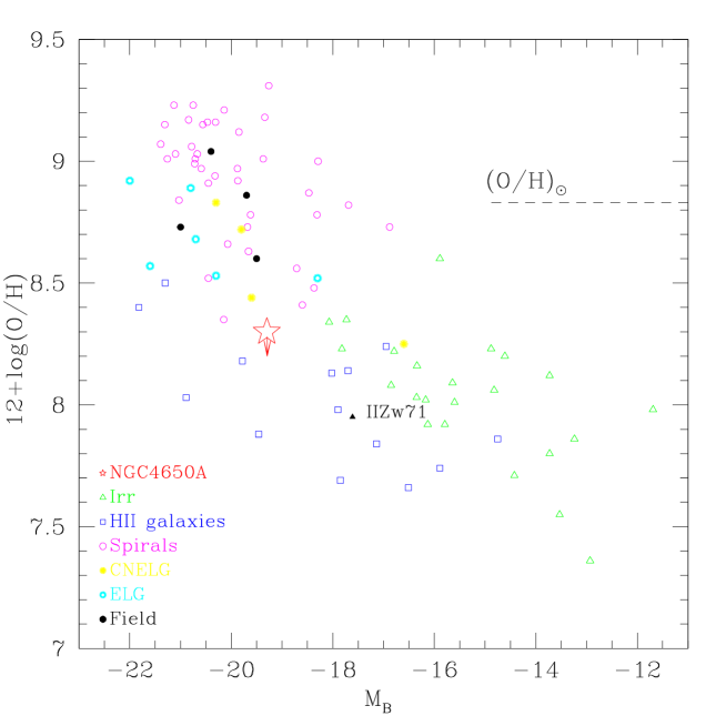
Figure 9: Oxygen abundance vs absolute blue magnitude for CNELGs (yellow filled circles), ELGs (cyan open circles), four field galaxies with emission lines (filled black circles), nearby dwarf irregulars (open triangles), local spiral galaxies (open circles), local HII galaxies (open squares), NGC4650A (star) and the polar disk galaxy IIZw71 (Perez-Montero et al., 2009). The dashed line indicates the solar oxygen abundance. The arrow indicates the shift of the value of the oxygen abundance if we use the direct methods to evaluate it. The total B-band magnitude for NGC4650A ($M_{B}=-19.3$) has been evaluated by using the same value of $H_{0}$ used by Kobulnicky & Zaritsky (1999) in order to compare NGC4650A with galaxies in their sample

- Metallicity-Luminosity relation
The mean values for the oxygen abundance along the polar disk, derived by the empirical (see Sec. 3.1) and direct methods (see Sec. 3.2), are compared with those for a sample of late-type disk galaxies by Kobulnicky & Zaritsky (1999), as function of the total luminosity (see Fig. 9). For all galaxies of the sample, and in particular for spiral galaxies, the total luminosity is that of the whole system, i.e. bulge plus disk, therefore also for NGC4650A we have accounted for the total luminosity of the galaxy ($M_{B}=-19.3$, evaluated by using the same value of $H_{0}$ used by Kobulnicky & Zaritsky (1999) in order to compare NGC4650A with galaxies in their sample), to which contributes both the central spheroid and the polar disk. We found that NGC4650A is located inside the spread of the data-points and contrary to its high luminosity it has metallicity lower than spiral galaxy disks of the same total luminosity. If we take into account the total luminosity of the polar disk alone ($M_{B}=-17$), NGC4650A falls in the region where HII and irregular galaxies are also found, characterized by lower luminosity and metallicities with respect to the spiral galaxies.
For what concerns the chemical abundances in PRGs, only few measurements are available in the literature. By using the direct method, very recently Perez-Montero et al. (2009) have derived the chemical abundances of IIZw71, a blue compact dwarf galaxy also catalogued as a probable polar ring: consistently with its low luminosity, the metallicity of the brightest knots in the ring is lower with respect to that of NGC4650A. Through a similar study, Brosch et al. (2009) have derived the chemical abundances for the apparent ring galaxy SDSS J075234.33+292049.8, which has a more similar morphology to that observed in NGC4650A: the average value for the oxygen abundance along the polar structure is $12+logO/H=8.49\pm 0.08$. As pointed out by authors, taking into account the ring brightness, such value is somewhat lower than that expected by the metallicity-luminosity relation. A spectroscopic study of the peculiar galaxy UGC5600, classified as probable PRG (Whitmore et al., 1990), by Shalyapina et al. (2002) reports a quasi-solar metallicity for such object, $12+log(O/H)\sim 8.8=0.9Z_{\odot}$, which is consistent with its high luminosity ($M_{B}=-19.4$), but it is larger with respect to the values of other PRGs given before.

- Metallicity gradient along the polar disk
The oxygen abundance in the polar disk of NGC4650A as a function of the radius derived by empirical and direct methods are shown in Fig. 6 and Fig. 8 respectively: both of them show that metallicity remains constant along the polar disk. This suggests that the star formation and metal enrichment in the polar structure of NGC4650A is not influenced by the stellar evolution of the older central spheroid, where the last burst of star formation occurred between 3 to 5 Gyrs ago (Iodice et al., 2002): this turns also to be consistent with a later formation of the polar disk. The absence of any metallicity gradient is a typical behavior found in LSB galaxies (de Blok & van der Hulst, 1998), and also in the polar disk galaxy studied by Brosch et al. (2009), which has a very similar structure to NGC4650A. On the contrary, ordinary and oxygen-rich spiral galaxies show a decreasing abundance with increasing radii (see Fig. 6 and Pilyugin et al. 2006). These observed features in spiral disks are well explained by the infall models of galaxy formation which predict that they build up via accretion by growing inside-out (Matteucci & Francois 1989; Boissier & Prantzos 1999) and such process generates the observed gradients.

- Star Formation Rate (SFR)
We have derived the SFR for the polar disk, from the $H_{\alpha}$ luminosity using the expression given by Kennicutt (1998) $SFR(M_{\odot}/yr)=7.9\times 10^{-42}\times L(H_{\alpha})(erg/s)$. We found that it is almost constant along the disk, within a large scatter of the datapoint. Therefore, given the average value of $L(H_{\alpha})\simeq 3.8\times 10^{39}$ erg/s we have obtained an average $SFR\sim 0.04M_{\odot}/yr$ and $SFR\sim 0.02M_{\odot}/yr$ for the North and South arms respectively. These values are quite similar to the total SFR derived for the HII regions of PRG IIZw71 (Perez-Montero et al. 2009), which is $SFR\sim 0.035M_{\odot}/yr$. In order to make a comparison with SFR estimates for a sample of PRGs studied by Reshetnikov & Combes (1994), we have derived a mean value of the $H_{\alpha}$ flux by integrating within a rectangular aperture of $2.5^{\prime\prime}\times 4.6^{\prime\prime}$ along each arm of the polar disk and we have obtained an average value of $SFR\sim 0.006M_{\odot}/yr/pc^{2}$. This value is consistent with the SFR of the HII regions in the PRGs studied by Reshetnikov & Combes (1994), where $0.001\leq SFR\leq 0.31$. In particular, two PRGs of this sample, UGC7576 and UGC9796, where the polar structure is very similar to that of NGC4650A (i.e. exponential surface brightness profile, very blue colors, knotty appearance, prominent HII regions and a large amount of HI gas, all associated to this component and distributed as a disk in differential rotation; see Reshetnikov & Combes 1994 and Cox et al. 2006), have $SFR\sim 0.005M_{\odot}/yr/pc^{2}$. As already stressed by Reshetnikov & Combes (1994), the HII regions of the PRGs, including also NGC4650A, have SFR similar to late-type spiral galaxies (Kennicutt et al., 1987). In particular, by comparing the $H_{\alpha}$ luminosity versus the total B magnitude, the polar disk galaxies, NGC4650A, UGC7576 and UGC9796, are located in the same area where Sc-Irr galaxies are also found.

Taking into account that the polar disk is very young, since the last burst of star formation occurred less than 1 Gyr ago (Iodice et al., 2002), we check if the present SFR of 0.06 $M_{\odot}/yr$, and even 2 and 3 times higher (i.e. $SFR=0.12M_{\odot}/yr$ and $SFR=0.18M_{\odot}/yr$), can give the estimated metallicity of $Z=0.2Z_{\odot}$ and how strongly could increase the metallicity with time. We used a linearly declining SFR (Bruzual & Charlot, 2003) $\psi(t)=2M_{\star}\tau^{-1}[1-(t/\tau)]$ (typically used for late-type galaxies), to estimate the expected stellar mass for the three different values of the SFR (0.06, 0.12 and 0.18 $M_{\odot}/yr$) and three epochs (0.8 Gyr, 1 Gyr and 2 Gyrs), obtaining stellar masses in the range $4\times 10^{9}M_{\odot}\leq M_{\star}\leq 1\times 10^{10}M_{\odot}$. The stellar mass ($M_{\star}\sim 4\times 10^{9}M_{\odot}$) in the disk from NIR observations (Iodice et al., 2002) falls within this range. Than, by using the mass-metallicity relation derived by Tremonti et al. (2004), where $12+log(O/H)=-1.492+1.847log(M_{\star})-0.08026(logM_{\star})^{2}$, we found that $1.02Z_{\odot}\leq Z\leq 1.4Z_{\odot}$. This shows that the present SFR for the polar disk ($SFR=0.06M_{\odot}yr^{-1}$) is able to increase the metallicity of about $0.2Z_{\odot}$ after 1Gyr. The derived values for Z are larger than $Z=(0.2\pm 0.002)Z_{\odot}$, found by using the element abundances (see Sec.3.1): this differences could be attributed to the accretion of metal-poor gas, as discussed in detail in the following sections.

4.2 Theoretical predictions

How galaxies acquire their gas is an open issue in the models of galaxy formation and recent theoretical works have argued that cold accretion plays a major role. This idea is supported by many numerical simulations suggesting that this could be an important mechanism in the galaxy formation (Katz & White 1993; Katz et al. 1994; Kereš et al. 2005; Dekel & Birnboim 2006; Dekel & Birnboim 2008; Bournaud & Elmegreen 2009). Kereš et al. (2005) studied in detail the physics of the cold mode of gas accretion and one feature they found is that it is generally directed along filaments, allowing galaxies to draw gas from large distances.
Recently Ocvirk et al. (2008), using cosmological simulations, studied the metal enrichment of the intergalactic medium as a key ingredient in determining the transition mass from cold to hot dominated accretion. Their measurements turn to be consistent with the analytical prediction of Dekel & Birnboim (2006) in the low metallicity regime for the cold streams. The efficiency of radiative cooling decreases towards low metallicity, and at $Z/Z_{\odot}=10^{-3}$ the cooling properties of the gas are those of a primordial mixture. Gas accretion is bimodal both in temperature and in metallicity: the cold accretion mode is associated with a combination of metal-poor filamentary accretion and dense metal-rich satellite galaxy disc surrounding, while the hot mode features has strong chemical heterogeneity and a radius-dependent metallicity.

More recent simulations of disk formation in a cosmological context performed by Agertz et al. (2009) revealed that the so called chain-galaxies and clump-clusters, found only at higher redshifts (Elmegreen et al., 2007), are a natural outcome of early epoch enhanced gas accretion from cold dense streams as well as tidally and ram-pressured stripped material from minor mergers and satellites. This freshly accreted cold gas settles into a large disk-like systems; simulations show that the interaction region between the new-formed disk and the cold streams can also result not aligned with the initial galactic disk: based on a very poor statistics, Agertz et al. (2009) suggest that this misalignment might not be typical, and it is due to a third cold stream that is perpendicular to the main filament. A more recent analysis by Dekel et al. (2009) shows that the accretion of gas along misaligned filaments with respect to the disk plane are more common and it leaves traces down to low redshift. An almost polar filament can result just as an extreme case of such process and, as suggested by Agertz et al. (2009), it could be responsible for the formation of polar disks.
This scenario not only reproduces the observed morphology and global rotation of disks, but also finds a realistic metallicity gradient and SFR of $20M_{\odot}/yr$. Agertz et al. (2009) found solar metallicity for the inner disk, while that in the clump forming region is only $\sim 1/10Z_{\odot}$ due to the accretion of pristine gas in the cold streams mixing with stripped satellite gas. Therefore, the studies cited above suggest that the chemical abundance is one of the key parameters that can be estimated in a galaxy disk and directly compared with the theoretical predictions. This is the main goal of the present work: we studied the chemical abundances in the polar disk of NGC4650A in order to check the cold accretion scenario for this object.

Hydrodynamical simulations performed by Macciò et al. (2006) and Brook et al. (2008) have shown that the formation of a polar disk galaxy can occur naturally in a hierarchical universe, where most low-mass galaxies are assembled through the accretion of cold gas infalling along a filamentary structures. According to Macciò et al. (2006), the polar disk forms from cold gas that flows along the extended $\sim 1Mpc$ filament into the virialized dark matter halo. The gas streams into the center of the halo on an orbit that is offset from radial infall. As it reaches the center, it impacts with gas in the halo of the host galaxy and with the warm gas flowing along the opposite filament. Only the gas accreted perpendicular to the major axis of the potential can survive for more than a few dynamical lifetimes.
Brook et al. (2008) argued that polar disk galaxies are extreme examples of the misalignment of angular momentum that occurs during the hierarchical structure formation: an inner disk starts forming shortly after the last major merger at $z\sim 2$. Due to its gas rich nature, the galaxy rapidly forms a new disk whose angular momentum is determined by the merger orbital parameters. Later, gas continues to be accreted but in a plane that is almost perpendicular to the inner disk. At $z\sim 0.8$ the central galaxy is still forming stars in a disk, while the bulk of new star formation is in the highly inclined polar disk. By $z\sim 0.5$ the inner disk has exhausted its gas, while gas continues to fall onto the polar disk. From this point, star formation occurs exclusively in the polar disk, that remains stable for at least 3 Gyrs.
The formation mechanisms described above can self-consistently explain both morphology and kinematics of a polar disk galaxy and, in particular, all the observed features (like colors and color gradients, longevity, spiral arms, HI content and distribution) of the polar structure.

5 Summary and conclusions

The present study could be considered a step forward both to trace the formation history of NGC4650A and to give hints on the mechanisms at work during the building of a disk by cold accretion process.

As mentioned in the Sec.1, the new kinematic data obtained for the central spheroid (Iodice et al., 2006), together with the previous studies, set important constraints on the possible formation mechanisms for NGC4650A. In particular, the merging scenario is ruled out because, according to simulations (e.g. Bournaud et al. 2005), a high mass ratio of the two merging galaxies is required to form a massive and extended polar disk as observed in NGC 4650A: this would convert the intruder into an elliptical-like, not rotationally supported, stellar system. This is in contrast with the high maximum rotation velocity ($\sim 80\div 100$ km/s) observed in the outer regions of the central spheroid (Iodice et al., 2006).

Both the high baryonic mass (star plus gas) in the polar structure and its large extension cannot reconcile with a polar ring formed via the gradual disruption of a dwarf satellite galaxy (as explained by Iodice et al. 2002). Differently, a wide polar ring and/or disk (as observed in NGC4650A) may form both around a disk or an elliptical galaxy through the tidal accretion of gas stripped from a gas-rich donor, in the case of large relative velocity and large impact parameter and for a particular orbital configuration (e.g. Bournaud & Combes 2003). Therefore, the two formation scenarios which can be really envisioned in the specific case of NGC4650A are the tidal accretion and the accretion of external primordial cold gas from cosmic web filaments (Macciò et al. 2006; Brook et al. 2008). To this aim we have derived the metallicity and SFR for the polar disk in NGC4650A in order to compare them with those predicted by different formation scenarios.

The main results of the present work are (see also Sec. 4.1): i) the low value of the metallicity derived for the polar disk $Z=0.2Z_{\odot}$, in spite of its high luminosity, $M_{B}=-19.3$ (see Fig. 9), ii) the lack of any metallicity gradient along the polar disk, which suggests that the metal enrichment is not influenced by the stellar evolution of the older central spheroid, iii) the metallicities expected for the present SFR at three different epochs, $1.02Z_{\odot}\leq Z\leq 1.4Z_{\odot}$, are higher than those measured from the element abundances and this is consistent with a later infall of metal-poor gas.

In the following we will address how these results reconcile with the predictions by theoretical models (see Sec. 4.2) and may discriminate between the two formation mechanisms.

If the polar ring/disk formed by the mass transfer from a gas-rich donor galaxy, the accreted material comes only from the outer and more metal-poor regions of the donor: is the observed metallicity for the polar component in NGC4650A consistent with the typical values for the outer disk of a bright spiral galaxy? According to Bresolin et al. (2009), the metallicity of very outer regions of a bright spiral is $0.2Z_{\odot}\leq Z\leq 1.1Z_{\odot}$: the observed value for NGC4650A, $Z=0.2Z_{\odot}$, is close to the lower limit.
The cold accretion mechanism for disk formation predicts quite low metallicity ($Z=0.1Z_{\odot}$) (Dekel & Birnboim 2006, Ocvirk et al. 2008, Agertz et al. 2009): such value refers to the time just after the accretion of a misaligned material, so it can be considered as initial value for Z before the subsequent enrichment. How this may reconcile with the observed metallicity for NGC4650A? We estimated that the present SFR for the polar disk ($SFR=0.06M_{\odot}yr^{-1}$) is able to increase the metallicity of about 0.2 after 1Gyr (see Sec.4.1): taking into account that the polar structure is very young, less than 1Gyr (Iodice et al., 2002), an initial value of $Z=0.1Z_{\odot}$, at the time of polar disk formation, could be consistent with the today’s observed metallicity.
This evidence may put some constraints also on the time-scales of the accretion process. The issue that need to be addressed is: how could a cosmic flow form a ring/disk only in the last Gyr, without forming it before? Given that the average age of 0.8 Gyr refers to the last burst of star formation, reasonably the gas accretion along the polar direction could have started much earlier and stars formed only recently, once enough gas mass has been accumulated in the polar disk. Earlier-on, two possible mechanisms may be proposed. One process that may happen is something similar to that suggested by Martig et al. (2009) for the quenching of star formation in early-type galaxies: given that star formation takes place in gravitationally unstable gas disks, the polar structure could have been stable for a while and this could have quenched its star formation activity, until the accumulated mass gas exceeds a stability threshold and star formation resumes. Alternatively, according to the simulations by Brook et al. (2008), the filament could have been there for several Gyrs with a relative low inclination, providing gas fuel to the star formation in the host galaxy first, about 3 Gyrs ago. Then large-scale tidal fields can let the disk/filament misalignment increase over the time till 80-90 degrees and start forming the polar structure during the last 1-2 Gyrs. This picture might be consistent not only with the relative young age of the polar disk, but also with the estimate of the last burst of star formation in the central spheroid (Iodice et al., 2002).

One more hint for the cold accretion scenario comes from the fact that the metallicity expected by the present SFR turns to be higher than those directly measured by the chemical abundances. As suggested by Dalcanton (2007), both infall and outflow of gas can change a galaxy’s metallicity: in the case of NGC4650A a possible explanations for this difference could be the infall of pristine gas, as suggested by (Finlator et al. 2007; Ellison et al. 2008).

The lack of abundance gradient in the polar disk, as typically observed also in LSB galaxies, suggests that the picture of a chemical evolution from inside-out, that well reproduce the observed features in spiral disks (Matteucci & Francois 1989, Boissier & Prantzos 1999), cannot be applied to these systems. In particular, observations for LSB galaxies are consistent with a quiescent and sporadic chemical evolution, but several explanation exist that supports such evidence (de Blok & van der Hulst, 1998). Among them, one suggestion is that the disk is still settling in its final configuration and the star formation is triggered by external infall of gas from larger radii: during this process, gas is slowly diffusing inward, causing star formation where conditions are favorable. As a consequence, the star formation is not self-propagating and the building-up of the disk would not give rise to an abundance gradient. The similarities between LSB galaxies and the polar disk in NGC4650A, including colors (Iodice et al., 2002) and chemical abundances (this work), together with the very young age of the polar disk, the presence of star forming regions towards larger radii, the warping structure of outer arms (Gallagher et al. 2002, Iodice et al. 2002), and the constant SFR along the disk (this work), suggest that the infall of metal-poor gas, through a similar process described above, may reasonably fit all these observational evidences.

Given that, are there any other observational aspects that can help to disentangle in a non ambiguous way the two scenarios?

One important feature which characterize NGC4650A is the high baryonic (gas plus stars) mass in the polar structure: it is about $12\times 10^{9}M_{\odot}$, which is comparable with or even higher than the total luminous mass in the central spheroid (of about $5\times 10^{9}M_{\odot}$). In the accretion scenario, the total amount of accreted gas by the early-type object is about $10\%$ of the gas in the disk donor galaxy, i.e. up to $10^{9}$ $M_{\odot}$, so one would expect the accreted baryonic mass (stellar + gas) to be a fraction of that in the pre-existing galaxy, and not viceversa, as it is observed for NGC4650A. Furthermore, looking at the field around NGC4650A, the close luminous spiral NGC4650 may be considered as possible donor galaxy (Bournaud & Combes, 2003), however the available observations on the HI content for this object show that NGC4650 is expected to be gas-poor (Arnaboldi et al. 1997; van Driel et al. 2002). So, where the high quantity of HI gas in NGC4650A may come from? If the polar disk forms by the cold accretion of gas from filaments there is no limit to the accreted mass.

Given all the evidences shown above, we can infer that the cold accretion of gas by cosmic web filaments could well account for both the low metallicity, the lack of gradient and the high HI content in NGC4650A. An independent evidence which seems to support such scenario for the formation of polar disks comes from the discovery and study of an isolated polar disk galaxy, located in a wall between two voids (Stanonik et al., 2009): the large HI mass (at least comparable to the stellar mass of the central galaxy) and the general underdensity of the environment can be consistent with the cold flow accretion of gas as possible formation mechanism for this object.

The present work remarks how the use of the chemical analysis can give strong constraints on the galaxy formation, in particular, it has revealed an independent check of the cold accretion scenario for the formation of polar disk galaxies. This study also confirmed that this class of object needs to be treated differently from the polar ring galaxies, where the polar structure is more metal rich (like UGC5600, see Sec. 4.1) and a tidal accretion or a major merging process can reliable explain the observed properties (Bournaud & Combes, 2003). Finally, given the similarities between polar disks and late-type disk galaxies, except for the different plane with respect to the central spheroid, the two classes of systems could share similar formation processes. Therefore, the study of polar disk galaxies assumes an important role in the wide framework of disk formation and evolution, in particular, for what concern the “rebuilding” of disks through accretion of gas from cosmic filaments, as predicted by hierarchical models of galaxy formation (Steinmetz & Navarro, 2002).

Table 1: General properties of NGC4650A

Parameter	Value	Ref.
Morphological type	PRG	NED
R.A. (J2000)	12h44m49.0s	NED
Dec. (J2000)	-40d42m52s	NED
Helio. Radial Velocity	2880 km/s	NED
Redshift	0.009607	NED
Distance	38 Mpc
Total mB (mag)	14.09 $\pm$ 0.21	NED
$M(HI)(M_{\bigodot})$	$8\times\ 10^{9}$	Arnaboldi et al. (1997)
$L_{B}(L_{\bigodot})$	$3\times\ 10^{9}$

Table 2: Observed and de-reddened emission lines fluxes relative to $H_{\beta}$ in the $3300-6210$ Å wavelength range.

r (arcsec)	OII[3727]/$H_{\beta}$		$H_{\gamma}$[4340]/$H_{\beta}$		OIII[4363]/$H_{\beta}$		OIII[4959]/$H_{\beta}$		OIII[5007]/$H_{\beta}$
slit1	$F_{obs}$	$F_{int}$	$F_{obs}$	$F_{int}$	$F_{obs}$	$F_{int}$	$F_{obs}$	$F_{int}$	$F_{obs}$	$F_{int}$
	$\pm 0.05$	$\pm 0.06$	$\pm 0.013$	$\pm 0.015$	$\pm 0.004$	$\pm 0.005$	$\pm 0.02$	$\pm 0.02$	$\pm 0.03$	$\pm 0.03$
-44.1	5.95	7.76	$\cdots$	$\cdots$	0.058	0.066	0.52	0.51	1.83	1.77
-42.34	4.32	5.64	$\cdots$	$\cdots$	0.201	0.227	0.52	0.51	1.83	1.77
-40.57	4.01	5.22	0.392	0.445	0.182	0.205	0.58	0.57	1.97	1.91
-38.81	3.69	4.81	$\cdots$	$\cdots$	0.094	0.107	0.57	0.56	1.67	1.61
-37.04	3.61	4.71	0.438	0.497	0.096	0.109	0.80	0.78	1.91	1.85
-35.28	3.39	4.42	0.398	0.451	0.095	0.108	0.80	0.78	1.82	1.76
-33.52	3.42	4.45	0.329	0.373	0.064	0.073	0.79	0.78	1.87	1.81
-31.75	3.38	4.41	0.377	0.428	0.043	0.048	0.51	0.50	1.60	1.55
-29.99	3.47	4.52	0.423	0.480	0.038	0.043	0.54	0.52	1.58	1.53
-28.22	3.99	5.21	0.464	0.526	0.188	0.212	0.60	0.59	1.76	1.71
-17.64	4.06	5.29	0.400	0.454	0.105	0.119	1.05	1.03	3.11	3.01
-14.11	3.12	4.06	0.376	0.427	$\cdots$	$\cdots$	0.50	0.50	1.36	1.31
-3.528	4.35	5.67	$\cdots$	$\cdots$	$\cdots$	$\cdots$	0.81	0.80	2.51	2.43
26.46	$\cdots$	$\cdots$	0.348	0.395	$\cdots$	$\cdots$	$\cdots$	$\cdots$	$\cdots$	$\cdots$
28.22	$\cdots$	$\cdots$	0.540	0.613	$\cdots$	$\cdots$	$\cdots$	$\cdots$	$\cdots$	$\cdots$
37.04	3.39	4.42	$\cdots$	$\cdots$	$\cdots$	$\cdots$	1.79	1.75	5.33	5.16
38.81	3.94	5.13	$\cdots$	$\cdots$	$\cdots$	$\cdots$	1.92	1.88	6.85	6.63
45.86	2.41	3.14	$\cdots$	$\cdots$	$\cdots$	$\cdots$	0.24	0.24	0.51	0.49
47.63	4.33	5.64	$\cdots$	$\cdots$	0.030	0.034	0.21	0.20	0.37	0.36
49.39	3.70	4.82	$\cdots$	$\cdots$	$\cdots$	$\cdots$	0.20	0.20	0.33	0.32
slit 2
-49.49	$\cdots$	$\cdots$	0.598	0.678	$\cdots$	$\cdots$	$\cdots$	$\cdots$	$\cdots$	$\cdots$
-33.52	1.97	2.57	0.555	0.630	$\cdots$	$\cdots$	0.19	0.19	0.43	0.42
-31.75	2.24	2.91	$\cdots$	$\cdots$	$\cdots$	$\cdots$	0.17	0.17	0.54	0.53
-3.528	2.54	3.31	$\cdots$	$\cdots$	$\cdots$	$\cdots$	0.88	0.86	2.89	2.80
5.292	3.59	4.69	0.233	0.264	$\cdots$	$\cdots$	0.80	0.78	2.69	2.60
8.82	3.28	4.28	$\cdots$	$\cdots$	$\cdots$	$\cdots$	0.43	0.42	1.27	1.23
17.64	3.15	4.11	0.594	0.674	$\cdots$	$\cdots$	0.92	0.90	2.15	2.08
21.17	2.22	2.90	$\cdots$	$\cdots$	$\cdots$	$\cdots$	0.88	0.86	2.56	2.48
22.93	3.27	4.26	0.386	0.438	$\cdots$	$\cdots$	0.51	0.50	1.58	1.53
24.7	2.44	3.19	0.387	0.439	$\cdots$	$\cdots$	0.93	0.91	2.71	2.62
26.46	3.08	4.01	0.442	0.501	$\cdots$	$\cdots$	0.83	0.82	2.51	2.43
28.22	4.13	5.38	0.444	0.504	$\cdots$	$\cdots$	0.75	0.73	2.27	2.19
29.99	3.32	4.33	0.472	0.535	$\cdots$	$\cdots$	0.64	0.62	1.91	1.85
31.75	5.96	7.77	0.423	0.480	$\cdots$	$\cdots$	0.83	0.81	2.22	2.15
33.51	$\cdots$	$\cdots$	0.540	0.613	$\cdots$	$\cdots$	$\cdots$	$\cdots$	$\cdots$	$\cdots$
44.1	2.57	3.35	$\cdots$	$\cdots$	$\cdots$	$\cdots$	0.88	0.86	2.84	2.75
45.86	4.14	5.40	0.427	0.484	0.129	0.146	0.09	0.09	0.43	0.42
47.63	2.02	2.64	$\cdots$	$\cdots$	0.537	0.606	0.73	0.71	2.27	2.19
49.39	$\cdots$	$\cdots$	0.384	0.436	$\cdots$	$\cdots$	$\cdots$	$\cdots$	$\cdots$	$\cdots$
56.45	3.46	4.51	$\cdots$	$\cdots$	$\cdots$	$\cdots$	1.04	1.02	3.72	3.60
58.21	3.93	5.13	$\cdots$	$\cdots$	0.162	0.183	1.15	1.13	4.18	4.05
59.98	4.92	6.41	$\cdots$	$\cdots$	$\cdots$	$\cdots$	1.68	1.65	6.63	6.42

Table 3: Observed and de-reddened emission lines fluxes relative to $H_{\beta}$ in the $5600-11000$Å wavelength range.

r (arcsec)	$H_{\alpha}[6563]/H_{\beta}$		SII[6717]/$H_{\beta}$		SII[6731]/$H_{\beta}$		SIII[9069]/$H_{\beta}$		SIII[9532]/$H_{\beta}$
slit 1	$F_{obs}$	$F_{int}$	$F_{obs}$	$F_{int}$	$F_{obs}$	$F_{int}$	$F_{obs}$	$F_{int}$	$F_{obs}$	$F_{int}$
	$\pm 0.02$	$\pm 0.03$	$\pm 0.015$	$\pm 0.011$	$\pm 0.016$	$\pm 0.012$	$\pm 0.08$	$\pm 0.06$	$\pm 0.15$	$\pm 0.11$
-38.81	$\cdots$	$\cdots$	$\cdots$	$\cdots$	$\cdots$	$\cdots$	$\cdots$	$\cdots$	0.05	0.03
-37.04	5.46	4.25	$\cdots$	$\cdots$	$\cdots$	$\cdots$	$\cdots$	$\cdots$	$\cdots$	$\cdots$
-35.28	3.85	2.99	$\cdots$	$\cdots$	$\cdots$	$\cdots$	$\cdots$	$\cdots$	0.017	0.010
-33.52	2.44	1.896	$\cdots$	$\cdots$	$\cdots$	$\cdots$	$\cdots$	$\cdots$	0.04	0.03
-31.75	0.930	0.724	$\cdots$	$\cdots$	$\cdots$	$\cdots$	$\cdots$	$\cdots$	$\cdots$	$\cdots$
-29.99	0.412	0.321	$\cdots$	$\cdots$	$\cdots$	$\cdots$	$\cdots$	$\cdots$	$\cdots$	$\cdots$
-26.46	$\cdots$	$\cdots$	$\cdots$	$\cdots$	$\cdots$	$\cdots$	$\cdots$	$\cdots$	0.05	0.03
-17.64	$\cdots$	$\cdots$	$\cdots$	$\cdots$	$\cdots$	$\cdots$	$\cdots$	$\cdots$	0.03	0.019
-15.88	$\cdots$	$\cdots$	$\cdots$	$\cdots$	$\cdots$	$\cdots$	$\cdots$	$\cdots$	0.06	0.03
-10.58	$\cdots$	$\cdots$	0.199	0.153	0.632	0.483	$\cdots$	$\cdots$	$\cdots$	$\cdots$
-8.82	$\cdots$	$\cdots$	0.426	0.329	0.577	0.441	0.052	0.0320	$\cdots$	$\cdots$
-7.06	$\cdots$	$\cdots$	0.84	0.646	0.935	0.714	0.0293	0.0178	$\cdots$	$\cdots$
-5.29	$\cdots$	$\cdots$	$\cdots$	$\cdots$	$\cdots$	$\cdots$	0.041	0.0252	$\cdots$	$\cdots$
-3.53	$\cdots$	$\cdots$	$\cdots$	$\cdots$	$\cdots$	$\cdots$	0.68	0.41	$\cdots$	$\cdots$
-1.76	$\cdots$	$\cdots$	$\cdots$	$\cdots$	$\cdots$	$\cdots$	0.266	0.162	$\cdots$	$\cdots$
0.0	$\cdots$	$\cdots$	1.39	1.07	1.31	1.00	$\cdots$	$\cdots$	$\cdots$	$\cdots$
1.76	$\cdots$	$\cdots$	1.48	1.14	0.609	0.465	0.33	0.202	$\cdots$	$\cdots$
3.53	$\cdots$	$\cdots$	0.686	0.529	0.460	0.351	$\cdots$	$\cdots$	$\cdots$	$\cdots$
5.29	$\cdots$	$\cdots$	0.136	0.105	0.422	0.322	$\cdots$	$\cdots$	$\cdots$	$\cdots$
7.06	$\cdots$	$\cdots$	0.0142	0.0109	0.377	0.288	0.041	0.0249	0.023	0.014
29.99	$\cdots$	$\cdots$	$\cdots$	$\cdots$	$\cdots$	$\cdots$	$\cdots$	$\cdots$	0.014	0.008
31.75	$\cdots$	$\cdots$	$\cdots$	$\cdots$	$\cdots$	$\cdots$	$\cdots$	$\cdots$	0.022	0.013
40.57	$\cdots$	$\cdots$	0.0340	0.0262	0.174	0.133	$\cdots$	$\cdots$	$\cdots$	$\cdots$
51.16	$\cdots$	$\cdots$	0.465	0.358	0.280	0.214	0.33	0.202	1.0	0.6
slit 2
-45.86	$\cdots$	$\cdots$	$\cdots$	$\cdots$	$\cdots$	$\cdots$	$\cdots$	$\cdots$	0.11	0.06
-38.81	1.59	1.24	$\cdots$	$\cdots$	$\cdots$	$\cdots$	$\cdots$	$\cdots$	$\cdots$	$\cdots$
-37.04	5.48	4.26	$\cdots$	$\cdots$	$\cdots$	$\cdots$	$\cdots$	$\cdots$	$\cdots$	$\cdots$
-33.52	$\cdots$	$\cdots$	$\cdots$	$\cdots$	$\cdots$	$\cdots$	$\cdots$	$\cdots$	0.13	0.08
-22.93	0.874	0.680	$\cdots$	$\cdots$	$\cdots$	$\cdots$	$\cdots$	$\cdots$	$\cdots$	$\cdots$
-17.64	$\cdots$	$\cdots$	$\cdots$	$\cdots$	$\cdots$	$\cdots$	0.240	$\cdots$	$\cdots$
-5.29	$\cdots$	$\cdots$	0.0536	0.0413	0.271	0.207	$\cdots$	$\cdots$	0.22	0.1319
-3.53	$\cdots$	$\cdots$	0.090	0.070	0.0551	0.0421	$\cdots$	$\cdots$	$\cdots$	$\cdots$
-1.76	$\cdots$	$\cdots$	0.962	0.741	0.0023	0.00177	$\cdots$	$\cdots$	0.17	0.10
0.0	$\cdots$	$\cdots$	0.0691	0.0533	0.113	0.087	$\cdots$	$\cdots$	$\cdots$	$\cdots$
1.76	$\cdots$	$\cdots$	$\cdots$	$\cdots$	$\cdots$	$\cdots$	$\cdots$	$\cdots$	0.13	0.08
3.53	$\cdots$	$\cdots$	$\cdots$	$\cdots$	$\cdots$	$\cdots$	0.55	0.33	0.3	0.17
5.29	$\cdots$	$\cdots$	$\cdots$	$\cdots$	$\cdots$	$\cdots$	0.36	0.218	$\cdots$	$\cdots$
8.82	$\cdots$	$\cdots$	0.583	0.449	0.87	0.658	1.59	0.97	2	1.3
10.58	$\cdots$	$\cdots$	$\cdots$	$\cdots$	$\cdots$	$\cdots$	0.67	0.41	0.3	0.20
19.4	$\cdots$	$\cdots$	$\cdots$	$\cdots$	$\cdots$	$\cdots$	$\cdots$	$\cdots$	0.18	0.10
21.17	$\cdots$	$\cdots$	$\cdots$	$\cdots$	$\cdots$	$\cdots$	0.54	0.33	$\cdots$	$\cdots$
24.7	1.63	1.26	0.159	0.123	1.15	0.88	$\cdots$	$\cdots$	0.18	0.11
26.46	0.290	0.226	$\cdots$	$\cdots$	$\cdots$	$\cdots$	$\cdots$	$\cdots$	$\cdots$	$\cdots$
28.22	0.0620	0.0482	$\cdots$	$\cdots$	$\cdots$	$\cdots$	$\cdots$	$\cdots$	0.15	0.09
29.99	0.0938	0.0730	$\cdots$	$\cdots$	$\cdots$	$\cdots$	0.51	0.311	$\cdots$	$\cdots$
31.75	3.82	2.97	0.118	0.091	0.291	0.222	$\cdots$	$\cdots$	0.09	0.05
33.52	5.47	4.25	0.204	0.157	0.216	0.165	$\cdots$	$\cdots$	0.23	0.13
35.28	$\cdots$	$\cdots$	0.096	0.074	0.237	0.181	$\cdots$	$\cdots$	$\cdots$	$\cdots$
38.81	$\cdots$	$\cdots$	$\cdots$	$\cdots$	$\cdots$	$\cdots$	0.43	0.259	$\cdots$	$\cdots$
42.34	$\cdots$	$\cdots$	$\cdots$	$\cdots$	$\cdots$	$\cdots$	$\cdots$	$\cdots$	$\cdots$	$\cdots$
56.45	$\cdots$	$\cdots$	0.091	0.070	0.230	0.175	$\cdots$	$\cdots$	$\cdots$	$\cdots$
58.21	$\cdots$	$\cdots$	$\cdots$	$\cdots$	$\cdots$	$\cdots$	$\cdots$	$\cdots$	0.22	0.13
59.98	$\cdots$	$\cdots$	0.077	0.0587	0.134	0.102	0.37	0.226	$\cdots$	$\cdots$

Table 4: Oxygen and Sulphur abundance parameters and oxygen abundances for the polar disk in NGC4650A

r (arcsec)	$R_{23}$ ($\pm 0.05$)	$12+log(O/H)_{P}$ ($\pm 0.2$)
Slit 1
-44.1	10.05	7.8
-42.34	7.91	8.0
-40.57	7.70	8.1
-38.81	6.98	8.1
-37.04	7.35	8.1
-35.28	6.97	8.2
-33.52	7.04	8.2
-31.75	6.45	8.2
-29.99	6.57	8.2
-28.22	7.50	8.1
-17.64	9.33	8.0
-14.11	5.87	8.2
-3.528	8.90	8.0
37.04	11.33	8.0
38.81	13.64	7.8
45.86	3.86	8.4
47.63	6.20	8.0
49.39	5.34	8.1
Slit 2
-33.52	3.18	8.5
-31.75	3.61	8.4
-3.528	6.97	8.3
5.292	8.08	8.1
8.82	5.93	8.2
17.64	7.10	8.2
21.17	6.24	8.4
22.93	6.28	8.2
24.7	6.73	8.3
26.46	7.26	8.2
28.22	8.30	8.0
29.99	6.81	8.2
31.75	10.74	7.7
44.1	6.96	8.3
45.86	5.91	8.1
47.63	5.55	8.4
56.45	9.13	8.1
58.21	10.30	8.0
59.98	14.48	7.7

Table 5: Oxygen abundances for the polar disk in NGC4650A derived by the $T_{e}$ method

r (arcsec)	$12+log(O/H)_{T_{mod}}$	$12+log(O/H)_{T_{obs}}(\pm 0.1)$
Slit 1
-44.10	$7.83\pm 0.58$	8.6
-42.34	$7.71\pm 0.52$	8.5
-40.57	$7.69\pm 0.49$	8.5
-38.81	$7.65\pm 0.50$	8.4
-37.04	$7.67\pm 0.46$	8.4
-35.28	$7.64\pm 0.46$	8.4
-33.52	$7.65\pm 0.45$	8.4
-31.75	$7.62\pm 0.49$	8.4
-29.99	$7.63\pm 0.49$	8.4
-28.22	$7.69\pm 0.50$	8.5
-17.64	$7.76\pm 0.42$	8.5
-14.11	$7.58\pm 0.49$	8.4
-3.53	$7.75\pm 0.46$	8.5
37.04	$7.80\pm 0.33$	8.4
38.81	$7.88\pm 0.33$	8.5
45.86	$7.42\pm 0.58$	8.2
47.63	$7.64\pm 0.68$	8.5
49.39	$7.58\pm 0.67$	8.4
Slit 2
-33.52	$7.34\pm 0.57$	8.1
-31.75	$7.39\pm 0.57$	8.2
-3.53	$7.61\pm 0.36$	8.3
5.29	$7.70\pm 0.42$	8.4
8.82	$7.59\pm 0.52$	8.4
17.64	$7.64\pm 0.42$	8.4
21.17	$7.56\pm 0.35$	8.2
22.93	$7.61\pm 0.48$	8.4
24.70	$7.59\pm 0.36$	8.3
26.46	$7.64\pm 0.40$	8.4
28.22	$7.72\pm 0.47$	8.5
29.99	$7.63\pm 0.46$	8.4
31.75	$7.85\pm 0.54$	8.6
44.10	$7.61\pm 0.36$	8.3
45.86	$7.62\pm 0.68$	8.5
47.63	$7.51\pm 0.35$	8.2
56.45	$7.73\pm 0.37$	8.4
58.21	$7.78\pm 0.38$	8.5
59.98	$7.92\pm 0.36$	8.6

Figure 3: Top panel - Spectrum of NGC4650A in the blue wavelength range, corresponding to the region marked as A in the Fig. 1. Middle panel - Spectrum of the region B in the Fig. 1. Bottom panel - Spectrum of the region C in the Fig. 1, where are clearly visible the absorbing features of the line $H_{\gamma}$ and $H_{\beta}$.

Figure 4: Top panel - Spectra of NGC4650A in the red wavelength range, corresponding to the region marked as A in the Fig. 1. We divided the spectra in A1 and A2 in order to obtain a better visualization of the lines. Bottom panel - Spectrum of the region B (B1 and B2 as explained below) in the Fig. 1.

Figure 5: Oxygen abundance, obtained by using the empirical calibration introduced by Pilyugin (2001), versus oxygen abundance parameter $R_{23}$ (see Sec. 3.1).

Figure 7: Electron temperature along the polar disk of NGC4650A. The filled circles correspond to the observed T[OIII], the starred points correspond to the T[OII] estimated by the photoionization model (see Sec. 3.2 for details), the open square corresponds to the average value of T[OII] directly estimated by the ratio $R_{OII}=OII[3727]/[7325]$. In the bottom left side of the plot the mean error is shown.

Figure 8: Oxygen abundance derived with direct method. Squares are the values derived by using the observed $T[OII]$ estimates; stars are those derived by using the $T[OII]$ from photoionization models. See Sec. 3.2 for details. The errors on oxygen abundance is 0.5.

References

- Agertz et al. (2009) Agertz, O., Teyssier, R., & Moore, B. 2009, MNRAS, 397, L64
- Allen (1984) Allen, R. J. 1984, The Observatory, 104, 61
- Arnaboldi et al. (1997) Arnaboldi, M., Oosterloo, T., Combes, F., Freeman, K. C., & Koribalski, B. 1997, AJ, 113, 585
- Asplund et al. (2004) Asplund, M., Grevesse, N., Sauval, A. J., Allende Prieto, C., & Kiselman, D. 2004, A&A, 417, 751
- Bekki (1997) Bekki, K. 1997, ApJL, 490, L37
- Bekki (1998) Bekki, K. 1998, ApJ, 499, 635
- Bekki (1998) Bekki, K. 1998, ApJL, 502, L133
- Boissier & Prantzos (1999) Boissier, S., & Prantzos, N. 1999, MNRAS, 307, 857
- Bournaud & Combes (2003) Bournaud, F., & Combes, F. 2003, A&A, 401, 817
- Bournaud et al. (2007) Bournaud, F., Jog, C. J., & Combes, F. 2007, A&A, 476, 1179
- Bournaud et al. (2005) Bournaud, F., Jog, C. J., & Combes, F. 2005, A&A, 437, 69
- Bournaud & Elmegreen (2009) Bournaud, F., & Elmegreen, B. G. 2009, ApJL, 694, L158
- Bresolin et al. (2009) Bresolin, F., Ryan-Weber, E., Kennicutt, R. C., & Goddard, Q. 2009, ApJ, 695, 580
- Brook et al. (2008) Brook, C. B., Governato, F., Quinn, T., Wadsley, J., Brooks, A. M., Willman, B., Stilp, A., & Jonsson, P. 2008, ApJ, 689, 678
- Brosch et al. (2009) Brosch, N., Kniazev, A. Y., Moiseev, A., & Pustilnik, S. A. 2009, arXiv:0910.0589
- Bruzual & Charlot (2003) Bruzual, G., & Charlot, S. 2003, MNRAS, 344, 1000
- Buttiglione et al. (2006) Buttiglione, S., Arnaboldi, M., & Iodice, E. 2006, Memorie della Societa Astronomica Italiana Supplement, 9, 317
- Campbell et al. (1986) Campbell, A., Terlevich, R., & Melnick, J. 1986, MNRAS, 223, 811
- Cardelli et al. (1989) Cardelli, J. A., Clayton, G. C., & Mathis, J. S. 1989, ApJ, 345, 245
- Cole et al. (2000) Cole, S., Lacey, C. G., Baugh, C. M., & Frenk, C. S. 2000, MNRAS, 319, 168
- Conselice et al. (2003) Conselice, C. J., Bershady, M. A., Dickinson, M., & Papovich, C. 2003, AJ, 126, 1183
- Cox et al. (2006) Cox, A. L., Sparke, L. S., & van Moorsel, G. 2006, AJ, 131, 828
- Dalcanton (2007) Dalcanton, J. J. 2007, ApJ, 658, 941
- Davé et al. (2001) Davé, R., et al. 2001, ApJ, 552, 473
- de Blok & van der Hulst (1998) de Blok, W. J. G., & van der Hulst, J. M. 1998 A&A, 335, 421
- De Lucia et al. (2006) De Lucia, G., Springel, V., White, S. D. M., Croton, D., & Kauffmann, G. 2006, MNRAS, 366, 499
- De Robertis et al. (1987) De Robertis, M. M., Dufour, R. J., & Hunt, R. W. 1987, JRASC, 81, 195
- Dekel & Birnboim (2006) Dekel, A., & Birnboim, Y. 2006, MNRAS, 368, 2
- Dekel & Birnboim (2008) Dekel, A., & Birnboim, Y. 2008, MNRAS, 383, 119
- Dekel et al. (2009) Dekel, A., Sari, R., & Ceverino, D. 2009, ApJ, 703, 785
- Dekel et al. (2009) Dekel, A., et al. 2009, Nature, 457, 451
- Díaz & Pérez-Montero (2000) Díaz, A. I., & Pérez-Montero, E. 2000, MNRAS, 312, 130
- Ellison et al. (2008) Ellison, S. L., Patton, D. R., Simard, L., & McConnachie, A. W. 2008, ApJL, 672, L107
- Elmegreen et al. (2007) Elmegreen, D. M., Elmegreen, B. G., Ravindranath, S., & Coe, D. A. 2007, ApJ, 658, 763
- Finlator et al. (2007) Finlator, K., Davé, R., & Oppenheimer, B. D. 2007, MNRAS, 376, 1861
- Gallagher et al. (2002) Gallagher, J. S., Sparke, L. S., Matthews, L. D., Frattare, L. M., English, J., Kinney, A. L., Iodice, E., & Arnaboldi, M. 2002, ApJ, 568, 199
- Garnett (1992) Garnett, D. R. 1992, AJ, 103, 1330
- Genel et al. (2008) Genel, S., et al. 2008, ApJ, 688, 789
- Hägele et al. (2008) Hägele, G. F., Díaz, Á. I., Terlevich, E., Terlevich, R., Pérez-Montero, E., & Cardaci, M. V. 2008, MNRAS, 383, 209
- Hancock et al. (2009) Hancock, M., Smith, B. J., Struck, C., Giroux, M. L., & Hurlock, S. 2009, AJ, 137, 4643
- Hidalgo-Gámez & Ramírez-Fuentes (2009) Hidalgo-Gámez, A. M., & Ramírez-Fuentes, D. 2009, AJ, 137, 169
- Iodice et al. (2002) Iodice, E., Arnaboldi, M., De Lucia, G., Gallagher, J. S., III, Sparke, L. S., & Freeman, K. C. 2002, AJ, 123, 195
- Iodice et al. (2002) Iodice, E., Arnaboldi, M., Sparke, L. S., Gallagher, J. S., & Freeman, K. C. 2002, A&A, 391, 103
- Iodice et al. (2006) Iodice, E., et al. 2006, ApJ, 643, 200
- Izotov et al. (2005) Izotov, Y. I., Thuan, T. X., & Guseva, N. G. 2005, ApJ, 632, 210
- Katz & White (1993) Katz, N., & White, S. D. M. 1993, ApJ, 412, 455
- Katz et al. (1994) Katz, N., Quinn, T., Bertschinger, E., & Gelb, J. M. 1994, MNRAS, 270, L71
- Kennicutt et al. (1987) Kennicutt, R. C., Jr., Roettiger, K. A., Keel, W. C., van der Hulst, J. M., & Hummel, E. 1987, AJ, 93, 1011
- Kennicutt (1998) Kennicutt, R. C., Jr. 1998, ARA&A, 36, 189
- Kereš et al. (2005) Kereš, D., Katz, N., Weinberg, D. H., & Davé, R. 2005, MNRAS, 363, 2
- Keres (2008) Keres, D. 2008, 37th COSPAR Scientific Assembly, 37, 1496
- Kewley & Ellison (2008) Kewley, L. J., & Ellison, S. L. 2008, ApJ, 681, 1183
- Kobulnicky & Zaritsky (1999) Kobulnicky, H. A., & Zaritsky, D. 1999, ApJ, 511, 118
- Kobulnicky & Kewley (2004) Kobulnicky, H. A., & Kewley, L. J. 2004, ApJ, 617, 240
- Macciò et al. (2006) Macciò, A. V., Moore, B., & Stadel, J. 2006, ApJL, 636, L25
- Martig et al. (2009) Martig, M., Bournaud, F., Teyssier, R., & Dekel, A. 2009, ApJ, 707, 250
- Matteucci & Francois (1989) Matteucci, F., & Francois, P. 1989, MNRAS 239, 885
- Naab et al. (2007) Naab, T., Johansson, P. H., Ostriker, J. P., & Efstathiou, G. 2007, ApJ, 658, 710
- Ocvirk et al. (2008) Ocvirk, P., Pichon, C., & Teyssier, R. 2008, MNRAS, 390, 1326
- Osterbrock (1989) Osterbrock, D. E. 1989, Research supported by the University of California, John Simon Guggenheim Memorial Foundation, University of Minnesota, et al. Mill Valley, CA, University Science Books, 1989, 422 p.
- Pagel et al. (1979) Pagel, B. E. J., Edmunds, M. G., Blackwell, D. E., Chun, M. S., & Smith, G. 1979, MNRAS, 189, 95
- Pagel et al. (1992) Pagel, B. E. J., Simonson, E. A., Terlevich, R. J., & Edmunds, M. G. 1992, MNRAS, 255, 325
- Pérez-Montero & Díaz (2003) Pérez-Montero, E., & Díaz, A. I. 2003, MNRAS, 346, 105
- Pérez-Montero & Díaz (2005) Pérez-Montero, E., & Díaz, A. I. 2005, MNRAS, 361, 1063
- Perez-Montero et al. (2009) Perez-Montero, E., Garcia-Benito, R., Diaz, A. I., Perez, E., & Kehrig, C. 2009, arXiv:0901.2274
- Pilyugin (2001) Pilyugin, L. S. 2001, A&A, 369, 594
- Pilyugin et al. (2006) Pilyugin, L. S., Thuan, T. X., & Vílchez, J. M. 2006, MNRAS, 367, 1139
- Pilyugin (2007) Pilyugin, L. S. 2007, MNRAS, 375, 685
- Pilyugin et al. (2009) Pilyugin, L. S., Mattsson, L., Vílchez, J. M., & Cedrés, B. 2009, MNRAS, 1021
- Reshetnikov & Combes (1994) Reshetnikov, V. P., & Combes, F. 1994, A&A, 291, 57
- Reshetnikov & Sotnikova (1997) Reshetnikov, V., & Sotnikova, N. 1997, A&A, 325, 933
- Reshetnikov et al. (2002) Reshetnikov, V. P., Faúndez-Abans, M., & de Oliveira-Abans, M. 2002, A&A, 383, 390
- Robertson & Bullock (2008) Robertson, B. E., & Bullock, J. S. 2008, ApJL, 685, L27
- Schweizer et al. (1983) Schweizer, F., Whitmore, B. C., & Rubin, V. C. 1983, AJ, 88, 909
- Semelin & Combes (2005) Semelin, B., & Combes, F. 2005, A&A, 441, 55
- Shalyapina et al. (2002) Shalyapina, L. V., Moiseev, A. V., & Yakovleva, V. A. 2002, Astronomy Letters, 28, 443
- Shaw & Dufour (1995) Shaw, R. A., & Dufour, R. J. 1995, PASP, 107, 896
- Springel & Hernquist (2005) Springel, V., & Hernquist, L. 2005, ApJL, 622, L9
- Stanonik et al. (2009) Stanonik, K., Platen, E., Aragón-Calvo, M. A., van Gorkom, J. H., van de Weygaert, R., van der Hulst, J. M., & Peebles, P. J. E. 2009, ApJL, 696, L6
- Steinmetz & Navarro (2002) Steinmetz, M., & Navarro, J. F. 2002, New Astronomy, 7, 155
- Swaters & Rubin (2003) Swaters, R. A., & Rubin, V. C. 2003, ApJL, 587, L23
- Tremonti et al. (2004) Tremonti, C. A., et al. 2004, ApJ, 613, 898
- van Driel et al. (2002) van Driel, W., Combes, F., Arnaboldi, M., & Sparke, L. S. 2002, A&A, 386, 140
- Whitmore et al. (1990) Whitmore, B. C., Lucas, R. A., McElroy, D. B., Steiman-Cameron, T. Y., Sackett, P. D., & Olling, R. P. 1990, AJ, 100, 1489