Improved Calculation of Vibrational Mode Lifetimes in Anharmonic Solids - Part II: Numerical Results

Abstract

In a two-part publication, we propose and analyze a formal foundation for practical calculations of vibrational mode lifetimes in solids. The approach is based on a recursion method analysis of the Liouvillian. In the first part, we derived the lifetime of vibrational modes in terms of moments of the power spectrum of the Liouvillian as projected onto the relevant subspace of phase space. In practical terms, the moments are evaluated as ensemble averages of well-defined operators, meaning that the entire calculation is to be done with Monte Carlo. In this second part, we present a numerical analysis of a simple anharmonic model of lattice vibrations which exhibits two regimes of behavior, at low temperature and at high temperature. Our results show that, for this simple model, the mode lifetime as a function of temperature and wavevector can be simply approximated as a function of the shift in frequency from the harmonic limit. We next compare these calculations, obtained using both Monte Carlo and computationally intensive molecular dynamics, with those using the lowest order moment formalism from the Part I. We show that, in the high-temperature regime, the lowest order approximation gives a reliable approximation to the calculated lifetimes. The results also show that extension to at least fourth moment is required to obtain reliable results over a full range of temperatures.

1 Introduction

The calculation of vibrational mode lifetimes using the Green-Kubo relation[1] in solids is, at present, a computationally expensive process. The formalism presented in Part I of this work [2] provides an approach to numeric computation of these lifetimes utilizing only ensemble statistics, allowing for much quicker computation. The strength of this formalism is greatly enhanced as it does not require the use of computationally expensive molecular dynamics needed to calculate autocorrelations of occupation numbers in the solid up to large times. Rather, mode lifetimes can be approximated by examining the properties of a given system over the ensemble, which requires no molecular dynamics (MD).

The mode lifetime is defined here by the Green-Kubo relation

$$\tau_{k}=\int_{-\infty}^{+\infty}dt\ \chi_{k}(t)$$ (1)

where $\tau_{k}$ is the lifetime of mode $k$, and $\chi_{k}(t)$ is the mode autocorrelation function

$$\chi_{k}(t)=\frac{\langle\delta n_{k}(0)\ \delta n_{k}(t)\rangle}{\langle\delta n_{k}(0)^{2}\rangle}$$ (2)

Here, $\delta n_{k}$ is the fluctuation of the occupation number of a given mode, and the angular brackets indicate an average over the equilibrium distribution. The straightforward but tedious method of calculating $\tau_{k}$ requires evolving a given state forward in time using MD, calculating $\chi(t)$ and averaging over the equilibrium ensemble. The improved method, introduced in Part 1, is based on applying the recursion method[3, 4, 5] to the Liouvillian operator[6, 7], $\hat{L}$, defined by

$$\hat{L}=i\{H,\}=i\sum_{l}(\frac{\partial H}{\partial q_{l}}\frac{\partial}{\partial p_{l}}-\frac{\partial H}{\partial p_{l}}\frac{\partial}{\partial q_{l}})$$ (3)

with $q$ and $p$ the coordinate and momentum variables of the system and $H$ the Hamiltonian. By successive applications of the Liouvillian on $\delta n_{k}$ we can generate a sequence of orthonormal functions[2, 8]. With this sequence as a basis, the Liouvillian takes a special tridiagonal form. Using this scheme, $\chi_{k}(t)$ can be simply related to the resolvent $\hat{R}(\omega)$ of the Liouvillian (defined by $\hat{R}(\omega)=(\omega-\hat{L})^{-1}$). The resolvent can then be expressed as a continued fraction. More precisely, the auto-correlation is related to the projection of the resolvent onto $\delta n_{k}$. It can then be shown that $\tau_{k}$ can be expressed in terms of the moments of $\tilde{\chi}(\omega)$, the Fourier transform of $\chi(t)$. The power of the method comes if it is possible to obtain a reasonable approximation from only a few low-order moments.

In order to evaluate the effectiveness of this method, we compare the lowest-order calculation to numerically exact results for a simple model of anharmonic lattice dynamics. To this end, we have determined $\tau_{k}$ two ways, first, by calculating it directly using MD and Monte Carlo, and second, using the recursion method described above, truncated to lowest moment. We also characterize some of the interesting behavior of the model used.

2 Methods

Our model is based a continuous vector-like quantity defined on a three-dimensional lattice. The underlying lattice structure is simple cubic (8x8x8, with 512 sites) with periodic boundaries. Nearest neighbor lattice sites are connected by anharmonic potentials such that the Hamiltonian of the system is given by

$$H=\sum_{i}\frac{1}{2}\left|\vec{p}_{i}\right|^{2}+\sum_{<i,j>}V(\vec{d}_{i}-\vec{d}_{j})$$ (4)

where $\vec{p}_{i}$ is the momentum of the particle at lattice site, $i$, and $V(\vec{d})$ is given by

$$V(\vec{d})=\frac{1}{2}|\vec{d}|^{2}+\frac{1}{24}|\vec{d}|^{4}$$ (5)

The coupling occurs for every pair $(i,j)$ which are nearest-neighbors.

Note that this model describes a vector degree of freedom ($\vec{d}$) on each lattice site, which is connected to neighboring degrees of freedom. However, it does not capture particle motion. In other words, since the neighbors in the lattice are fixed, there is no mass flow, but only vibrations about a fixed lattice. In this model, there is no melting transition, which we consider to be an advantage because we can examine the range of validity of our calculations over a virtually unlimited range of temperatures. This is in contrast to the work of Ladd, et al.[9] who studied mode lifetimes in a Lennard-Jones system, which does have a melting transition, so that their studies were effectively limited to a narrower range of temperatures. Furthermore, by choosing a Hamiltonian which does not include particle flow, we are able to selectively study the nature of anharmonic lattice vibrations.

We also note that this model displays different behavior in two temperature regimes. At low temperature, the system behavior is dominated by the harmonic part of the potential, with only a weak anharmonicity evident in the dynamics. This is characterized by a harmonic heat capacity and long lifetimes for the modes. At higher temperature, the system is dominated by the quartic part of the potential, which is characterized by a different heat capacity and shorter lifetimes for the modes. The transition between the two regimes appears to be at a temperature of about 10.

In order to calculate $\chi_{k}(t)$, an initial position is chosen in phase space, using a Monte Carlo sampling at some fixed temperture, and this state is propagated forward in time using the velocity Verlet algorithm. At regular time intervals, $\chi(t)$ can be calculated from the current and initial states, following the canonical transformation laid out in Part I to determine the occupation number, $n$. As is noted there, we can minimize the fluctuation in $\chi(t)$ by carefully choosing the frequency used in the transformation, effectively choosing the anharmonic frequency, $\omega_{a}$ as our transformation frequency. This can be done by choosing the frequency which maximizes $\tau_{k}$, as is explained in Part I. $\chi(t)$ is then calculated as an average over fifty-thousand initial Monte Carlo points.

In part I, we showed how $\tau(k)$ could be related to the moments ($\mu_{n}$) of the resolvent, suitably projected onto the appropriate function in phase-space corresponding to the mode with wavevector $k$. That is, we obtained the exact result:

$$\tau(k)=F(\mu_{2},\mu_{4},\mu_{6},...)$$

where the moment can be calculated directly from the Liouvillian by

$$\mu_{n}=\frac{\langle\delta n_{k}\hat{L}^{n}\delta n_{k}\rangle}{\langle(\delta n_{k})^{2}\rangle}$$

This can be re-expressed using dimensional analysis[10] in the form

$$\tau(k)=\tau_{2}(k)\tilde{F}(\gamma_{4},\gamma_{6},...)$$

where

$$\tau_{2}=\sqrt{\frac{1}{\mu_{2}}}$$

and the $\gamma_{n}$ are dimensionless forms of higher moments, such as $\gamma_{4}=\mu_{4}/(\mu_{2})^{2}$. Roughly speaking, the second moment describes the width of the appropriate part of the power spectrum ($\tilde{\chi}(\omega)$ is the Fourier Transform of $\chi(t)$), while the $\gamma$’s describe the shape of that power spectrum.

The approximation that naturally suggests itself here is to assume that whatever changes in the power spectrum occur with temperature, they can be tracked by just a small number of the lowest moments of the power spectrum (or equivalently, the second moment and a small number of $\gamma$’s). The simplest form of this approxmation would be to rely entirely on the second moment ($\mu_{2}$), which is equivalent to assuming that the $\gamma_{n}$ are all independent of temperature (that is, the power spectrum only changes width but not overall shape). There has been considerable success in other types of physical systems with this moment-approximation, most notably in the calculation of electronic structure of materials[8, 11, 12].

We therefore evaluate here the second moment approximation, for which $\tau(k)\propto\tau_{2}(k)$ where the proportionality constant is some function of the $\gamma_{n}$’s, which are all assumed to be independent of temperature. We apply two tests. First, we calculate $\tau(k)$ according to the Green-Kubo prescription (which involves MD), and the $\tau_{2}(k)$ using Monte Carlo alone. If the second moment approximation is successful, the ratio $\tau_{k}/\tau_{2}(k)$ should be independent of wavevector and temperature. The second test is more stringent. If the time-scale of mode decay is simply proportional to $\tau_{2}$, then this should be reflected in the auto-correlations $\chi(t)$. Namely, if we scale the time variable in auto-correlation function for each mode by $\tau_{2}$, we should see a “data collapse”. In other words, plotting $\chi(t/\tau_{2})$ for all wavevectors and temperature should yield a universal curve. The detailed shape of that universal, scaled auto-correlation is determined by the shape parameters (the $\gamma_{n}$’s). The “data collapse” test is therefore a more rigorous determination of the validity of the second-moment approximation.

As we will show in the following, the high-temperature behavior is quite well-represented by the second moment approximation, but that the lower-temperature behavior shows significant deviation. This indicates that more moments may be needed to accurately approximate the low temperature behavior.

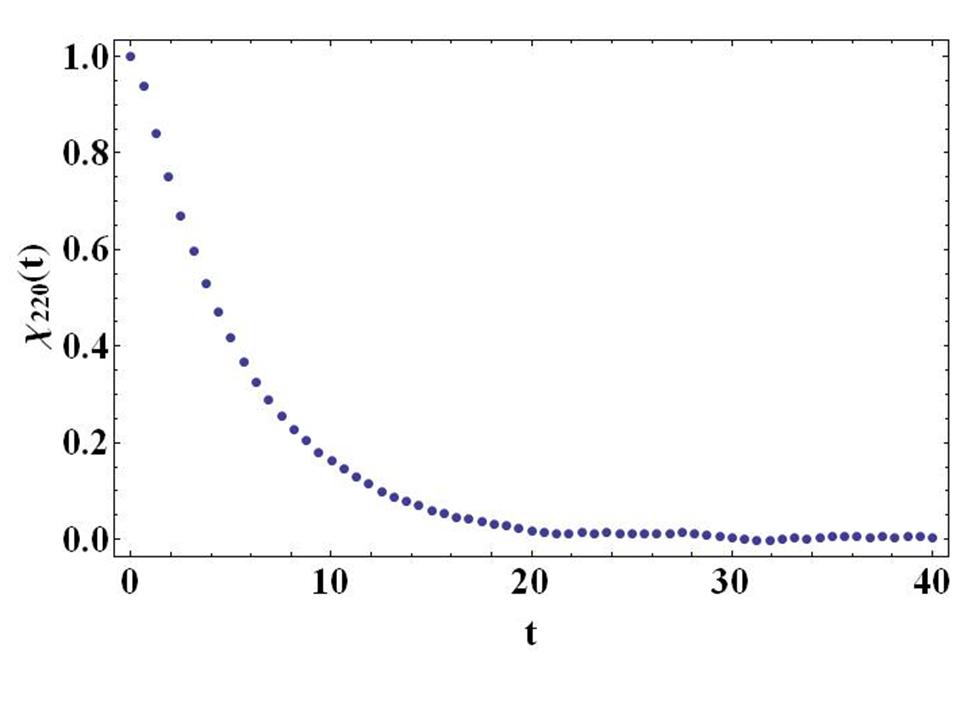
Figure 1: A typical autocorrelation, $\chi(t)$ for our model

3 Numerical Results

In this section, we review first the results of the numeric calculation of the Green-Kubo lifetimes for our model Hamiltonian. A sample of the autocorrelation as a function of time is given below (Fig. 1). It is first interesting to note that, due to the finite size of the ensemble used, the autocorrelation does not go strictly to zero for large times, so the termination of the autocorrelation is nontrivial. It would appear that, because of the finite number of degrees of freedom, the ensemble retains some memory of its initial state for arbitrarily large times. An examination of these residual ”tails” as a function of system size shows that as the system becomes large, the magnitude of the tails quickly goes to zero. For our finite systems, the $\tau$ integral was truncated after the autocorrelation dropped below 0.5 percent of the original value.

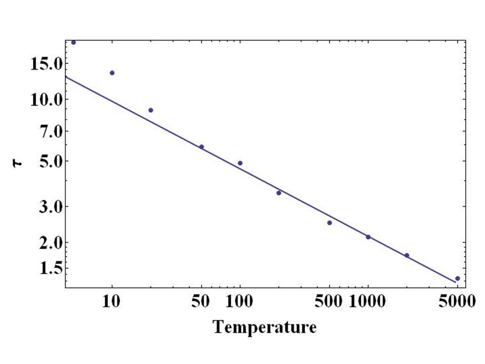
Figure 2: $\tau$ as a function of temperature in the [220] direction. The solid line represents $\tau\propto T^{-1/3}$. Note that for temperatures less than 10, the slope is steeper.

We first show how $\tau$ varies with temperature for a few wavevectors and note that the general behavior is the same for all of them (Fig. 2). As can be seen, the dependence on temperature to separate into two regions, high and low temperature being above and below about 10. For high temperatures, $\tau$ is related to temperature by a simple power law, namely

$$\tau(T)\propto T^{-\frac{1}{3}}$$ (6)

This is different from the behavior discussed by Ladd for Lennard-Jonesium, namely $\tau(T)\propto T^{-1}$. However, they expect this behavior only at low temperature. We have not determined the behavior of our model at low temperatures, because the computational times increase substantially owing to the extended lifetimes at low temperature. For the remainder of this paper, we will focus on the high temperture regime and will only note apparent deviations as we approach the transition to low temperature.

Next we examine $\tau$ along the (100), (110), and (111) directions (Fig. 3). We see here that, as expected, $\tau$ decreases with increased wavevector (as well as increased frequency), but because of the small size of the system, little more can be observed.

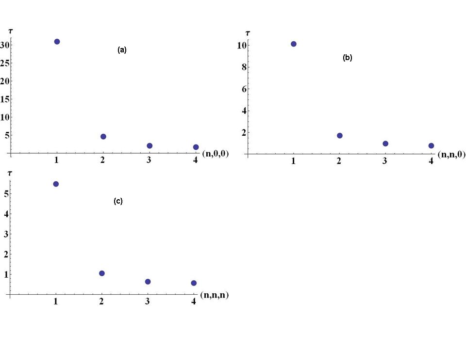
Figure 3: Tau as a function of wavevector in the (a) (1,0,0), (b) (1,1,0), and (c), (1,1,1) directions

In order to see more directly how $\tau$ is determined by the temperature and wavevector for this Hamiltonian, it is instructive to examine the behavior of the anharmonic mode frequency ($\omega_{a}(k)$). For our model Hamiltonian, we find a simple relation between the anharmonic frequency, the temperature, and the frequency in the harmonic limit ($\omega_{0}(k)$). The harmonic frequency is of the mode with wavevector $\vec{k}$ is

$$\omega_{0}(\vec{k})=\sqrt{6-2\cos{\frac{2\pi k_{x}}{l_{x}}}-2\cos{\frac{2\pi k_{y}}{l_{y}}}-2\cos{\frac{2\pi k_{z}}{l_{z}}}}$$ (7)

As can be seen in Fig. 4, the ratio between the frequency shift ($\delta\omega(\vec{k})\equiv\omega_{a}(\vec{k})-\omega_{0}(\vec{k})$) and $\omega_{0}$, depends only on temperature (that is, not on wavevector), and is well approximated by the power law

$$\frac{\delta\omega(\vec{k})}{\omega_{0}(\vec{k})}=f(T)=(T/T_{0})^{\frac{1}{3}}$$ (8)

While the exponent and possibly the simple form of the relationship is specific to our Hamiltonian, it is still an intriguing result. Based on the similarities in the exponent in Eq.  6 and  8, one reasonably suspects a relationship between the $\delta\omega$ and $\tau$. This suspicion is confirmed by examining $\tau$ as a function of $\delta\omega$ (see Fig. 5) for all wavevectors at a constant temperature, where we see again a power-law dependence.

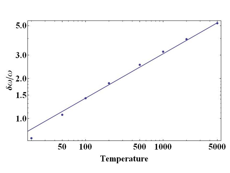
Figure 4: $\delta\omega/\omega$ as a function of temperature. This ratio is the same regardless of the wavevector examined. The solid line represents $\delta\omega/\omega\propto T^{1/3}$

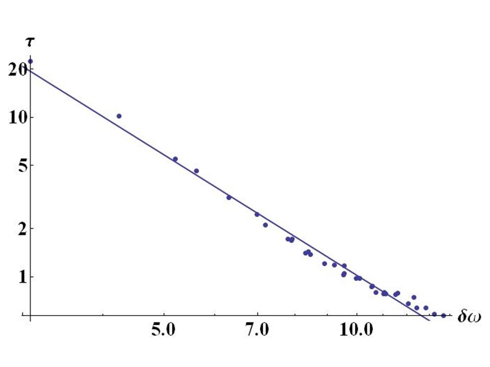
Figure 5: $\tau$ as a function of $\delta\omega$ at a temperature of 2000 for all nondegenerate wavevectors of the model used.

The implication of this relationship is that, at a fixed temperature the lifetime of a given mode depends dominantly on the anharmonic frequency. This frequency, in turn, depends on two independent factors, the harmonic frequency and the temperature.

Knowing the mode lifetimes as a function of wavevector and temperature through our numerical simulation, we can now turn to the approximate methods discussed in the companion work.

4 Approximate Methods

Because its determination does not require the use of any molecular dynamics, $\tau_{2}$ can be calculated with much less computational expense then the numerical approach considered above. Generally we have found that 200,000 MC steps is sufficient to converge $\tau_{2}$ for all temperatures and wavevectors considered here.

If we first examine the ratio $\tau_{k}/\tau_{2}$ as a function of temperature for a particular wavevector, we see that, in the high temperature regime, the ratio quickly converges to constant value (Fig. 7). While only one wavevector is shown, note that this behavior holds for all wavevectors. This is expected, due to the separable nature of the anharmonic frequency for our Hamiltonian and the dependance of $\tau$ on this frequency mentioned above. Because $\tau$ can be determined from the shift in frequency, the rest of them should display the same behavior. Because the individual wavevectors may have different shapes, the ratio may converge to different values. However, it remains true that this value is constant for a given wavevector for sufficiently high temperatures. The implication is that only $\tau_{2}$ is changing with temperature, and the $\gamma$ factors discussed above are constant.

With this notion that the shape (as opposed to the width) of $\chi(t)$ is invariant, we also test whether rescaling the elapsed time with respect to $\tau_{2}$ will cause the data to collapse onto the same curve. This is a more stringent test than the previous one as it indicates that $\chi(t)$ and not just $\tau$ can be rescaled with $\tau_{2}$. Note, in fact, that the collapse of $\chi(t)$ implies the convergence of $\tau_{k}/\tau_{2}$ seen in Fig. 6. As Fig. 7 shows, this is clearly the case in the high temperature regime. In this limit, approximating $\tau$ at the level of the second moment is sufficient to determine its behavior as a function of temperature.

Because this agreement begins to break down at lower temperatures, it may be neccesary to include higher moments as the shape of $\chi(t)$ changes from the high temperature limit. As the shape of the autocorrelation changes, some number of the $\gamma$ factors are also changing. By calculating them, and taking into account their effect on the system, a more accurate prediction of $\tau$ should be possible.

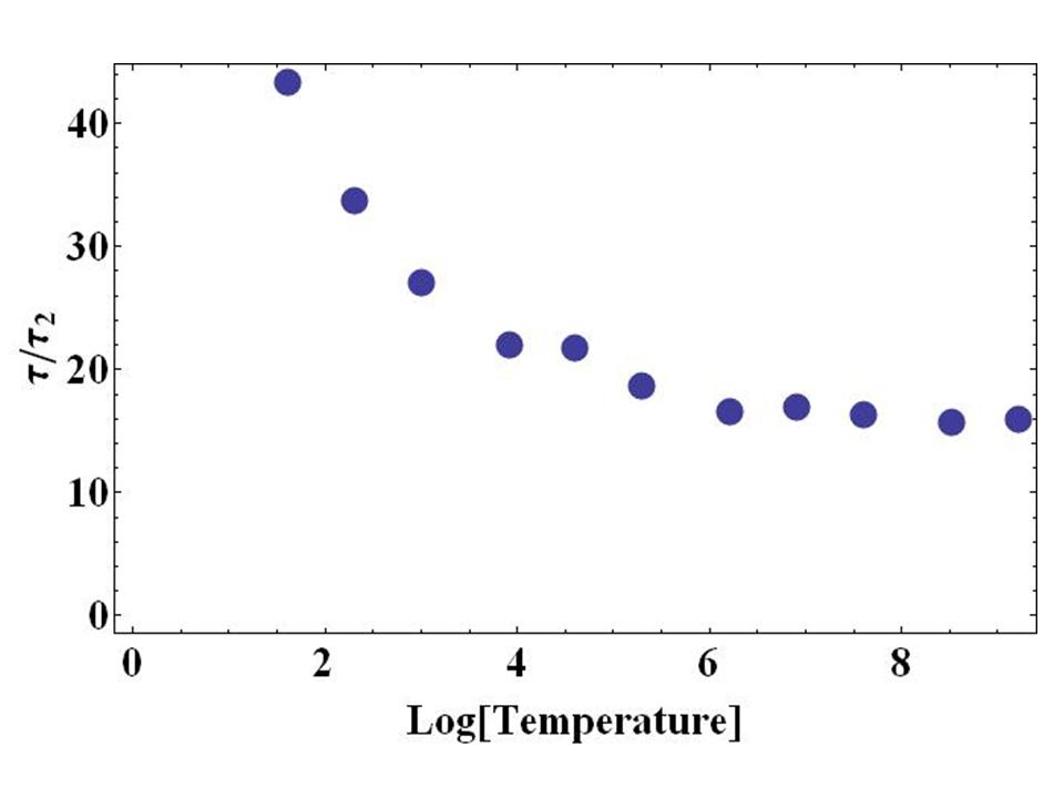
Figure 6: $\tau/\tau_{2}$ as a function of temperature. We see that $\tau_{2}$ is sufficient determine $\tau$ for high enough temperatures.

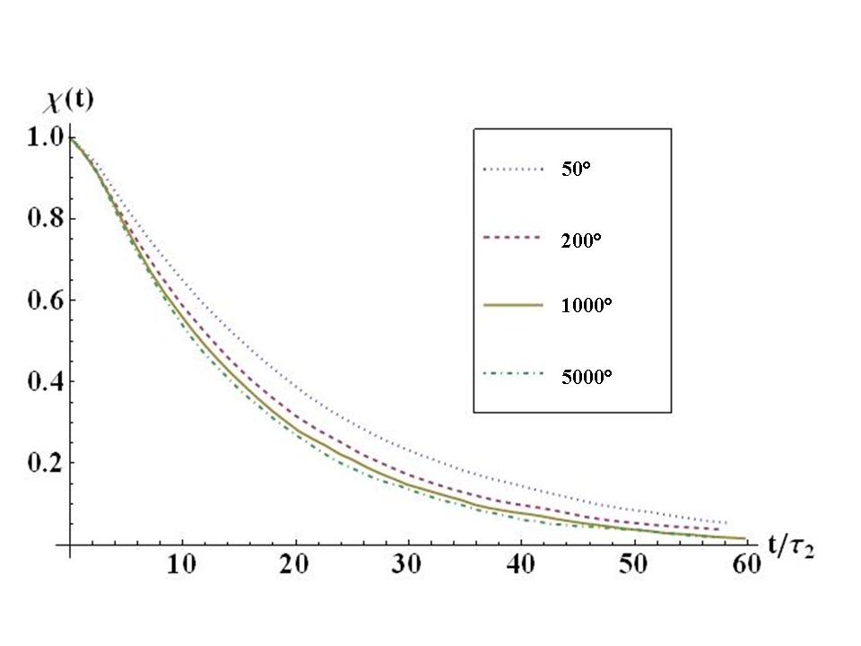
Figure 7: The data collapse of $\chi(t)$ for the [222] wavevector at several different temperatures. Because the data approach a universal curve, $\chi(t)$ and therefore $\tau$ are well-approximated, up to a constant, only by $\tau_{2}$.

5 Conclusions

By analyzing the mode lifetimes, through $\chi(t)$, in an anharmonic lattice, with a simple, quartic interaction between nearest neighbors, in three dimensions, we can draw several important conclusions. First, for this particular Hamiltonian, the lifetime of a given mode depends in a simple way on the anharmonic frequency of the mode, which in turn depends separably on the harmonic frequency and the temperature. Both of these relationships would seem to be peculiar to our model Hamiltonian, but they allow a simplified analaysis of the results. Second, seen as a function of temperature and frequency directly, $\tau$ shows a simple behavior. More generally, and most central to this work, the methodology developed in Part I is shown to be a reliable convergent method of determining the mode lifetimes with much lower computational cost than any present method of which the authors are aware. While deviations are observed for low temperatures, related to the form of the potential used, using only the first non-zero moment, $\chi(t)$ collapses effectively onto a universal curve, and $\tau$ is correctly approximated at high temperatures up to a constant to within a few percent.

While the Hamiltonian used here is a relatively simple one, which might be analyzed effectively using more direct methods, the scope of this new method should not be understated. Since calculation of lifetimes using moments requires no molecular dynamics, only averages over the ensemble, the computer time required for a calcuation is reduced dramatically, in the authors’ experience, by at least an order of magnitude or more at high temperatures, where $/tau$ is small and even more for lower temperatures as $/tau$ increases and molecular dynamics calculations must go to higher times. Furthermore, the method can be readily extended to more complicated systems. As long as $\delta n$ can be found for a member of the ensemble, $\tau_{2}$ can be derived. In addition, this formalism provides a new way of examining vibrational mode lifetimes which may provide new insights into their behavior. This improved method offers not only significant advantages in both improving the methodology of calculation but also possible insights into the mechanism of dissipation.

6 Acknowledgements

This work was partly supported by DOE (#DE-FG02-04ER-46139) and South Carolina EPSCoR.

References

- [1] R. Kubo, M. Toda, and N. Hasitsume. Nonequilibrium statistical mechanics. Springer, 1991.
- [2] D. Dickel and M. S. Daw. Improved calculation of mode lifetimes, part i: Theory. Comp. Mat. Sci., 47:698, 2009.
- [3] R. Haydock and D. Kim. Recursion solution of liouville’s equation. Comp. Phys. Comm., 87:396, 1995.
- [4] R. Haydock, C. New, and B. D. Simons. Calculation of relaxation rates from microscopic equations of motion. Phys. Rev. E, 59:5292, 1999.
- [5] R. Haydock and C. M. M. Nex. Densities of states, moments, and maximally broken time-reversal symmetry. Phys. Rev. B, 74:205121, 2006.
- [6] B. O. Koopman. Hamiltonian systems and transformations in hilbert space. Proc. Nat. Acad. Sci., 17:315, 1931.
- [7] B. O. Koopman and J. von Neumann. Dynamical systems of continuous spectra. Proc. Nat. Acad. Sci., 18:255, 1932.
- [8] R. Haydock. The recursion method. In Solid State Physics, volume 35, page 215. Academic Press, 1980.
- [9] A. J. C. Ladd, B. Moran, and W. G. Hoover. Lattice thermal conductivity: A comparison of molecular dynamics and anharmonic lattice dynamics. Phys. Rev. B, 34:5058, 1986.
- [10] G. I. Barenblatt. Scaling, self-similarity, and intermediate asymptotics. Cambridge University Press, 1996.
- [11] M. Finnis and J. Sinclair. A simple empirical n-body potential for transition metals. Phil. Mag. A, 50:45–55, 1984.
- [12] A. E. Carlsson. Beyond pair potentials in transition metals and semiconductors. In Solid State Physics, volume 43, page 1. Academic Press, 1990.